On the Computational Power of Timed
Differentiable Petri Nets
S. Haddad1, L. Recalde2, M. Silva2
1 LAMSADE-CNRS UMR 7024, University Paris-Dauphine, France
E-mail: [email protected]
2 GISED, University Zaragossa, Spain
E-mail: {lrecalde | silva}@unizar.es
Abstract. Two kinds of well studied dynamical systems are state and time discrete ones (important in Computer Science) and state and time continuous ones (heavily considered in Automatic Control). Whereas in the discrete setting, the analysis of computational power of models has led to well-known hierarchies, the situation is more confused in the con-tinuous case. A possible way to discriminate between these models is to state whether they can simulate Turing machine (or other equivalent models like counter machines). For instance, it is known that continuous systems described by ordinary differential equations (ODE) have this power. However, since the involved ODE is defined by overlapping local ODEs inside an infinite number of regions, this result has no significant application for differentiable models whose ODE is defined by an explicit representation.
In this work, we considerably strengthen this result by showing that Time Differentiable Petri Nets (TDPN) can simulate Turing machines. Indeed the ODE ruling this model is particularly simple. First its ex-pression is a linear exex-pression enlarged with the “minimum” operator. Second, it can be decomposed into a finite number of linear ODE inside polyhedra. More precisely, we present different simulations in order to fulfill opposite requirements like robustness (allowing some perturbation of the simulation) and boundedness of the simulating net system. Then we establish that the simulation of two counter machines can be per-formed by a net with a constant number of places, i.e. whose dimension of associated ODE is constant. Afterwards, by modifying the simulation, we prove that marking coverability, submarking reachability and the ex-istence of a steady-state are undecidable. Finally, we study the relations between TDPNs and time continuous Petri nets under infinite server se-mantics, a formalism with numerous results in control theory. We show that these models are equivalent and we analyse the complexity of the corresponding translations.
Keywords: Dynamic Systems, Time Differentiable Petri Nets, Expres-siveness, Simulation, Coverability, Reachability, Steady-state Analysis.
1
Introduction
Hybrid systems. Dynamic systems can be classified depending on the way time is represented. Trajectories of discrete-time systems are obtained by iterating a transition function whereas the ones of continuous-time systems are solutions of a differential equation. When a system includes both continuous and discrete transitions it is called an hybrid system. On the one hand, the expressive power of hybrid systems can be strictly greater than the one of Turing machines (see for instance [12]). On the other hand, in restricted models like timed automata [1], several problems including reachability can be checked in a relatively efficient way (i.e. they are P SP ACE-complete). The frontier between decidability and undecidability in hybrid systems is still an active research topic [8,10,4,11]. Continuous systems. A special kind of hybrid systems where the trajectories are continuous and right-differentiable functions of time have been intensively studied. They are defined by a finite number regions and associated ordinary differential equations ODEs such that inside a region r, a trajectory fulfills the equation ˙xd= fr(x) where x is the trajectory and ˙xdits right derivative. These
additional requirements are not enough to limit their expressiveness. For in-stance, the model of [2] has piecewise constant derivatives inside regions which are polyhedra and it is Turing equivalent if its space dimension is at least 3 (see also [3,5] for additional expressiveness results).
Differentiable systems. A more stringent requirement consists in describing the dynamics of the system by a single ODE ˙x = f (x) where f is continuous, thus yielding continuously differentiable trajectories. We call such models, dif-ferentiable systems. In [6], the author shows that difdif-ferentiable systems in R3
can simulate Turing machine. This result is a significant contribution to the expressiveness of differentiable systems. However this simulation is somewhat unsatisfactory:
– The ODE is obtained by extrapolation of the transition function of the Tur-ing machine over every possible configuration. Indeed such a configuration is represented as a point in the first dimension of the ODE (and also in the second one for technical reasons) and the third dimension corresponds to the time evolution.
– The explicit local ODE around every representation of a configuration is computed from this configuration and its successor by the Turing machine. So the translation is obtained from the semantics of the machine and not from its syntax.
– Thus the effective equations of the ODE are piecewise defined inside an infinite number regions which is far beyond the expressiveness of standard ODE formalisms used for the analysis of dynamical systems.
Thus the question to determine which (minimal) set of operators in an explicit expression of f is required to obtain Turing machine equivalence, is still open. Our contribution. In this work, we (partially) answer this question by showing that Time Differentiable Petri Nets can simulate Turing machines. Indeed the
ODE ruling this model is particularly simple. First its expression is a linear expression enlarged with the “minimum” operator. Second, it can be decomposed into a finite number of linear ODEs ˙x = M·x (with M a matrix) inside polyhedra. More precisely, we present different simulations in order to fulfill opposite requirements like robustness (allowing some perturbation of the simulation) and boundedness of the simulating net system. Then we establish that the simulation of two counter machines can be performed by a net with a constant number of places, i.e. whose dimension of its associated ODE is constant. Summarizing our results, TDPNs whose associated ODE is in (R≥0)6can robustly simulate Turing
machines and bounded TDPNs whose associated ODE is in [0, K]10 (for some
fixed K) can simulate Turing machines.
Afterwards, by modifying the simulation, we prove that marking coverabil-ity, submarking reachability and the existence of a steady-state are undecidable. Finally, we study the relations between TDPNs and time continuous Petri nets under infinite server semantics, a formalism with numerous results in control theory [13]. We show that these models are equivalent and we analyse the com-plexity of the corresponding translations.
Organisation of the paper. In section 2, we define TDPNs with different examples in order to give intuition about the behaviour of such systems. Then we design a first simulation of counter machines in section 3. We introduce the concept of robust simulation in section 4 and we show that the simulation is robust. Afterwards we design another (non robust) simulation by bounded nets and we transform our two simulations in order to obtain a constant number of places when simulating two counter machines. Finally, we analyse the relation between TDPNs and time continuous Petri nets in section 5. At last, we conclude and give some perspectives to this work.
2
Timed Differentiable Petri Nets
2.1 Definitions
Notations. Let f be a partial mapping then f (x) =⊥ means that f(x) is un-defined. Let M be a matrix whose domain is A× B, with A ∩ B = ∅ and a ∈ A (resp. b∈ B) then M(a) (resp. M(b)) denotes the vector corresponding to the row a (resp. the column b) of M.
Since Time Differentiable Petri Nets (TDPNS) are based on Petri nets, we recall their definition.
Definition 1 (Petri Nets). A (pure) Petri Net N = hP, T, Ci is defined by: – P , a finite set of places,
– T , a finite set of transitions with P ∩ T = ∅,
– C, the incidence matrix from P × T to N, we denote by •t (resp. t•) the
set of input places (resp. output places) of t, {p | C(p, t) < 0} (resp. {p | C(p, t) > 0}). C(t) is called the incidence of t.
Different semantics may be associated with a Petri net. In a discrete frame-work, a state m, called a marking, is a positive integer vector over the set of places (i.e. an item of NP) where an unit is called a token. The state change is triggered by transition firings. In m, the firing of a transition t with multiplicity k ∈ N>0 yielding marking m0 = m + kC(t) is only possible if m0 is positive.
Given m, kmaxthe enabling degree of t, which represents the maximal number of
simultaneous firings of t, is defined by: kmax= min(bm(p)/(−C(p, t))c | p ∈•t).
In a continuous framework, a marking m, is a positive real vector over the set of places (i.e. an item of (R≥0)P). The state change is also triggered by transition
firings. However this firing may be any “fraction” say 0 < α of the discrete firing yielding m0 = m + αC(t), possible if m0 is positive. Here, α
max the maximal
firing is defined by: αmax= min(m(p)/(−C(p, t)) | p ∈•t).
Note that in both models, the choice of the transition firing is non determin-istic. In TDPNs, this non determinism is solved by computing at any instant the instantaneous firing rate of every transition and then applying the incidence matrix in order to deduce the infinitesimal variation of the marking. The instan-taneous firing rate of transitions depends on the current marking via the speed control matrix whose meaning will be detailed in the following definitions. Definition 2 (Timed Differentiable Petri Nets). A Timed Differentiable Petri Net D = hP, T, C, Wi is defined by:
– P , a finite set of places,
– T , a finite set of transitions with P ∩ T = ∅, – C, the incidence matrix from P × T to N,
– W, the speed control matrix a partial mapping from P× T to R>0 such that:
1. ∀t ∈ T, ∃p ∈ P, W(p, t) 6=⊥
2. ∀t ∈ T, ∀p ∈ P, C(p, t) < 0 ⇒ W(p, t) 6=⊥
The first requirement about W ensures that the firing rate of any transition may be determined whereas the second one ensures that the marking remains positive since any input place of a transition will control its firing rate. Given a marking m, it remains to determine the instantaneous firing rate of a transition f (m)(t).
In TDPNs, (when defined) W(p, t) weights the impact of the marking of p on the firing rate of t. Thus we define the instantaneous firing rate similarly to the enabling degree as:
f (m)(t) = min(W(p, t)· m(p) | W(p, t) 6=⊥) We are now in position to give semantics to TDPNs.
Definition 3 (Trajectory). LetD be a TDPN, then a trajectory is a contin-uously differentiable mapping m from time (i.e. R≥0) to the set of markings
(i.e. (R≥0)P) which satisfies the following differential equation system:
˙
In fact, one can easily prove that if m(0) is positive, the requirement of positivity is a consequence of the definition of TDPNs. Moreover, one can also prove (by a reduction to the linear equation case) that given an initial marking there is always a single trajectory, i.e. the semantics of a net is well-defined and deterministic.
Equation 1 is particularly simple since it is expressed as a linear equation enlarged with the min operator. We introduce the concept of configurations: a configuration assigns to a transition, the place that will control its firing rate. Thus the number of configurations is finite. The set of markings corresponding to a configuration is a polyhedron. Inside such a polyhedron, equation 1 becomes a linear differential equation.
Definition 4 (Configuration). LetD be a TDPN, then a configuration cf of D is a mapping from T to P such that ∀t ∈ T, W(cf(t), t) 6=⊥. Let cf be a configuration, then [cf ] denotes the following polyhedron:
[cf ] ={m ∈ (R≥0)P | ∀t ∈ T, ∀p ∈ P,
W(p, t)6=⊥⇒ W(p, t) · m(p) ≥ W(cf(t), t) · m(cf(t))}
By definition, there are Qt∈T|{p | W(p, t) 6=⊥}| ≤ |P ||T | configurations.
Inside the polyhedron [cf ], the differential equation rulingD becomes linear: ∀p ∈ P, ˙m(p) =X
t∈T
C(p, t)· W(cf(t), t) · m(cf(t))
In the sequel, we use indifferently the word configuration to denote both the mapping cf and the polyhedron [cf ].
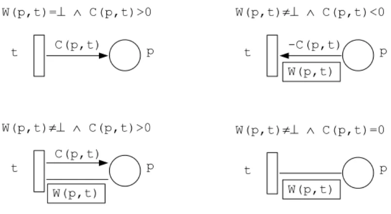
Graphical notations We extend the graphical notations of Petri net in order to take into account matrix W. A Petri net is a bipartite graph where places are represented by circles (sometimes with their initial marking inside) and transi-tions by rectangles. An arc denotes a relation between a place and a transition. Note that arcs corresponding to matrix C are oriented whereas arcs correspond-ing to matrix W are unoriented. We describe below the four possible patterns illustrated in figure 1.
– W(p, t) =⊥ ∧ C(p, t) > 0, place p receives tokens from t and does not control its firing rate. There is an oriented arc from t to p labelled by C(p, t) – W(p, t) 6=⊥ ∧ C(p, t) < 0, place p provides tokens to t. So it must control
its firing rate. The unoriented arc between p and t is redundant, so we will not draw it and represent only an oriented arc from p to t both labelled by−C(p, t) and W(p, t). In order to distinguish between these two labels, W(p, t) will always be drawn inside a box.
– W(p, t) 6=⊥ ∧ C(p, t) > 0, place p receives tokens from t and controls its firing rate. There is both an oriented arc from t to p and an unoriented arc between p and t with their corresponding labels.
– W(p, t)6=⊥ ∧ C(p, t) = 0, place p controls the firing rate of t and t does not modify the marking of p. There is an unoriented arc between p and t.
Fig. 1.Graphical notations
We omit labels C(p, t),−C(p, t) and W(p, t) when they are equal to 1.
The first two patterns occur more often in the modelling of realistic systems than the two other ones. In section 5, we will show that the two last patterns may be simulated (with some increasing of the net size).
2.2 Examples
In order to simplify the notations, when writing the differential equations, we use p as a notation for m(p) (the trajectory projected on p).
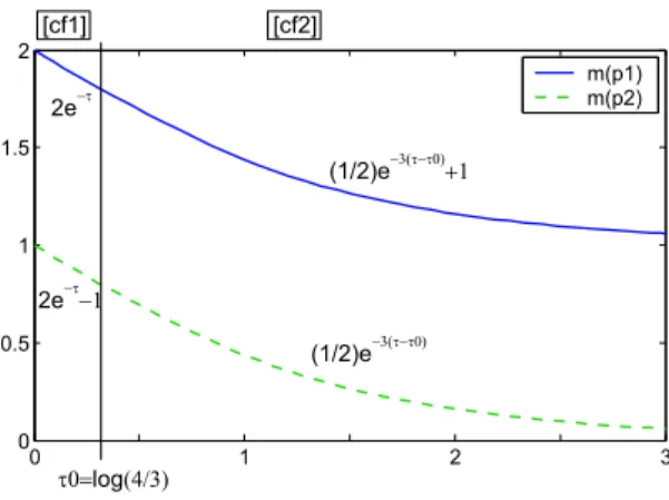
Fig. 2.A marked net switching once
A configuration switch. The net of figure 2 illustrates the main concepts of TDPNs. The firing rate of t is given by f (m)(t) = min(m1(p), 3m2(p)). Thus
equation 1 becomes:
There are two configurations [cf1] = {m | m(p1) ≤ 3m(p2)} and [cf2] =
{m | m(p1 ≥ 3m(p2)}. Inside [cf1], equation 1 becomes ˙p1 = ˙p2 = −p1 and
inside [cf2], equation 1 becomes ˙p1= ˙p2=−3p2.
The behaviour of this net can be straightforwardly analysed. It starts in [cf1] where it stays until it reaches marking m = (3/2, 1/2). Then it switches to
configuration [cf2] where it definitely stays and ultimately reaches the
steady-state marking (0, 0). This behaviour is illustrated in figure 3.
0 1 2 3 0 0.5 1 1.5 2 m(p1) m(p2) [cf1] [cf2] 2e-t 2e-t-1 (1/2)e-3(t-t0)+1 (1/2)e-3(t-t0) t0=log(4/3)
Fig. 3.The behaviour of net of figure 2
Infinitely switching. Let us suppose that a marked TDPN has a steady-state. This steady-state belongs to (at least) one configuration and fulfills the equation for steady-states (i.e. C· f(m) = 0) which is a linear equation inside a configuration. Thus the identification of possible steady-states is reduced to the identification of such states for every configuration.
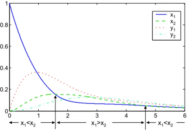
One may wonder whether the asymptotical behaviour of a net approaching a steady-state can be reduced to the corresponding behaviour for every configu-ration. This would be the case if a marked net leading to a steady-state switches between configurations only a finite number of times as does the the net of pe-vious examples. However as the analysis of the net of figure 4 will show, a net may infinitely switch between configurations while reaching a steady-state.
The ordinary differential equation corresponding to this net is:
˙x1= f (t4)− f(t1)− f(t) = y2− x1− min(x1, x2)
˙x2= f (t2)− f(t3)− f(t) = y1− x2− min(x1, x2)
˙y1= f (t1)− f(t2) = x1− y1
Fig. 4.A net infinitely switching
The two configurations of this net are [cf1] = {m | m(x1) ≥ m(x2)} and
[cf2] ={m | m(x1)≤ m(x2)}. Its evolution can be observed in Fig. 5.
0 1 2 3 4 5 6 0 0.2 0.4 0.6 0.8 1 x1 x2 y1 y2 x >x1 2 x <x1 2 x <x1 2
Fig. 5.Evolution of the system described by the net of fig. 4
Observation. The net of figure 4 reaches a steady state while infinitely switching between configurations.
Proof. Let us write some behavioural equations related to this net. We note δx= m(x1)− m(x2) and δy= m(y1)− m(y2). Then:
˙δx=−δx− δy
˙δy= δx− δy
Taking into account the initial conditions, these equations yield to: δx= e−τcos(τ )
δy= e−τsin(τ )
Thus the net infinitely switches between configuration m(x1) ≥ m(x2) and
m(x1)≤ m(x2).
It remains to show it (asymptotically) reaches a steady-state. Let us note s = m(x1) + m(x2) + m(y1) + m(y2).
One has ˙s =−2 inf(x1, x2). Thus s is decreasing, let us note l its limit.
We show that l = 0. Assume that l > 0.
Since limτ →∞δx(τ ) = 0, there is a n0 such that:
∀n ≥ n0,|m(x1)((2n + 1)π)− m(x2)((2n + 1)π)| ≤ l/4.
Since m(y1)((2n + 1)π) = m(y2)((2n + 1)π),
we conclude that:
∀n ≥ n0, either m(y1)((2n + 1)π) = m(y2)((2n + 1)π)≥ l/4
or min(m(x1)((2n + 1)π), m(x2)((2n + 1)π))≥ l/8.
We note τ0= (2n + 1)π and τ any value greater or equal than τ0.
Case m(y1)(τ0) = m(y2)(τ0)≥ l/4
The following inequation holds: ˙m(yi)≥ −m(yi).
Thus m(yi)(τ )≥ (l/4)e−(τ −τ0)and ˙m(xi)≥ (l/4)e−(τ −τ0)− 2m(xi).
Consequently, m(xi)(τ )≥ (m(xi)(τ0) + (l/4)(eτ −τ0− 1))e−2(τ −τ0)
≥ (l/4)(eτ −τ0 − 1)e−2(τ −τ0). Finally, s(τ0)− s(τ0+ 2π)≥ R2π 0 (l/2)(e v − 1)e−2vdv.
Call this last value d1.
Case min(m(x1)(τ0), m(x2)(τ0))≥ l/8
The following inequation holds: ˙m(xi)≥ −2m(xi).
Consequently, m(xi)(τ )≥ (l/8)e−2(τ −τ0)
Finally, s(τ0)− s(τ0+ 2π)≥R02π(l/4)e−2vdv.
Call this last value d2.
Summarizing, one obtains s((2n + 1)π) ≤ s((2n0+ 1)π)− (n − n0)min(d1, d2)
in contradiction with positivity of s.
Periodic behaviour. The last example shows that the asymptotic behaviour of a net may strongly depend on the configurations it reaches.
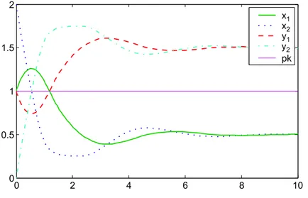
Fig. 6.A periodic TDPN
The ordinary differential equation corresponding to the net of Figure 6 is (note that place pk holds a constant number of tokens):
˙x1= f (t2)− f(t4) = min{ω · x2, 2aω· y1} − min{aω · x1, ω}
˙x2= f (t1)− f(t3) = min{aω · y2, ω} − min{2aω · x2, ω· x1}
˙y1= f (t4)− f(t2) = min{aω · x1, ω} − min{ω · x2, 2aω· y1}
˙y2= f (t3)− f(t1) = min{2aω · x2, ω· x1} − min{aω · y2, ω}
However, it can be observed that y1+ x1 and y2+ x2 are constant. Hence
the system (with the initial condition described by the marking in the figure) is equivalent to:
˙x1= min{ω · x2, 2aω· y1} − min{aω · x1, ω· a}
˙x2= min{aω · y2, ω· a} − min{2aω · x2, ω· x1}
y1= 2a− x1
y2= 2a− x2
This corresponds in fact to a set of sixteen configurations. Let us solve the differential system with 1 ≤ a ≤ b ≤ 2a − 1. The linear system that applies
initially is:
˙x1= ω· x2− ω · a
˙x2= ω· a − ω · x1
y1= 2a− x1
y2= 2a− x2
In figure 6, we have represented the “inactive” items of matrix W in a shad-owed box. In the sequel, we use this convention when it will be relevant. The solution of this system is:
x1(τ ) = a + (b− a) sin(ω · τ)
x2(τ ) = a + (b− a) cos(ω · τ)
y1(τ ) = a− (b − a) sin(ω · τ)
y2(τ ) = a− (b − a) cos(ω · τ)
This trajectory stays infinitely in the initial configuration and consequently it is the behaviour of the net. However for other initial conditions like a = 1, b = 2, configuration switches happen before a steady state is ultimately reached, as can be observed in figure 7. 0 2 4 6 8 10 0 0.5 1 1.5 2 x2 x1 y1 y2 pk
Fig. 7.Evolution of the system described by the net of Fig. 6 with a = 1, b = 2
Remark. This example illustrates the fact that the dimension of the ODE may be strictly smaller than the number of places. Indeed, the existence of a linear
invariant suchPp∈Pm(p) = cst decreases by one unit the number of dimensions.
Otherwise stated, the dimension of the ODE is not |P | but rank(C). In the example,|P | = 5 and rank(C) = 2.
3
A first simulation
3.1 Preliminaries
Counter machines. We will simulate counter machines which are equivalent to Turing machines. A counter machine has positive integer counters, (note that two counters are enough for the equivalence [9]). Its behaviour is described by a set of instructions. An instruction I may be one of the following kind with an obvious meaning (cptu is a counter):
– I: goto I’;
– I: increment(cptu); goto I’;
– I: if cptu= 0 then goto I’ else decrement(cptu); goto I";
– I: STOP;
In order to simplify the simulation, we split the test instruction as follows: – I: if cptu= 0 then goto I’ else goto Inew;
– Inew: decrement(cptu); goto I";
Furthermore, w.l.o.g. we assume that the (possible) successor(s) of an in-struction is (are) always different from it.
Dynamical systems and simulation. The (deterministic) dynamical systems (X,T , f) we consider are defined by a state space X, a time space T (T is either Nor R≥0) and a transition function f from X× T to X fulfilling:
∀x ∈ X, ∀τ1, τ2∈ T , f(x, 0) = x ∧ f(x, τ1+ τ2) = f (f (x, τ1), τ2)
In a discrete system X ⊆ Nd for some d andT = N whereas in a continous
system X⊆ (R≥0)d for some d andT = R≥0.
The simulation of a discrete system by a continuous one involves a mapping from the set of states of the discrete system to the powerset of states of the continuous systems and an observation epoch. The requirements of the next definition ensure that, starting from some state in the image of an initial state of the discrete system and observing the state reached after some multiple n of the epoch, one can recover the state of the discrete system that would have been reached after n steps.
Definition 5. A continuous dynamical system (Y, R≥0, g) simulates a discrete
dynamical system (X, N, f ) if there is a mapping φ from X to 2Y and τ
0∈ R>0
such that:
– ∀x 6= x0∈ X, φ(x) ∩ φ(x0) =∅
3.2 Basic principles of the simulation
Transition pairs. In a TDPN, when a transition begins to fire, it will never stop. Thus we generally use transition pairs in order to temporarily either move tokens from one place to another one, or produce/consume tokens in a place.
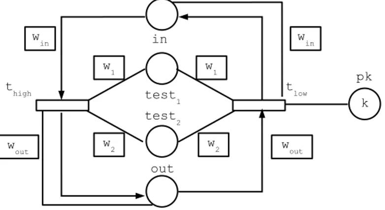
Fig. 8.A transition pair
Let us examine transitions thighand tlow of figure 8. Their incidence is
oppo-site. So if their firing rate is equal no marking change will occur. Let us examine W, all the items of W(thigh) and W(tlow) are equal except W(pk, tlow) = k
and W(pk, thigh) =⊥. Thus, if any other place controls the firing rate of tlow it
will be equal to the one of thigh. Place pk is a constant place meaning that its
marking will always be k. So we conclude that:
– if winm(in) > k∧ woutm(out) > k∧ w1m(test1) > k∧ w2m(test2) > k then
this pair transfers some amount of tokens from in to out, – otherwise, there will be no marking change.
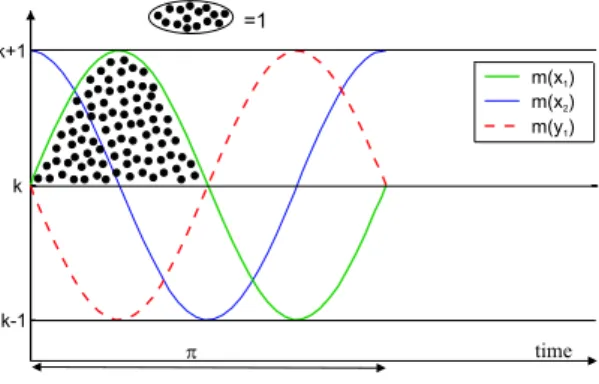
The clock subnet. The net that we build consists in two subnets: an instance of the subnet of figure 6 that we will call in the sequel the clock subnet and another subnet depending on the counter machine. We call this latter subnet, the operating subnet.
The clock subnet has k as average value, 1 as amplitude and π as period (i.e. ω = 2). We recall the behavioural equations of the place markings that will be used by the operating subnet:
m(x1)(τ ) = k + sin(2τ ), m(y1)(τ ) = k− sin(2τ)
Figure 9 represents the evolution of markings for x1, y1and x2(the marking
of place y2 is symmetrical to x2 w.r.t. the axis m = k). Note that the mottled
k-1 k k+1 m(x )2 m(x )1 m(y )1 p time =1
Fig. 9.The behaviour of the clock subnet
The marking changes of the operating subnet will be ruled by the places x1
and y1. An execution cycle of the net will last π. The first part of the cycle (i.e.
[hπ, hπ + π/2] for some h∈ N) corresponds to m(x1)≥ k and the second part
of the cycle (i.e. [hπ + π/2, (h + 1)π]) corresponds to m(y1)≥ k.
So, the period of observation τ0is equal to π.
At last, note that place pk occurring in the transition pairs is the constant place of the clock subnet.
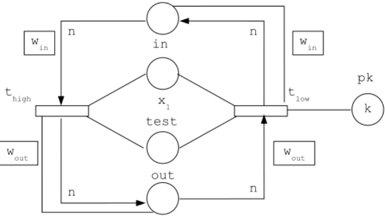
Specialisation of the transition pairs pattern. Using places x1and y1, we
specialise transition pairs as illustrated in figure 10. In this subnet, one of the test place is x1and the control weights of the two test places (x1and test) are 1.
First due to the periodical behaviour of m(x1), we know that no tokens transfer
will occur during the second part of the cycle. Let us examine the different cases during a time interval [hπ, hπ + π/2]. We assume that within this interval m(test), m(in) and m(out) are not modified by the other transitions.
– If m(test)(hπ)≤ k then there will be no transfer of tokens.
– If m(test)(hπ)≥ k+1∧win(m(in)(hπ)−n) ≥ k+1∧woutm(out)(hπ)≥ k+1
then thigh will be controlled by x1 and tlow will be controlled by pk. Hence
(see the integral of figure 9) exactly n tokens will be transfered from in to out.
– In the other cases, some amount of tokens in [0, n] will be transfered from in to out.
From a simulation point of view, one wants to avoid the last case. Thus in some marking m, we say that a place is active if m(p)≥ k + 1 and inactive if m(p)≤ k. For the same reason, when possible, we choose winand wout enough
Fig. 10.A specialised transition pair
3.3 The operating subnet
Places of the operating subnet and the simulation mapping. Let us suppose that the program with counters has l instructions {I1, . . . , Il} and
two counters{cpt1, cpt2}. The operating subnet will have the following places:
S
1≤i≤l{pci, pni} ∪ {c1, c2}.
We now define the simulation mapping φ, Assume that, in a state s of the counter machine, Iiis the next instruction and the value of the counter cptuis
vu.
Then a marking m∈ φ(s) iff:
– The submarking corresponding to the clock subnet is its initial marking (note that this is independent from the state of the machine).
– m(pni) = k + 2 and m(pci)∈ [k + 2, k + 11/4], note that these places are
active. – ∀1 ≤ i0
6= i ≤ l, m(pni0) = k−1 and ∀1 ≤ i0 6= i ≤ l, m(pci0)∈ [k−1, k−1/4],
note that these places are inactive.
– m(c1) = k− 1 + 3v1, m(c2) = k− 1 + 3v2, thus we choose a affine
trans-formation of the counter values. Note that if such a value is 0 then the corresponding place is inactive whereas if it is non null, the place is active. Thus the difference between the marking of an active pniand an inactive pnj
is 3 as is the difference between the marking interval for an active pci and an
inactive pcj. We will progressively explain the choices relative to this mapping,
during the presentation of the operating subnet transitions.
Finally note that k will be chosen enough large to fulfill additional constraints when needed.
Principle of the instruction simulation. The simulation of an instruction Iiwill take exactly the time of the cycle of the clock subnet and is decomposed
in two parts (m(x1)≥ k followed by m(y1)≥ k).
The first stage is triggered by m(pci) ≥ k + 1 and performs the following
tasks:
– decrementing pni(by 3) while incrementing pnj (by 3) where Ijis the next
instruction. If Iiis a conditional jump, this involves to find the appropriate
j. The marking of pni will vary from k + 2 to k− 1 and vice versa,
– updating the counters depending on the instruction.
The second stage is triggered by m(pnj)≥ k + 1 and performs the following
tasks:
– incrementing pcj (by 3) and decrementing pci by a variable value in such
a way that their marking still belong to the intervals associated with the simulation mapping,
– by a side effect, possibly decrementing some inactive pci0but not below k−1.
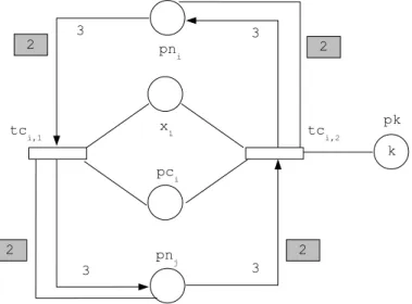
First stage: simulation of an unconditional jump. This part of the simula-tion applies to both an uncondisimula-tional jump, an incrementasimula-tion and a decremen-tation. We explain in the next paragraph how the counter updates are performed. For this kind of instructions, the next instruction say Ijis a priori known.
This subnet consists in a transition pair which transfers, during the first part of the cycle (due to the place x1), 3 tokens from pni to pnj iff pci is active (i.e.
if the simulated instruction is Ii).
Note that the value W(pni, tci,1) = W(pni, tci,2) = W(pnj, tci,1)
= W(pnj, tci,2) = 2 ensures that places pni and pnj will not control these
transitions (since 2(k− 1) ≥ k + 2 for k enough large).
First stage: counter updates. The update of counters does not raise any par-ticular problem as illustrated in the figure 12. We connect place cuto the previous
transition pair depending whether it is an incrementation or a decrementation. During the first part of the cycle, the place cureceives or looses the same quantity
of tokens as the one received by pnj, i.e. 3. Again W(cu, tci,1) = W(cu, tci,2) = 2
ensures that cuwill not determine the firing rate of the transitions.
Fig. 12.Counter updates
First stage: simulation of a conditional jump. The first stage for simulat-ing the instruction Ii: if cptu= 0 then goto Ijelse goto Ij0; is illustrated in
figure 13.
It consists in two transition pairs. Pair tci,1, tci,2mimics the first stage of an
unconditional jump from Ii to Ij. It will transfer during the first part of the
cycle 3 tokens from pnito pnj. Pair tci,3, tci,4is triggered if both pciand cu are
active (i.e. the counter cptuis non null). If it is the case it will transfer 3 tokens
from pnj to pnj0. Thus:
– If m(cu) = k− 1 then only the first pair is triggered and 3 tokens will be
Fig. 13.The first stage of a conditional jump
– otherwise m(cu) ≥ k + 2, the two pairs are simultaneously triggered and
3 tokens will be transfered from pni to pnj and from pnj to pnj0. So the
marking of pni looses 3 tokens, pnj is unchanged and pnj0 receives 3 tokens
as desired.
Fig. 14.The second stage: incrementing pcj
The second stage. The second stage consists in incrementing pcj and
decre-menting pci. The first operation does not raise any particular difficulty and is
illustrated figure 14.
Pair tnj,1, tnj,2is triggered by place pnj which has become active during the
first stage (note that the stage is controlled by y1). In fact, this pair is only
The decrementation of pci is the difficult part of the simulation. Indeed,
different instructions may jump to Ij. So the transition pair of figure 15 is
triggered both by pnj and pci. Note that we create such transitions for every
pair Ii, Ij of instructions such that Ij possibly follows Ii. Let us explain the
weight W(pci) = k/(k− 1): with such a weight the pair is only triggered if
m(pci)≥ k − 1 and then if Ijis reached by another instruction than Ii, m(pci)
could decrease but not below k− 1 as it is required for the simulation.
Fig. 15.The second stage: decrementing pci
However this additional control has a drawback since if m(pci) = k + 2 at the
beginning of the second part of the cycle, this place will control the firing of tni,j,1
during this part as can been observed in figure 16. Thus pciwill loose less than 3
tokens. In this figure, we have drawn three curves related to (k/(k− 1))m(pci):
– the first one which finishes as a dotted line would be (k/(k − 1))m(pci)
with m(pci) = k + 2 at the beginning of the stage, if m(y1) had controlled
the firing rate during the whole stage, and then 3 tokens would have been transfered;
– the second one which is identical to the first one at the beginning is the real (k/(k− 1))m(pci) with m(pci) = k + 2 at the beginning of the stage, and
less 3 tokens have been transfered;
– the third one is (k/(k− 1))m(pci) with m(pci) = k + 11/4 at the beginning
of the stage. We claim that this curve does not meet m(y1) and then exactly
3 tokens have been transfered.
Proof of the claim. In order to prove it we write the equation of m(pci)
when the firing rate is always controlled by m(y1) and we verify that (k/(k−
Fig. 16.Which place does control tni,j,1?
We choose the beginning of the second part as the origin of time and study functions during the interval [0, π/2].
– (k/(k− 1))m(pci)(τ ) = (k/(k− 1))(k + 5/4 + (3/2)cos(2τ)
≥ (1 + 1/k)(k + 5/4 + (3/2)cos(2τ)
= (k + 9/4 + (3/2)cos(2τ ) + (1/k)(5/4 + (3/2)cos(2τ )) ≥ k + (3 +√2)/2 + (3/2)cos(2τ ) for k enough large. Let us note ϕ(τ ) = k + (3 +√2)/2 + (3/2)cos(2τ ), then ϕ(3π/8) = k + (3 +√2)/2− 3√2/4≥ k + 1 and ϕ(π/2) = k + (3 +√2)/2− 3/2 = k +√2/2. Since ϕ(τ ) is decreasing, we conclude that: ∀0 ≤ τ ≤ 3π/8, ϕ(τ) ≥ k + 1
and∀3π/8 ≤ τ ≤ π/2, ϕ(τ) ≥ k +√2/2
– m(y1)(τ ) = k + sin(2τ ), thus∀0 ≤ τ ≤ π/2, m(y1)(τ )≤ k + 1.
Furthermore, m(y1)(3π/8) = k +
√ 2/2.
Since m(y1) is decreasing in [3π/8, π/2], we conclude that:
∀3π/8 ≤ τ ≤ π/2, m(y1)(τ )≤ k +√2/2
So the claim is established.
We illustrate in figure 17 the evolution of m(pci) at observation epochs. Note
that the dotted lines do not represent the evolution of marking but just bind the corresponding values between observation epochs.
The following theorem is a direct consequence of the correctness of our con-struction.
Theorem 1. Given a counter machineM, one can build a TCPN D whose size is linear w.r.t. the machine such thatD simulates M.
Fig. 17.Evolution of m(pci,j,1) at observation epochs
4
Refining the simulation
4.1 Robust simulation
In order to introduce robust simulation, we refine the notion of simulation. First, we consider a two-level dynamical system (Y = Y1× Y2, R≥0, g) such that g is
defined by g1from Y1×R≥0to Y1and by g2from Y×R≥0to Y2as: g((y1, y2), τ ) =
(g1(y1, τ ), g2((y1, y2), τ ). In words, the behaviour of the first component depends
only on its local state.
Definition 6. A two-level continuous dynamical system (Y, R≥0, g) consistently
simulates a discrete dynamical system (X, N, f ) if there is y0∈ Y1, a mapping φ
from X to 2Y2 and τ 0∈ R>0 such that: – ∀x 6= x0 ∈ X, φ(x) ∩ φ(x0) = ∅, – g1(y0, τ0) = y0,
– ∀x ∈ X, ∀y ∈ φ(x), g2((y0, y), τ0)∈ φ(f(x, 1)).
The critical remark here is that the first part of component is a “fixed” part of the system since its whole trajectory does not depend on the input of the simulated system. The robustness of the simulation is related to pertubations of the function φ and to the time of observations. In the following definition, dist is the distance related to norm| |∞(but the definition is essentially independent
from the choice of the norm).
Definition 7. A simulation (by a two-level system) is robust iff there exists δ, ²∈ R>0 such that:
– ∀x 6= x0∈ X, dist(φ(x), φ(x0)) > 2²
– ∀x ∈ X, ∀y2∈ Y2,∀n ∈ N, ∀τ ∈ R≥0,
max(dist(y2, φ(x)), dist(τ, nτ0))≤ δ ⇒ dist(g2((y0, y2), τ ), φ(f (y, n)))≤ ²
Thus, if the simulation is robust, starting with an initial no more pertubated than δ and delaying or anticipating the observation of the system by no more than δ, the state of the simulated system can be recovered.
Theorem 2. Given a counter machineM, one can build a TDPN D whose size is linear w.r.t. the machine such thatD robustly simulates M.
Proof. We prove that our simulation is robust. Note that this simulation is a two-level simulation with places of kind pci, pni, cu corresponding to the simulation
mapping. We choose δ = min(1/4, 1/24(k + 1)|T |) and ² = 1/2.
First note that due to our modelling, two markings simulating different con-figurations x and x0 of the machine have at least one place where they differ by
at least 3/2(> 1) tokens. So ² fulfills the first requirement of robustness. The behaviour of the net is driven by firing rate differences between transition pairs. So this behaviour depends on the “activity” of places pci, pni, cu in the
following way: an inactive place may have any marking in [k− 5/4, k] and an active behaviour may have a marking in in [k +7/4, k +3]. Indeed, the important point is that an inactive place has a marking m≤ k and an active place has a marking m≥ k + 1.
Thus a initial perturbation in [0, 1/4], will yield a perturbation at observation epochs which may vary but will be always in [0, 1/4].
Since the behaviour of the net is ruled by a differential equation, let us bound| ˙m|. First note that ∀p, t, |C(p, t)| ≤ 3. Then a simple examination of the transitions of the net shows that∀t, f(m)(t) ≤ 2(k + 1). Thus | ˙m| ≤ 6(k + 1)|T |. Thus a perturbation of the observation epoch with a value≤ 1/24(k + 1)|T | leads to a pertubation of the marking with a value≤ 1/4.
Summing the two perturbations yields the result.
4.2 Simulation with a bounded TDPN
In this paragraph, we modify our simulation in order to obtain a bounded net. Note that bounded and robust simulations of an infinite-state system are incom-patible for obvious reasons. Our current net is unbounded due to the way we model the counters. So we change their management.
First we will build a new lazy machineM0from the original oneM. We
multi-ply by 4 the number of intructions, i.e. we create three instructions Ai: goto Bi;,
Bi: goto Ci; and Ai: goto Ii; per instruction Ii. Then we modify every label
in the original instructions by substituting Ai to Ii.M and M0 are equivalent
from a simulation point of view since they perform the same computation except that four instructions ofM0 do what does a single of instruction of
M. We then duplicate the operating subnet (D0(1)and
D0(2)) to simulate
M via M0. The only difference between the subnets is that
D0(1)simulates I
iofM by
This yields the scheduling given in figure 18. We will also use the superscripts
(1) and(2) to distinguish between places of the two subnets.
Fig. 18.Interleaving two simulations
In each subnet, we create a place d(s)u (s = 1, 2) in addition to c(s)u , to model
the counter cptu. Then we change our counter updates in such a way that when
a counter cptu is equal to v then m(c (s) u ) = (k + 2)− 2(1/2)v and m(d(s)u ) = (k− 1) + 2(1/2)v. Hence if cptu= 0 then m(c (s) u ) = k and if cptu≥ 1 then m(c (s) u )≥ k + 1 as
required for the correctness of the simulation of the conditional jump.
It remains to describe the handling of incrementations and decrementations. Note that the main difficulty is that the decrement (or increment) depends on the current value of the simulated counter. If cptu= v and we increment the
counter, then we must produce (resp. consume) (1/2)v tokens in c(s)
u (resp. in
d(s)u ). If cptu= v and we decrement the counter, then we must consume (resp.
produce) (1/2)v+1 tokens in c(s)u (resp. in d(s)u ).
Let us observe the evolution of marking pni in the first simulation (see
fig-ure 19) when one simulates the execution of instruction Ii. In the first part of
a cycle it raises from k− 1 to k + 2, then holds this value during the second part and decreases in the first part of the next cycle to k. The increasing and the decreasing are not linear but they are symmetrical. Thus the mottled area of figure 19 is proportional to the difference between cu and k + 2 (equal to the
difference between du and k− 1). We emphasize the fact that neither the upper
part of this area nor its lower part are proportional to the difference.
The subnets of figure 20 and figure 21 exploit this feature to simulate an incrementation of the counter. Ii is an incrementation of the counter cptu. Let
us detail the behaviour of the former subnet.
This subnet has two transition pairs inci,1, inci,2and inci,3, inci,4. The firing
Fig. 19.A way to obtain a “proportional” increment
speed control equal to 1, places c(1)u and c(1)u do not determine this rate). The
rate of inci,2 is (1/(4π))m(pn(1)i ). Thus they have different speed as long as
m(pn(1)i ) > m(c (2)
u ). So their effect corresponds to the upper part of the mottled
area of figure 19.
The rate of inci,3 is (1/(4π))min(m(d(2)u ), m(pn(1)i )). The rate of inci,4 is
(k− 1)/(4π). So their effect corresponds to the lower part of the mottled area of figure 19.
The scaling factor 1/4π ensures that 1/2(m(d(2)u )− (k − 1)) have been
trans-fered from m(d(1)u ) to m(c(1)u ).
The net of figure 21 behaves similarly except that since m(c(1)u ) and m(d(1)u )
have their new value the scaling factor must be doubled in order to transfer the same amount of tokens from m(d(2)u ) to m(c(2)u ).
The decrementation simulation follows the same pattern except that the scal-ing factor of the first stage is doubled w.r.t. the first stage of the incrementation whereas the scaling factor of the second stage is divided by two w.r.t. the second stage of the incrementation.
It remains to show that the places ofD0(2) modelling the counter cpt u are
not modified during the simulation of the IiinD0(1)and vice versa. Looking at
figure 22 we see that this is the case as the instruction simulations are translated and surrounded by “no-op” instructions which do not modify the counters.
The correctness of this simulation yields the following theorem.
Theorem 3. Given a counter machine M, one can build a bounded TDPN D whose size is linear w.r.t. the machine such that D simulates M.
Note that, the speed control matrix of this net has non rational items con-trary to the net of the first simulation. They belong to the field Q[π]. It is an
Fig. 20.Incrementing a counter (first stage)
Fig. 22.Non interference between the counter updates
open question whether one can build a simulating bounded net and a simulation mapping with only rational numbers.
4.3 Simulation with a constant number of places
In this paragraph, we show that we can transform our previous simulations such that the number of places is independent from the two counter machine (with l > 1 instructions) which is simulated. We develop the case of a robust simulation, the adaptation to a bounded simulation is similar to the one of the previous section.
In order to build such a simulation we change the way, we manage the sim-ulation of the program counter. Instead of places pci, pni, we will use 4 places:
– pc, qc corresponding to the set of places{pci},
– pn, qn corresponding to the set of places{pni},
We do not change places associated with counters. We choose k≥ 6l2.
We now define the simulation mapping φ, Assume that, in a state s of the counter machine, Iiis the next instruction and the value of the counter cptuis
vu.
Then a marking m∈ φ(s) iff:
– The submarking corresponding to the clock subnet is its initial marking. – m(pn) = i, m(qn) = l + 1− i,
m(pc)∈ [i − l/k, i + l/k] and m(qc) ∈ [l + 1 − i − l/k, l + 1 − i + l/k] else if i = 1 m(pc)∈ [1, 1 + l/k] and m(qc) ∈ [l − l/k, l] else if i = l m(pc)∈ [l − l/k, l] and m(qc) ∈ [1, 1 + l/k] – m(c1) = k− 1 + 3v1, m(c2) = k− 1 + 3v2.
The principle of the simulation is the same as before: a cycle is divided in two parts. We detail the differences between the new simulation and the original one.
First stage: simulation of an unconditional jump The subnet we build depends on the relative values of i (the index of the current instruction) and j (the index of the next instruction). Here, we assume that i < j, the other case is similar. The transition pair of figure 23 is both triggered by pc and qc.
– Assume that the current instruction is Ii0 with i0 6= i. If i0 < i then pc
disables the transition pair whereas if i0 > i then qc disables the transition
pair. We explain the first case. m(pc)≤ i0+ l/k
≤ i − 1 + l/k; thus ((k + 3l)/i)m(pc)≤ ((k + 3l)/i)(i − 1 + l/k) ≤ k − 1 (due to our hypothesis on k).
– Assume that the current instruction is Ii.
Then both ((k + 3l)/i)m(pc)≥ ((k + 3l)/i)(i − l/k) ≥ k + 2
and ((k +3l)/(l +1−i))m(qc) ≥ ((k +3l)/(l+1−i))((l+1−i)−l/k) ≥ k +2. Thus in the second case, the pair is activated and transfers j− i tokens from qn to pn during the first part of the cycle as required.
First stage: counter updates The counter updates is performed exactly as in the first simulation (see figure 12).
First stage: simulation of a conditional jump The first stage for simulat-ing the instruction Ii: if cptu= 0 then goto Ijelse goto Ij0; is illustrated in
figure 24 in case i < j < j0 (the other cases are similar).
It consists in two transition pairs. Pair tci,1, tci,2mimics the first stage of an
unconditional jump from Ii to Ij. It will transfer during the first part of the
cycle j− i tokens from qn to pn. Pair tci,3, tci,4 is triggered if cu is also active
(i.e. the counter cptu is non null). If it is the case it will transfer j0− j tokens
from qn to pn. Thus:
– If m(cu) = k− 1 then only the first pair is triggered and j − i tokens will be
transfered from qn to pn.
– otherwise m(cu)≥ k +2, the two pairs are simultaneously triggered and j −i
tokens will be transfered from qn to pn and j0
− j from qn to pn. Summing, j0
Fig. 23.First stage: simulation of an unconditional jump
The second stage The second stage consists in trying to make the marking of pc as close as possible to j and the one of pc as close as possible to l + 1− j.
It consists in two transition pairs depending whether the index i of the current instruction is greater or smaller than j. The first case is illustrated in figure 25 (the other case is similar).
Fig. 25.The second stage
The transition pair tnj,1, tnj,2is activated if both m(pn) = j, m(qn) = l+1−
j and m(pc) > j. If the rate of transition tnj,1 was controlled during the whole
stage by y1, pc would loose l tokens which is impossible since m(pc)− j ≤ l − 1.
Thus during the second stage pn must control the rate of this transition. Since m(y1) ≤ k + 1, this means that, at the end of the stage, (k/j)m(pc) ≤ k + 1
which implies j≤ m(pc) ≤ j + j/k ≤ j + l/k and consequently l + 1 − j − l/k ≤ m(qc)≤ l + 1 − j as required by the simulation.
The case i < j leads, at the end of the second stage, to j− l/k ≤ m(pc) ≤ j and consequently l + 1− j ≤ m(qc) ≤ l + 1 − j − l/k.
We could count the number of places for the two kinds of simulation. However, it is more appropriate to look at the dimension of the associated ODE. Indeed, places like pk which hold a constant number of tokens yield a constant in the ODE. Furthermore complementary places like qc and pc yield a single dimension since the marking of one is a constant minus the marking of the other.
Summarizing, the clock subnet has dimension 2 (x1, x2) and the operating
case, the operating subnet has dimension 8 (places c(s)u and d(s)u are
complemen-tary).
Theorem 4. Given a two counter machineM, one can build:
– a TDPND, with a constant number of places, whose size is linear w.r.t. the machine and whose associated ODE has dimension 6 such that D robustly simulatesM,
– a bounded TDPN D with a constant number of places, whose size is linear w.r.t. the machine and whose associated ODE has dimension 10 such thatD simulatesM,
4.4 Undecidability results
In this section, we apply the simulation results in order to obtain undecidability results.
Proposition 1 (Coverability and reachability). LetD be a (resp. bounded) TDPN whose associated ODE has dimension 6 (resp. 10), m0, m1 be markings,
p be a place and k∈ N then:
– the problem whether there is a τ such that the trajectory starting at m0fulfills
m(τ )(p) = k is undecidable,
– The problem whether there is a τ such that the trajectory starting at m0
fulfills m(τ )(p)≥ k is undecidable.
– The problem whether there is a τ such that the trajectory starting at m0
fulfills m(τ )≥ m1 is undecidable,
Proof. We reduce the termination problem of a two counter machine to the three problems. LetM be a two counter machine and D the net simulating M. Number the instructions such that Il, the last instruction, is the stop instruction. Then
M terminates iff D reaches a marking m such that m(pn) = l or equivalently m(pn) ≥ l (m(pn(1)) = l) or m(pn(1))
≥ l) for the bounded simulation). The third problem is a direct consequence of the second one.
Note that we cannot state the undecidability of the reachability problem since in the simulation places pc and qc are not required to take precise values. However with additional constructions, we show below that the steady-state analysis, a kind of ultimate reachability, is undecidable.
Proposition 2 (Steady-state analysis). Let D be a (resp. bounded) TDPN whose associated ODE has dimension 8 (resp. 12), m0 be a marking. Then the
problem whether the trajectory m starting at m0 is such that limτ →∞m(τ )
Fig. 26.Ultimate behaviour of pn
Proof. We reduce the termination problem of a two counter machine to this problem. Let M be a two-counter machine and D the net simulating M. We assume now that the stop instruction is I1. We assume also that I1 can be
reached only by I2, an unconditional jump
At the end of the simulation if the machine stops, it will lead to m(pn) = 1. Taking the beginning of I2simulation as the origin of time, we obtain m(pn) =
3/2 + 1/2cos(2τ ).
We have added transitions te1 and te2 to the simulated net. As long as
m(pn)≥ 3/2,
– The firing rate of te1 is determined by pk and equals to k/2 thus the
con-suming rate of tokens in pn is k tokens.
– The firing rate of te2is determined by pk and equals to k thus the production
rate of tokens in pn is k tokens. So they mutually cancel their effect.
Assume that the stop instruction is reached then m(pn) will decrease from 2 to 1. Note that when m(pn) = 3/2 it will still decrease but more quickly due to the fact that the firing rate of te1 will be greater than the one of te2. Thus it
will reach 5/4 before π/3.
Let us write an inequation ruling the behaviour of m(pn) when it belongs to [3/4, 5/4].
˙
m(pn)≤ (2/3)km(pn) − k
Choosing now the instant when m(pn) = 5/4 as the origin of time, we obtain: m(pn)≤ 3/2 − 1/4e(2/3)kτ
Since we can choose k as large as required, we may suppose that m(pn) reaches 3/4 before the end of the first part of the cycle. At this point the in-equation becomes:
˙
m(pn)≤ −(2/3)km(pn)
Choosing now the instant when m(pn) = 3/4 as the origin of time, we obtain: m(pn)≤ (3/4)e−(2/3)kτ
Now, look at the transitions te3, te4 of figure 27. They have no effect on the
behaviour of the net as long as m(pn) ≥ 3/4. At the instant when pn reaches 3/4, we can state the following inequation:
˙
m(pc)≤ −k + ke−(2/3)kτ yielding
m(pc)≤ l + 1 + 3/2 − kτ − 3/2e−(2/3)kτ
which holds until pc, decreasing, reaches 1. Again we can choose k enough large in order for pc to reach 1 before the end of the first part of the cycle. At this instant, we can state the following equation:
˙
m(pc) =−km(pc) + (4/3)km(pn)
which holds as long as m(pc)≥ (4/3)m(pn). Let us prove that this always holds. Taking the instant of where pc reaches 1 as the time origin, the resolution of this equation gives: m(pc)(τ ) = (m(pc)(0) + Z τ 0 (4/3)km(pn)(s)eksds)e−kτ ≥ (m(pc)(0) + (4/3)m(pn)(τ) Z τ 0 keksds)e−kτ since (4/3)m(pn) is decreasing. = (m(pc)(0) + (4/3)m(pn)(τ )(ekτ− 1))e−kτ = (4/3)m(pn)(τ ) + (m(pc)(0)− (4/3)m(pn)(τ))e−kτ ≥ (4/3)m(pn)(τ)
since m(pc)(0)≥ (4/3)m(pn)(0) and (4/3)m(pn) is decreasing. Thus: ˙
m(pc)≤ −km(pc) + ke−(2/3)kτ
So:
m(pc)(τ )≤ (3e(2/3)kτ
− 2)e−kτ
Since k can be taken enough large, we can suppose that m(pc) and m(pc) reach 1/2 before the end of the cycle. So no transition pairs of the operating subnet
Fig. 27.Emptying pc
can no more be activated in the future and we conclude that limτ →∞m(pc)(τ ) =
limτ →∞m(pn)(τ ) = 0 and limτ →∞m(qc)(τ ) = limτ →∞m(qn)(τ ) = l + 1.
Thus all the places except those related to the clock subnet reach a steady-state. Furthermore, the places simulating the counters reach this state in finite time. We now show how to ultimately empty the places related to the clock subnet. We add to the net a pair of transitions per place of this kind. Figure 28 represents such a net for place x1. Transition t−x1 and t
+
x1 have opposite incidence
and identical firing rates whenever m(pn)≥ inf(m(x1), 1/(2k)). In the general
case, the firing rate of t−
x1 is greater or equal than the one of t +
x1. Combining this
observation with the structure of the clock subnet, we conclude that m(x1) +
m(y1) decreases and reaches a limit, say v. It remains to show that v = 0.
Assume that v > 0.
Examining figures 6 and 28, we obtain: ˙m(x1)≥ −2km(x1). Thus given τ ≤ τ0,
one has m(x1)(τ0) ≥ m(x1)(τ )e−(2k+1)(τ 0−τ )
. We note v0 = inf(v/2, 1/(2k)).
Choose some 0 < ² <R0log(2)/(2k+1)(v0e−(2k+1)(s)
−v0/2)ds Choose a time instant
τ such that both m(x1)(τ ) + m(y1)(τ )≤ v + ² and m(pn)(τ) < v0/2.
We know that either m(x1)(τ )≥ v0or m(y1)(τ )≥ v0. Assume that the former
case holds (the other one is similar). Then applying the difference between rates of t−
x1 and t +
x1, one obtains:
m(x1)(τ + log(2)/(2k + 1)) + m(y1)(τ + log(2)/(2k + 1))≤
m(x1)(τ ) + m(y1)(τ )− Z log(2)/(2k+1) 0 (v0e−(2k+1)(s) − v0/2)ds < v + ²− ² < v The last inequation is impossible. So v = 0.
IfM does not terminate, the additional transitions do not modify the be-haviour of the simulating netD and there is no steady-state due to the presence of the clock subnet.
Finally note that in the modified net, neither m(x1) + m(y1) nor m(x2) +
m(y2) are linear invariants. Thus the number of dimensions of associated ODEs
is increased by two.
5
TDPNs and Timed Continuous Petri Nets (TCPN)
In this section it will be shown that for any TDPN, a TCPN which is equivalent under infinite servers semantics (or variable speed) [7,13] can be obtained, and vice versa. Also, it will be seen that in TDPNs the two patterns in the bottom of Figure 1 can be simulated with the two ones on top. In a similar way, TCPN nets with self-loops can be simulated using pure nets (i.e. without self-loops). Definition 8. A Timed Continuous Petri Net S = hP, T, Pre, Post, λi is de-fined by:
– T , a finite set of transitions with P ∩ T = ∅,
– Pre and Post are |P | × |T | sized, natural valued, incidence matrices, – λ, the speed control vector in (R>0)|T |
As in TDPN, the dynamic of the system is defined by ˙m = C· f(m). The difference is in how f is defined. Under infinite servers semantics (or variable speed) the instantaneous firing rate is defined as:
f (m)(t) = min(m(p)/Pre(p, t)| Pre(p, t) 6= 0) · λ(t)
The Petri net structure of TCPN is quite similar to that of TDPN, the only difference is that a TDPN is pure regarding the token flow, while a TCPN may not be so, hence we need both the Pre and Post incidence matrix, instead of just one C = Post− Pre. However, they are different as how the marking evolution is defined. In both cases, the minimum operator appears related to the marking, but the places that are used to compute it are slightly different. Moreover, in TDPN the instantaneous firing speed and the effective flow are computed using different elements (the control matrix, W and the token-flow matrix, C). Hence, control and material flow are separated. However, in TCPN, the pre-incidence matrix, Pre, is used in both, thus a coupling between control and material flow appears. However, it can be seen that in fact they are equivalent in the sense that the dynamical equations obtained with one model can be obtained also using the other, as long as the elements of the speed control matrix are in the rationals. To prove that, observe first that fractions in the Pre and Post matrices do not pose a problem, since they can be easily avoided multiplying the columns of the Pre and Post matrices by the right number. Observe that this does not change at all the dynamics of the system.
LetD = hP, T, C, Wi be a TDPN.
Let us construct a TCPNS = hP, T, Pre0, Post0, λi with the same differential equations. For each t ∈ T , define W∗(t)
≥ max(W(p, t) · (−C(p, t))|C(p, t) < 0) > 0. For each p∈ P and t ∈ T , define
– Pre0(p, t) = W∗(t)/W(p, t) if W(p, t)
6= 0, and Pre0(p, t) = 0 otherwise. – Post0(p, t) = C(p, t) + W∗(t)/W(p, t) if W(p, t) 6= 0, and Post0
(p, t) = C(p, t) otherwise.
– λ(t) = W∗(t)
Let nowS = hP, T, Pre, Post, λi be a TCPN, and let us construct a TDPN D = hP, T, C0, W
i with the same differential equations. For each p∈ P and t ∈ T , define
– C0(p, t) = Post(p, t)− Pre(p, t)
– W(p, t) = λ(t)/Pre(p, t)
As an example, the net in Fig. 29 corresponds to applying the previous procedure to the net in Fig 6. Observe that the transformation in both cases does not change the number of places and transitions.
l =
1l =
3l =
2l =
4Fig. 29.TCPN equivalent to the TDPN in Fig. 1 (ω being in all transitions defines a time scale)
As claimed in Section 2, the two patterns in the bottom of Fig. 1 can be avoided. We duplicate every place (resp. transition) into a “plus” and a “minus” place (resp. transition). Due to our construction, at any time the places of a pair will have the same marking and the transitions of a pair will have the same firing rate. The plus (resp. minus) places control the speed of the plus (resp. minus) transitions as is done in the original net and there is no other speed control. If a place p and a transition t are connected by a “good” pattern then C(p+, t+)
(resp. C(p−, t−)) is equal to C(p, t) and the cross incidences are null. If a place p
and a transition t are connected by a “bad” pattern then we define the incidence of the two transitions of the pair in order that their cumulated incidence on the places of the pair are the same as the original one whereas the bad pattern has disappeared.
More formally, letD = hP, T, C, Wi be a TDPN, then we define an equivalent net without “bad” patternsD0=
hP0, T0, C0, W0 i as follows: – P0 = {p−, p+ | p ∈ P } – T0 ={t−, t+ | t ∈ T } – If C(p, t) < 0∨ W(p, t) =⊥ then C0(p−, t−) = C0(p+, t+) = C(p, t) and C0(p−, t+) = C0(p+, t−) = 0 – If C(p, t)≥ 0 ∧ W(p, t) 6=⊥ then C0(p−, t−) = C0(p+, t+) = −1 and C0(p−, t+) = C0(p+, t−) = C(p, t) + 1 – W0(p−, t−) = W0(p+, t+) = W(p, t) and W0(p−, t+) = W0(p+, t−) = ⊥
In practice, we can avoid to duplicate every place and transition depending on the occurrences of the “bad” patterns in the net.
As a first example, let us take a subnet of the net of Fig. 6 presented in the left part of Fig. 30. The only bad pattern is related to x2 and t2. We can avoid
to duplicate the other places and transitions by an appropriate “re-weighting” of the arcs. The result can be seen in the right part of Fig. 30.
1/2
1/2
1/2 1/2
'
'
Fig. 30.A simpler local transformation
As a second example, if a place is connected only by control arcs to two transitions, it is enough to put instead a simple circuit with two places with the same number of tokens this place had. For example, this can be used in another subnet of Fig. 6, as shown in Fig. 31.
'
Fig. 31.Another simple transformation to remove control arcs
A similar transformation can be done to remove self-loop arcs in TCPN. We detail only the case of one self-loop. We delete the self-loop by transforming it into two places and three transitions. These two places will have the same
marking the original place had, and the flow of the original transition is now split into the flow of these three transitions (two in some cases). Any other input place is input of all the transitions. Any other output transition of the place is now output of all the places. More formally, letS = hP, T, Pre, Post, λi be the net with the self-loop, and p∈ P , t ∈ T be the elements of the self-loop. Let us define the new netS0=
hP0, T0, Pre0, Post0, λ0 i as follows: – P0 = P ∪ {p0 } – T0 = T ∪ {t0, t00 }
– ∀ti ∈ T \ {t, t0, t00}, λ0(ti) = λ(ti). Let k > 2 be such that k· Post(p, t) −
Pre(p, t)≥ 0, then λ0(t) = λ0(t0) = λ(t)/k, and λ0
(t00) = λ(t)· (1 − 2/k)
– Pre0(p, t) = Pre0(p, t00) = Pre0(p0, t0) = Pre0(p0, t00) = Pre(p, t), and Post(p0, t) =
Post(p, t0) = k
· Post(p, t) − Pre(p, t)
– ∀ti∈•p, Post0(p, t0i) = Post0(p, ti) = Post(p, ti) and∀ti∈ p•\{t}, Post0(p, ti) =
Post0(p0, t
i) = Post(p, ti)
– ∀pi ∈ •t\ {p}, Pre0(pi, t00) = Pre0(pi, t0) = Pre0(pi, t) = Pre(pi, t) and
∀pi ∈ t•\ {p}, Post0(pi, t00) = Post0(pi, t0) = Post0(pi, t) = Post(pi, t)
– ∀pi ∈ P \ {p}, ∀tj ∈ T \ {t}, Pre0(pi, tj) = Pre(pi, tj) and Post0(pi, tj) =
Post(pi, tj)
Observe that if 2·Post(p, t)−Pre(p, t) > 0, then k = 2 verifies the restriction. In that case, transition t00is not really used (λ(t00) = 0) and can be removed.
The procedure can be easily generalized to the case in which several places are connected with self-loops to the same transition, or when one place is engaged in several self-loops. This means that again this is a linear transformation. The schema in Fig. 32 resumes the relationships between the formalisms and the increase in the size of the model that the simulation may represent.
TCPN¾ linear(equal size) - TDPN
TCPN without self-loops linear
(|P0| ≤ 2|P |
|T0| ≤ 3|T |)
?
TDPN without non-consuming control arcs linear (|P0| ≤ 2|P |
|T0| ≤ 2|T |)
?
Fig. 32.Relationships between TDPN and TCPN and their versions without self-loops or non-consuming control arcs
Theorem 5. The expressive power of TDPN, TDPN constrained to the use of the two basic constructions (the two on the top in Fig. 1), TCPN and TCPN without self-loops are identical. Moreover, the transformations range from keep-ing the places and transitions to a moderate linear increase in size, as can be seen in the diagram in Fig. 32.
6
Conclusion
In this work, we have introduced a model of differentiable dynamic systems, Time Differentiable Petri Nets, and we have studied their computational power. We emphasize that the ODE ruling this model is particularly simple. First its expression is a linear expression enlarged with the “minimum” operator. Second, it can be decomposed into a finite number of linear ODEs ˙x = M· x (with M a matrix) inside polyhedra.
More precisely, we have designed different simulations of two counter ma-chines in order to fulfill opposite requirements like robustness (allowing some perturbation of the simulation) and boundedness of the simulating net system. Furthermore these simulations can be performed by a net with a constant num-ber of places, i.e. whose dimension of associated ODE is constant. Summarizing our results, TDPNs whose associated ODE is in (R≥0)6 can robustly simulate
Turing machines and bounded TDPNs whose associated ODE is in [0, K]10(for
some fixed K) can simulate Turing machines.
Afterwards, by modifying the simulation, we have proved that marking cov-erability, submarking reachability and the existence of a steady-state are unde-cidable.
Finally, we have studied the relations between TDPNs and time continu-ous Petri nets under infinite server semantics and shown that these models are equivalent in expressiveness and conciseness.
We conjecture that the marking reachability is undecidable and we will try to prove it. In order to obtain decidability results, we also plane to introduce subclasses of TDPNs where the restrictions will be related to both the structure of the net and the associated ODE.
References
1. Rajeev Alur and David Dill. A theory of timed automata. Theoretical Computer Science, 126(2):183–235, 1994.
2. E. Asarin, O. Maler, and A. Pnueli. Reachability analysis of dynamical systems having piecewise-constant derivatives. Theoretical Computer Science, 138-1:35–65, 1995.
3. Eugene Asarin and Oded Maler. Achilles and the tortoise climbing up the arith-metical hierarchy. Journal of Computer and System Sciences, 57(3):389–398, 1998. 4. F. Balduzzi, A. Di Febbraro, A. Giua, and C. Seatzu. Decidability results in first-order hybrid petri nets. Discrete Event Dynamic Systems, 11(1 and 2):41–58, 2001. 5. Olivier Bournez. Some bounds on the computational power of piecewise constant
derivative systems. Theory of Computing Systems, 32(1):35–67, 1999.
6. Michael S. Branicky. Universal computation and other capabilities of hybrid and continuous dynamical systems. Theoretical Computer Science, 138(1):67–100, 1995. 7. R. David and H. Alla. Discrete, Continuous, and Hybrid Petri Nets.
Springer-Verlag, 2004.
8. Thomas A. Henzinger, Peter W. Kopke, Anuj Puri, and Pravin Varaiya. What’s decidable about hybrid automata? Journal of Computer and System Sciences, 57(1):94–124, 1998.
9. J.E. Hopcroft and J.D. Ullman. Formal languages and their relation to automata. Addison-Wesley, 1969.
10. Gerardo Lafferriere, George J. Pappas, and Sergio Yovine. Symbolic reachability computation for families of linear vector fields. Journal of Symbolic Computation, 32(3):231–253, 2001.
11. Venkatesh Mysore and Amir Pnueli. Refining the undecidability frontier of hybrid automata. In FSTTCS 2005: Foundations of Software Technology and Theoretical Computer Science 25th International Conference, volume 3821 of LNCS, pages 261–272, Hyderabad, India, 2005. Springer.
12. Hava T. Siegelmann and Eduardo D. Sontag. Analog computation via neural networks. Theoretical Computer Science, 131(2):331–360, 1994.
13. M. Silva and L. Recalde. Petri nets and integrality relaxations: A view of continuous Petri nets. IEEE Trans. on Systems, Man, and Cybernetics, 32(4):314–327, 2002.