HAL Id: pastel-00827458
https://pastel.archives-ouvertes.fr/pastel-00827458
Submitted on 29 May 2013HAL is a multi-disciplinary open access archive for the deposit and dissemination of sci-entific research documents, whether they are pub-lished or not. The documents may come from teaching and research institutions in France or
L’archive ouverte pluridisciplinaire HAL, est destinée au dépôt et à la diffusion de documents scientifiques de niveau recherche, publiés ou non, émanant des établissements d’enseignement et de recherche français ou étrangers, des laboratoires
decaying into four leptons with the CMS detector
Roko Plestina
To cite this version:
Roko Plestina. Evidence for a Standard Model Higgs boson like particle decaying into four leptons with the CMS detector. High Energy Physics - Experiment [hep-ex]. Ecole Polytechnique X, 2013. English. �pastel-00827458�
Thèse présenté pour obtenir le grade de
D
OCTEUR EN
S
CIENCES
Roko Pleština
Evidence for a Standard Model Higgs
boson like particle decaying into four
leptons with the CMS detector
Evidence pour une nouvelle particule semblable au
boson de Higgs du modèle standard et se désintégrant en
quatre leptons dans l’expérience CMS
Soutenue devant du jury:
Président du jury M. J
EAN-C
LAUDEB
RIENT,
LLR, PalaiseauRapporteurs
M. P
HILIPPEB
LOCH,
CERN, GenèveM
ME. A
NNE-I
SABELLEE
TIENVRE,
CEA, SaclayExaminateurs
M. A
BDELHAKD
JOUADI,
LPTHE, OrsayM. I
VICAP
ULJAK,
FESB, Split (Co-directeur de thèse)M. Y
VESS
IROIS,
LLR, Palaiseau (Directeur de thèse)Acknowledgements
Don’t worry - you will not find “secret treasure tests” here. These are normally put somewhere in the middle of a chapter in the middle of a thesis in order to see if the thesis has been thoroughly read. I know this is the part that everybody taking this thesis into hands will read. Thus, writing acknowledgements makes my hands shake knowing how forgetful and ungrateful I am.
So, I first want to thank to all people and institutions I don’t mention here. To all those, whose help and presence I took for granted, or who helped me in different ways, but always staying hidden behind the scenes.
Now, to those of whom I am aware of...
To Yves Sirois, my thesis advisor...
for your patience, support, encouragement, knowledge and last minute interventions. I am sorry for all the white hair I have caused. I add also all the wonderful conversations and moments spent with you and Louise around the table in Anthony. It’s not that I want to, but I cannot get rid of the “Queen Elisabeth cake” ever since my wife tasted it at your home.
To Ivica Puljak, my thesis co-advisor...
for your patience, fruitful discussions, support, diplomatic solutions, peacefulness in hard moments. Thank you for not letting me quit the night before the thesis defence.
To Jean-Claude Brient, Philippe Bloch, Anne-Isabelle Etienvre, Abdelhak Djouadi, Ivica Puljak and Yves Sirois, my thesis jury members...
for your devotion, time, careful reading of my thesis, encouragement and a very pleasant defence. I am particularly grateful to Anne-Isabelle Etienvre and Philippe Bloch—writers of the thesis report—for their incredible effort to read 300 pages of thesis and provide corrections, helpful comments and hints to improve this thesis.
To the Labaratoire Leprince-Ringuet (LLR), Palaiseau, France, my host lab...
for its support in various ways throughout my PhD time, for its friendly, productive and supportive environment.
To the Faculty of Electrical Engineering, Mechanical Engineering and Naval Architecture (FESB), Split, Croatia, my home university... for its supportive environment, for enabling
multiple travels to CERN, Paris and conferences. I must not forget all the pain I have caused to our secretaries when resolving complicated travel budget.
To the Croatian Ministry of Science and Education...
for providing financial support, enabling our groups frequent travels to conferences and CERN.
To the French Embassy in Croatia...
for their constant engagement to improve the scientific communication between Croatia and France, financial support, and specifically for providing the scholarship enabling my long stay in France.
To the CMS Collaboration at CERN...
for its collaborative, creative and productive environment. This thesis has been made by “standing on the shoulders of giants” who devoted their lives to design, construct and run our experiment. Taking part in the Higgs Physics Analysis Group (Higgs PAG) and Electron Photon Physics Object Group (Egamma POG) has been a pleasure. Thank you for your many fruitful discussions, hints and a terrific analysis which made the Higgs boson show up! I owe a special gratitude to the administration of our collaboration for making physicist’s life “easier”.
To Jelena, my wife...
for being my wife. It’s been a hard time for you. So many absences, diners that got cold, holidays spent working... Thank you for your patience, encouragement, advices, discussions and much more. Thank you for raising Ruder Karlo. Thank you for your love.
To Zdravka and Andrija, my parents...
for helping me out through out all my life, for putting me in the right places at the right moments, for your support in difficult moments.
To Andreja and Frane, my sisters family...
for your constant help, encouragement, prayer.
To Stephanie, Clementine, Christophe, Roberto, Michal, Florian, Claude, Alex, Andrea, David, Misha and Nadir, my LLR colleagues ...
for helpful discussions, sharing the knowledge and many technicalities that made life easier. The team work that I have experienced at LLR will remain as a team work model to me.
Acknowledgements
To Ludwik Dobrzynski...
for your generosity, advices, support and lively discussions. You have been like a father to me and your home like a home to me through all these years.
To Marko Kovaˇc...
for all the help during the final stages of my PhD, for the long nights spent together adjusting parameters of fits for tag-and-probe.
To Karlo Lelas...
for a lot of physics discussions, showing me the beauty and quirk of details in physics and for helping me fulfil my teaching duties.
To Anita, Dunja, Mirjana, Bojan, Damir, Nikola, Sre´cko, Stipe, Suri, my FESB colleagues...
for being friends, enabling this work in various ways. I owe special gratitude to Anita who was always there with her readiness to solve problems of any kind.
To Vuko, Senka, Sre´cko, Alberto, Orso...
for many helpful discussions, technical solutions while writing this thesis.
Preface
I started to work on my PhD thesis in fall 2009, at a time where we were intensively preparing for the first collisions at the LHC collider. I began with contributions to the commissioning of the electrons with early data in 2010 and 2011. The reconstruction of electrons in CMS relies on rather elaborate techniques combining information from the electromagnetic calorimeter and the tracker detectors. We first validated the reconstruction of all individual observables and verified the agreement with Monte Carlo (MC) simulation. We then used the very first data with single Z (and W) production and deployed tag-and-probe (T&P) techniques. I co-signed six analysis notes on the topic of electron measurements during that phase.
In the H → ZZ(⋆)→ 4ℓ analysis my contributions include work on definition and implemen-tation of the overall analysis strategy (from the analysis with first data to the most recent results on properties measurements), definition and development of the lepton isolation algorithm, measurements of electrons reconstruction efficiencies, data-to-Monte-Carlo ratios and systematics with the specifically developed T&P method, integration of analysis tools in the software framework, processing and maintaining analysis data samples. In what follows these contributions are explained in more details.
The search for the Higgs boson through its decay to four leptons is known as the “golden channel”. It has been considered as one of the flagship channels for analysis in the CMS exper-iment since the origin of the LHC project. This channel provides the main motivation for high efficiency and precision of lepton reconstruction down to the lowest possible momenta. Such high efficiencies must be achieved while providing powerful lepton identification and isolation observables for the signal to background discrimination, and allowing for performance and background control from data. The main strategy of the analysis has been developed during many years and I was privileged to start my thesis project in the group which was one of the main actors in this analysis since the beginning. The main emphasis of the analysis with first data was the lepton reconstruction and background control. The work was first focused on the deployment of the high efficiency lepton reconstruction algorithm down to low momenta, with the full control of systematic uncertainties. I have participated in the commissioning of electrons with early data, from the overall electron reconstruction to the specific parts, such as charge determination, track seeding, reconstruction efficiency and momentum determination. My work, together with other colleagues from the group, resulted in the fully functional official software for electron reconstruction, which has been used for many analyses in the CMS experiment, and in particular for the Higgs boson search in the four lepton channel.
started. My initial contribution consisted of implementing of the final layer of the analy-sis workflow and testing the full analyanaly-sis chain, including data processing, skimming and maintenance. This part of my contribution has continued until the final published results. The analysis strategy has evolved with the amount of data collected and has been influenced by our better understanding and control of the detector and the underlying physics. First results of the analysis have been presented in the European Physics Society conference (EPS) in Grenoble in 2011, where we demonstrated excellent control of the lepton reconstruction, understanding of the background processes and robustness of the full analysis chain, including the statistical interpretation of results. The further natural evolution of analysis included opening of the phase space to accept more signal events (developing and deploying more involved tools for background control in constantly increasing hostile environment of more and more pile-up events) and to explore full event kinematics and sophisticated analysis methods. My contribution to this process was in developing, deploying and testing the analysis tools, integrating the full analysis chain and optimizing the selection steps, documenting and presenting the results in internal and external meetings.
A particular emphasis throughout all my PhD has been put on lepton isolation as a key ingredient in our Higgs boson search. The lepton isolation is one of the key observables for the Higgs search in 4 lepton channel. Nevertheless, it has to be carefully designed to take into account the kinematics of the Higgs decay (spin 0) to Zs (spin 1) and further on to leptons (spin 1/2) . In many cases (∼5%) leptons from either Z are quasi-collinear, thus entering into each others isolation cone. This happens for Higgs boson at low mass since Zs are produced at rest but also for Higgs boson at significantly high masses when Zs acquire boost. Part of my work was dedicated to properly exclude the nearby lepton energy deposit when computing isolation to avoid loosing the efficiency of selection. Continuing to work with lepton isolation, I participated in pile-up study task force in 2011 to check the impact of the multiple interactions on isolation observables. Isolation is, of course, susceptible to pile-up, when calorimetry is considered because the information on vertex is not available. I worked on establishing an isolation calculation method immune to additional energy flow from pile-up interactions. The method is known across CMS as the “effective area” correction (EA). It uses the information of the average energy density in detector obtained via FastJet calculation to estimate the pile-up. Using calorimeter instead of simple vertex multiplicity information gives a handle also to out-of-time pile-up. Since one of the 4 leptons in the final state typically has a transverse momentum of less than 10 GeV, we had to push the lepton acceptances to values as low as 5 (7) GeV for muons (electrons). In this lowpT region, the data-to-MC discrepancies are
expected to be larger, therefore a solid data driven control of efficiencies had to be established. I was directly working on this issue using tag-and-probe technique which profits from leptonic Z decays to evaluate selection efficiencies directly from data. These measurements were used in the analysis in the form of per-lepton scale factors and its uncertainties propagate trough the analysis.
Abstract
This thesis reports the discovery of the new boson recently observed at a mass near 125 GeV in the CMS experiment at CERN. The measurements of the properties of the new boson are reviewed. The results are obtained from a comprehensive search for the standard model Higgs boson in the H → ZZ decay channel, where both Z bosons decay to electron or muon lepton pairs. The search covers Higgs boson mass hypotheses in the range 110 < mH< 1000 GeV.
The analysis uses proton-proton collision data recorded by the CMS detector at the LHC, corresponding to integrated luminosities of 5.1 fb−1atps = 7 TeV and 12.2 fb−1atps = 8 TeV.
The new boson is observed with a local significance above the expected background of 4.5 standard deviations. The signal strengthµ, relative to the expectation for the standard model
Higgs boson, is measured to beµ = 0.80+0.35−0.28at 126 GeV. A precise measurement of its mass has been performed and gives 126.2 ± 0.6 (stat) ±0.2 (syst) GeV. The hypothesis 0+of the standard
model for the spin J = 0 and parity P = +1 quantum numbers is found to be consistent with the observation. The data disfavour the pseudoscalar hypothesis 0−with a CLsvalue of 2.4%.
No other significant excess is found, and upper limits at 95% confidence level exclude the ranges 113–116 GeV and 129–720 GeV while the expected exclusion range for the standard model Higgs boson is 118–670 GeV.
A special emphases throughout the thesis has been put on lepton isolation. Lepton isolation being one of the key observables for the discovery is highly susceptible to pile-up conditions of the LHC machine. This thesis establishes a robust method to marginalize the effect of pile-up on isolation. The method is now used across different analysis in CMS. A special attention has also been put on measurements of the efficiencies of lepton identification, isolation and impact parameter requirements directly from data using leptonic decays of Z boson. The measurements were used to produce final per lepton scale factors when calculating the significance of excess of four lepton events.
Cette thèse présente la mise en évidence dans l’expérience CMS d’un nouveau boson dans la voie H→ZZ et la contribution à la découverte de ce nouveau boson à une masse proche de 125 GeV dans l’expérience CMS au CERN. La mesure des propriétés est passée en revue. Les résultats sont obtenus par une analyse inclusive du canal H→ZZ→ 4ℓ, i.e. où chacun des bosons Z se désintègre en une paire de leptons (ℓ), électrons ou muons. La recherche du
boson de Higgs couvre toutes les hypothèses de masse dans le domaine 110 < mH< 1000 GeV.
L’analyse utilise les données de collisions proton-proton enregistrées par le détecteur CMS au collisionneur LHC, correspondants à des luminosités intégrées de 5.1 fb−1aps = 7 TeV et 12.2
fb−1atps = 8 TeV. Le nouveau boson est observé avec une signifiance statistique au-desus du
bruit de fond attendu de 4.5 écarts standards. L’intensité du signalµ, normalisé à l’attendu
pour le boson de Higgs du modèle standard, est mesuré à une valeur deµ = 0.80+0.35
−0.28a 126 GeV.
Une mesure précise de la masse du nouveau boson a été effectué et donne 126.2 ± 0.6 (stat) ±0.2 (syst) GeV. L’hypothèse d’un boson scalaire 0+ est en accord avec l’observation. Les données expérimentales défavorisent l’hypothèse pseudoscalaire 0−avec CLsde 2.4%. Aucun
autre excès significatif n’est observé, et des limites supérieures d’exclusions sont obtenues à 95% de niveau de confiance pour les domaines 113–116 GeV et 129–720 GeV , alors que la domaine d’exclusion attendue en absence du boson de Higgs est de 118–670 GeV.
Pour cette thèse, une emphase particulière a été mis sur l’isolation des leptons. L’isolation des leptons fait parties des observables clefs sur le chemin de la découverte. En même temps, l’isolation est très sensible aux conditions pile-up de la machine LHC. Cette thèse établit une méthode robuste qui permet de marginaliser l’effet de pile-up sur l’isolation. La méthode est maintenant utilisée à travers les différentes analyses de CMS. Une attention particulière a également été mis sur les mesures de l’efficacité de l’identification des leptons, l’isolation et le paramètre d’impact directement à partir de données à l’aide désintégrations leptoniques de boson Z . Les mesures ont été utilisées pour les corrections finales appliquées aux leptons lors du calcul de la signifiance statistique de l’excès des événements à quatre leptons.
Contents
Acknowledgements v
Preface ix
Abstract / Résumé xi
Introduction 1
I Breaking the Symmetry 5
1 The Standard Model 7
1.1 The Standard Model of Elementary Particles . . . 7
1.2 The Electroweak Theory . . . 8
1.3 The Brout-Englert-Higgs Mechanism . . . 11
1.3.1 Vector Boson Masses and Couplings . . . 14
1.3.2 Fermion Masses and Couplings . . . 14
1.3.3 Higgs Boson Mass . . . 16
2 Higgs Boson Search at the LHC 19 2.1 Higgs Production . . . 19
2.1.1 Gluon-gluon Fusion . . . 20
2.1.2 Vector Boson Fusion . . . 20
2.1.3 Higgsstrahlung and Associated Production . . . 21
2.2 Higgs Decay . . . 22
2.2.1 Low Mass Region . . . 23
2.2.2 Intermediate Mass Region . . . 23
2.2.3 High Mass Region . . . 23
2.2.4 Higgs total Decay Width . . . 24
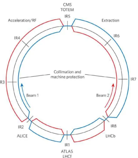
II Accelerate and Collide 27 3 Large Hadron Collider 29 3.1 Performance Goals . . . 29
3.3 Nominal Luminosity and Beam Parameters . . . 32 3.4 Lattice Layout . . . 33 3.5 LHC Collision Detectors . . . 34 3.5.1 Pile-up Events . . . 34 3.5.2 Collision Rate . . . 35 3.5.3 High Radiation . . . 35 3.6 Operation from 2010 to 2012 . . . 35
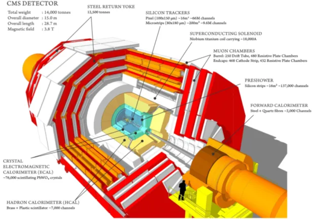
4 Compact Muon Solenoid 37 4.1 CMS Detector and its Magnet . . . 37
4.2 Coordinate System . . . 38
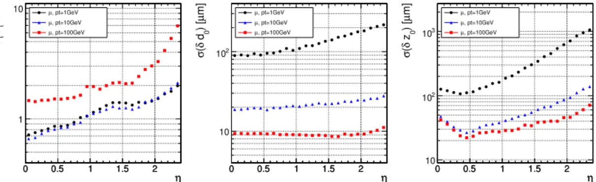
4.3 Inner Tracking System . . . 40
4.4 Electromagnetic Calorimeter . . . 42
4.4.1 ECAL Crystals and Geometry . . . 43
4.4.2 Photodetectors . . . 45
4.4.3 Preshower . . . 46
4.4.4 Laser Monitoring . . . 46
4.4.5 Detector Calibration . . . 47
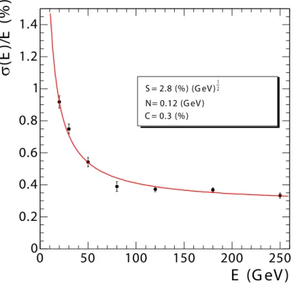
4.4.6 Energy Resolution . . . 47
4.4.7 Position Resolution and Alignment . . . 49
4.5 Hadron Calorimeter . . . 49
4.6 Muon System . . . 51
4.6.1 Drift Tube Chambers . . . 51
4.6.2 Cathode Strip Chambers . . . 52
4.6.3 Resistive Plate Chambers . . . 52
4.6.4 Muon Momentum Resolution . . . 53
4.7 Trigger and Data Acquisition . . . 53
4.7.1 Level-1 Trigger Architecture . . . 54
4.7.2 High-Level Trigger Architecture . . . 57
4.7.3 The Data Acquisition System . . . 58
4.8 Leptons Signature in CMS . . . 59
4.8.1 Electrons . . . 59
4.8.2 Muons . . . 60
III Choose Building Blocks 63 5 Datasets and Triggers 65 5.1 Collision Data . . . 65
5.2 Simulated Samples . . . 67
5.2.1 Signal: H → ZZ(∗)→ 4ℓ . . . . 69
5.2.2 Background: q ¯q → ZZ(∗)→ 4ℓ . . . . 71
Contents
5.2.4 Background: Z+jets→ 2ℓ+jets . . . . 72
5.2.5 Background: t ¯t → 2ℓ2ν2b . . . . 72
6 Leptons and Photons 73 6.1 Electrons . . . 74 6.1.1 Reconstruction . . . 74 6.1.2 Identification . . . 84 6.2 Muons . . . 91 6.2.1 Reconstruction . . . 91 6.2.2 Identification . . . 92 6.3 Lepton Isolation . . . 94 6.3.1 Pile-up Subtraction . . . 98
6.3.2 Working Point Optimization . . . 102
6.4 Leptons common Vertex . . . 104
6.5 Photons . . . 104
6.5.1 Photon Observables and FSR Recovery . . . 104
6.5.2 Photon Reconstruction, Identification and Isolation . . . 105
6.5.3 Building Z bosons with FSR Photon Recovery . . . 106
6.5.4 Performance of FSR Photon Recovery . . . 107
7 Lepton Selection Validation from Data 111 7.1 Tag-and-probe Method . . . 111
7.2 Electron measurements . . . 113
7.2.1 Reconstruction . . . 114
7.2.2 Identification . . . 116
7.2.3 Isolation and Impact Parameter . . . 116
7.2.4 Trigger . . . 122
7.2.5 Electron Scale Factors . . . 124
7.3 Muon Measurements . . . 130
7.3.1 Reconstruction and Identification . . . 130
7.3.2 Impact Parameter . . . 131
7.3.3 Isolation . . . 131
7.3.4 Trigger . . . 131
IV Come Together 133 8 Analysis Strategy and Event Selection 135 8.1 General Analysis Strategy . . . 136
8.2 Event Selection . . . 138
8.2.1 Trigger Selection . . . 139
8.2.2 Lepton Selection . . . 139
8.2.3 Final Selection and Combinatorics . . . 140
9 Signal Modelling and Uncertainties 147
9.1 Signal Model at Low Masses . . . 148
9.2 Signal Model at High Masses . . . 150
9.2.1 Lineshape with Complex Pole Scheme . . . 150
9.2.2 Evaluation of the High-mass Corrections Systematic Uncertainties . . . 152
9.2.3 High Higgs Boson Mass Signal Model . . . 152
9.3 Signal Model Uncertainties . . . 154
9.3.1 Theoretical Uncertainties . . . 154
9.3.2 Data-to-MC Scale Factors from Efficiencies . . . 157
9.3.3 Four-lepton mass Scale and Resolution . . . 160
9.4 Event-by-event Mass Errors . . . 166
9.4.1 Calibration of Per-event Mass Errors . . . 167
9.4.2 Expectations from Simulation . . . 168
9.4.3 Validation of Per-event Mass Errors from Data . . . 170
9.5 Event-by-event Mass Errors Model . . . 175
10 Reducible Background Modelling and Uncertainties 177 10.1 Reducible Background Estimation . . . 177
10.2 Methodology . . . 178
10.2.1 Results on Data . . . 183
10.2.2 Alternative Method . . . 183
10.3 Reducible Background Uncertainties . . . 184
10.3.1 Statistics in 4ℓ control sample . . . 185
10.3.2 Functional form for m4ℓshape . . . 185
10.3.3 Closure Test with Z and Opposite Flavor Leptons . . . 186
10.4 Reducible Background Summary . . . 186
11 Irreducible Background Modelling and Uncertainties 189 11.1 ZZ(⋆)Background Model . . . 190
11.2 ZZ(⋆)Background Model Uncertainties . . . 193
11.2.1 Theoretical Uncertainties . . . 193
12 Kinematic Discriminant 197 12.1 Methodology . . . 197
12.2 Construction of MELA Discriminant . . . 199
12.3 Parametrization of MELA Discriminant . . . 203
12.4 MELA for Spin-Parity Properties Measurements . . . 205
13 Statistical Analysis 211 13.1 Methodology of using 2D Distributions . . . 211
13.2 Methodology of using 3D Distributions . . . 215
Contents
V Bingo! 223
14 Final Results 225
14.1 Summary of Selection and Systematic Uncertainties . . . 225
14.1.1 Event Yields . . . 225 14.1.2 Event Distributions . . . 228 14.1.3 Systematic Uncertainties . . . 234 14.2 Exclusion Limits . . . 236 14.3 Significance of Excesses . . . 238 14.4 Mass Measurement . . . 240
14.5 Spin and Parity Measurements . . . 242
Conclusions 245
Appendix 247
A ECAL Energy Measurement with Multivariate Regression 249
B Tag-and-probe Measurements 253
References 273
Introduction
To express the complexity of the Universe with a handful of fundamental laws is absolutely es-sential if one wishes to understand the phenomena within the matter and the space enclosing us. While the trial of formulating these relations must be as old as the spoken word, it needed the formalism of natural science in general and mathematics in particular to reward these trials with success—success in a twofold manner. First, only the mathematical formulation of phenomena allows a quantification and thus a verification against measured observations, second, it can in general be understood and tested by anyone.
Together with the deployment of the scientific method, the idea that matter is built up from a limited set of elementary components was developed. The idea that the profound constituents are the elements water, fire, earth and air was stated by the Greek philosopher Empedocles five centuries B.C.. Shortly after Leucippus and Democritus established the principle that all matter is formed by extremely small, fundamental and indestructible particles, that they called atoms. The idea of the atoms was picked up by scientists in the 19t hcentury, but only in the year 1909, with the experiment of Ernest Rutherford, it became clear that the atoms have structure. Furthermore, with the discovery of the neutron by James Chadwick in 1932 it was established that the nucleus itself is composed of smaller particles.
In the 50’s and 60’s of the 20t h century a several particle physics experiments showed that there are many more particles with characteristics similar to the protons and neutrons. It was believed that they themselves are not fundamental, but formed by even smaller particles, the
quarks. The quark model, whose convincing confirmation was the discovery of point-like
constituents of the protons in 1969, allowed to classify all the known hadrons as compound objects of two or three quarks.
In parallel to the search for the elements of matter, the question on their interaction was posed. The work of James Clerk Maxwell was pioneering in this regard. He discovered unique fundamental mechanism behind the electricity and magnetism phenomena—the
electro-magnetism. This observation was formed in a set of equations—the Maxwell equations, which,
together with the discovery of the quantum nature of physics and special relativity, formed later the extremely successful theory of Quantum Electrodynamics (QED).
as a template, the endeavor was set to describe the other forces, the weak force responsible for the decay of nuclei and the strong force, responsible for the formation of discovered hadrons. It was found that the strong interaction can be formulated as a relativistic field-theory of colour charged quarks and gluons, known as Quantum Chromodynamics (QCD). The weak force could be combined with QED into the so called electroweak interaction, also known as Glashow-Weinberg-Salam (GWS) model. The GWS theory together with QCD form the current most successful theory for the interaction of elementary particles, referred to as the Standard Model (SM) of Particle Physics.
In general in such theories, known as Gauge Theories, the particles responsible for the action of the force, the gauge or vector bosons, as well as elementary fermions, have to be massless. However, experiments showed that the particles responsible for the weak interaction are very massive. Elementary matter particles also have masses. A mechanism, the so-called Brout-Englert-Higgs (BEH) mechanism has been proposed to remedy the theory deficiency. This mechanism, developed and published in 1964 by Peter Higgs, Robert Brout and Francois Englert, postulates the existence of a new scalar field responsible for electroweak symmetry breaking (EWSB), the Higgs field. The gauge bosons acquire mass. The fermions become massive by interacting via Yukawa interactions with the Higgs field. The theory predicts the existence of a physical scalar boson, the Higgs boson.
A variety of tests and precision measurements over the last decades gave very strong confi-dence in the Standard Model, in particular the prediction and discovery of particles like Z boson and top quark. The discovery of the Higgs boson, the only missing piece, would be (is) the unprecedented achievement of the Standard Model.
The mass of the Higgs boson, the quanta of the Higgs field is not predicted by the mechanism, thus it has to be experimentally deduced. The existence of an elementary particle such as the Higgs boson is tested at colliders. High energy collisions are aimed to create the searched particle, and detectors embedded around collision points allow to seek for a typical signature. After the exclusions from the Large Electron Positron Collider (LEP) and the Tevatron experiments, the Large Hadron Collider (LHC) become the major actor for the Higgs hunting and possibly taming in the full mass range allowed by the theory.
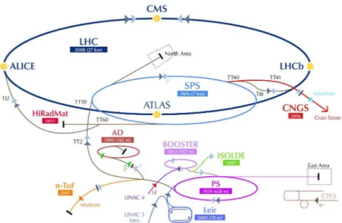
The development and construction of the LHC machine took over two decades. It was built to provide proton-proton collisions with a nominal centre of mass energy of 14 TeV (7 TeV and 8 TeV during the first years) and a very high luminosity. In parallel, detectors were designed and built, responding to the LHC characteristics and the physics goals. In particular the Compact Muon Solenoid (CMS) and A Toroidal LHC Apparatus (ATLAS) experiments were primarily set to search for the Higgs boson in a wide variety of production and decay channels. The response of the detectors has been simulated with great care, facilitating the development of physics object reconstruction and research analysis.
This thesis work started with the very first collisions at the LHC at the end of 2009. By spring 2010, the LHC reached working conditions for the physics with an energy in the centre of mass
of the proton-proton collisions of 7 TeV. I was involved in the commissioning of basic objects for the reconstruction of the collision events, and in particular of the electrons.
At that time, I also took part in the deployment of the analysis strategy for the search of the Higgs boson, specifically in the determination of the discriminating observables as well as definition of Higgs boson mass-dependent search phase space. The search relies solely on the measurement of leptons achieving high reconstruction, identification and isolation efficiency for a ZZ → 4ℓ system. The ZZ system is composed of two same-flavour and opposite-charge isolated leptons, e+e−andµ+µ−in the mass range m4ℓ> 100 GeV. One or both of the Z bosons
can be off-shell. The background sources include an irreducible four-lepton contribution from direct ZZ (or Zγ) production via q ¯q annihilation and g g fusion. Reducible contributions arise
from Z b ¯b and t ¯t where the final states contain two isolated leptons and two b jets producing
secondary leptons. Additional background of instrumental nature arises from Z + jets events where jets are misidentified as leptons.
In the following months, LHC was constantly increasing luminosity accelerating the collection of data. The increase of luminosity resulted in multiple collisions in a single bunch crossing, the so-called pile-up. To ensure the robustness of measured quantities, especially lepton isolation, a correction method using the average energy density deposited by the emerging particles has been deployed. The method is known as effective area correction and is currently used across many analysis in CMS. By the international conferences of the summer 2011, enough data had been collected to produce the first comprehensive search for the Higgs boson at the LHC and it was becoming clear that this simple and robust analysis had to be expanded to better cover the very low mass range.
This thesis describes the analysis as it was developed and deployed starting in fall 2011 with increased acceptance for Higgs boson in the low mass range. This implied even more demand-ing conditions on low pT leptons, which presupposes a good control of lepton measurements.
This work was carried out using the tag-and-probe method which uses Z decays as a handle to extract the possible differences between collision data and simulation. In addition, an effort was made to extract the maximum amount of information from events, using per-event mass uncertainties and, starting from spring 2012, exploiting the discriminating power from the full decay kinematics.
The thesis is divided into five parts. Part one, “Breaking the Symmetry”, is dedicated to theo-retical aspects of Higgs boson phenomenology at hadron colliders. After a brief introduction to Standard Model in chapter 1, with focus on the BEH mechanism, we turn in chapter 2 to the relevant Higgs production processes and decay modes at LHC.
Part two, “Accelerate and collide”, gives a short overview of the experimental apparatus, the CMS detector at the LHC. A slight accent has been put on the electromagnetic calorimetry as it is one of the key components in the electron reconstruction and measurements.
discussion on simulation and collision data choice for the analysis in the chapter 5, we quickly move to a detailed overview of physics objects—electrons, muons and photons—in chapter 6. An emphasis is put on electron reconstruction, identification and particularly isolation being one of the main topics I have been working on. In this very chapter, we also define the final state radiation (FSR) recovery strategy which has been put in place for the 2012 analysis. Bearing in mind that we have four leptons in final state, it is hard to overemphasize the importance of lepton selection efficiency measurements using data-driven techniques. These are presented in chapter 7.
Having chosen the building blocks, we try to make them “Come together” in part four. We start in chapter 8 by carefully defining the analysis strategy which would allow for a graduate decent into the signal phase space and a good control of background rates. Since the search for a Higgs boson in four-lepton channel is a hunt for a resonance in the four-lepton invariant mass parameter space, it is beneficial to model the signal yields, shapes and efficiencies, as well as background ones with respect to mass. These models are then used as inputs for the final statistical analysis. A detailed discussion of signal and background models is presented in chapters 9, 10 and 11. In chapter 12 we shed light on the full kinematic discriminant which complements the four-lepton mass measurement and increase the sensitivity of the search. “Bingo!”—the title says it all. In this part we present the final statistical analysis and results
for the exclusion limits and significances of event excesses in the four-lepton invariant mass spectrum. In addition, we bring a strategy to measure the Higgs boson spin-parity properties. The boson discovery at mass around 125 GeV—although in this channel only observation—was announced on a memorable CERN seminar in Geneva on 4t hJuly 2012 by CMS spokesperson Joseph Incandela. Quickly afterwards, the analysis was published in a prestigious journal— Physics Letters B [1].
“Bingo!”—the title says it all. In this part we present the final statistical analysis and results for the exclusion limits and significances of event excesses in the four-lepton invariant mass spectrum. Evidence was found for the existence of a new boson around 125 GeV from the H → ZZ(⋆)→ 4ℓ channel, and, combined with the H→ γγ channel, led to the observation by CMS. Similar observations were obtained simultaneously by the ATLAS experiment. The discovery of a new boson was announced on a memorable CERN seminar in Geneva on the 4thof July 2012 by the CMS spokesperson, Joe Incandela, and the ATLAS spokesperson, Fabiola Gianotti. Quickly afterwards, the analysis was published in a prestigious journal—Physics Letters B [1]. More data was analysed in the H → ZZ(⋆)→ 4ℓ in fall 2012 and the first spin-parity measurements performed by the CMS experiment have been published in another prestigious journal, Physics Review Letters. All these results are described in this thesis.
Part I
1
The Standard Model
The fundamental components of matter and their interactions are nowadays best described by the Standard Model of Particle Physics (SM), which is based on two complementary quantum field theories, describing the electroweak interaction (Glashow-Weinberg-Salam model or GWS) and the strong interaction (Quantum Chromodynamics or QCD). The gauge group of the Standard Model is SU (3)C⊗ SU (2)L⊗U (1)Y, where SU (2)L⊗U (1)Y are related to the
cou-plings of the electroweak interaction, whilst SU (3)Cis related to gauge couplings in quantum
chromodynamics. In this chapter, a short overview of the electroweak theory (Sec. 1.2) is given, focusing the attention on the EWSB, the Higgs mechanism and the Higgs boson (Sec. 1.3). In subsequent chapter we will set the theoretical landscape for the Higgs boson searches performed at the LHC by introducing the relevant production and decay modes of the boson. Note that natural units will be used, i.e.~= c = 1, unless otherwise specified.
1.1 The Standard Model of Elementary Particles
The SM describes the matter at the physical level as composed by 3 families of 4 elementary particles, which are fermions with spin 1/2. Ordinary matter is composed only of the 1st family members, and other two families can be regarded as the replicas of the first one. The corresponding particles belonging to separate families are said to have different flavours, with same coupling constants but with different masses. The fermions can be divided into two main groups, leptons and quarks, whose classification is given in Table 1.1. Quarks are subject to both strong and electroweak interactions and do not exist as free states, but only as constituents of a wide class of particles, the hadrons, such as protons and neutrons. Leptons, instead, only interact by electromagnetic and weak forces.
In the SM, the interactions between particles are described in terms of the exchange of bosons, integer-spin particles which are carriers of the fundamental interactions. The main character-istics of bosons and corresponding interactions are summarized in Table 1.2 (the gravitational interaction is not taken into account, as it is not relevant at the scales of mass and distance
Fermions 1stfam. 2ndfam. 3rdfam. Charge Interactions Quarks u d c s t b +23 −13 all Leptons e νe µ νµ τ ντ −1 0 weak, electromagnetic weak
Table 1.1: Classification of the three families of fundamental fermions.
typical of the particle physics).
Electromagnetic Weak Strong
Quantum Photon (γ) W±, Z Gluons
Mass [GeV] 0 80–90 0 Coupling constant α(Q 2 = 0) ≈1371 GF≈ 1.2 · 10−5GeV−2 αs(mZ) ≈ 0.1 Range [cm] ∞ 10−16 10−13
Table 1.2: Fundamental interactions relevant in particle physics and corresponding carriers.
As previously mentioned, the SM describes these interactions by means of two gauge theories: the Quantum Chromodynamics and the theory of the electroweak interaction (Glashow-Weinberg-Salam model), which unifies the electromagnetic and weak interactions. Since the present work deals with a purely electroweak decay, in the next sections only the latter theory will be described in some detail.
1.2 The Electroweak Theory
From a historical point of view, the starting point for the study of electroweak interactions is Fermi’s theory of muon decay [2], which is based on an effective four-fermion Lagrangian1:
L = −4GpF 2ν¯µγ α1 − γ5 2 µ ¯eγα 1 − γ5 2 νe, (1.1)
with GF≃ 1.16639 × 10⁻⁵GeV−2. Eq. 1.1 represents a “point like” interaction, with only one
vertex and without any intermediate boson exchanged. It is usually referred to as a V − A interaction, being formed by a vectorial and an axial component. The term 12(1 − γ5) that
appears in it is the negative chirality projector. Only the left-handed components of fermions takes part to this effective interaction.
Fermi’s Lagrangian is not normalizable and it results in a non-unitary S matrix. Both
1.2. The Electroweak Theory
malizability and unitarity problems can be overcome by describing the weak interaction with a gauge theory, i.e. requiring its Lagrangian to be invariant under local transformations generated by the elements of some Lie group (gauge transformations). The specific group of local invariance (gauge group) is to be determined by the phenomenological properties of the interaction and of the particles involved. In particular, the resulting Lagrangian must reduce to Eq. 1.1 in the low energy limit. A detailed derivation of this Lagrangian is not provided here, but the results are summarized in the following (for details about the GWS model, see Refs. [3, 4, 5]).
A gauge theory for weak interactions is conceived as an extension of the theory of electro-magnetic interaction, the QED, which is based on the gauge group U (1)E M, associated to the
conserved quantum number Q (electric charge). In this case, the condition of local invariance under the U (1)E Mgroup leads to the existence of a massless vector field, the photon.
A theory reproducing both the electromagnetic and weak interaction phenomenology is achieved by extending the gauge symmetry to the groupSU (2)I⊗U (1)Y. In this sense, the
weak and electromagnetic interactions are said to be partially unified. The generators of
SU (2)I are the three components of the weak isospin operator, ta=12τa, whereτa are the
Pauli matrices. The generator of U (1)Y is the weak hypercharge Y operator. The corresponding
quantum numbers satisfy
Q = I3+
Y
2,
where I3is the third component of the weak isospin (eigenvalue of t3).
Fermions can be divided in doublets of negative chirality (left-handed) particles and singlets of positive chirality (right-handed) particles, as follows:
LL= Ã νℓ,L ℓL ! , ℓR QL= Ã uL dL ! , uR, dR, (1.2)
whereℓ = e,µ,τ, u = u,c, t and d = d, s,b. Chirality is not to be confused with helicity. Helicity
coincides with chirality only for massless particles (e.g. the neutrino2), since it is not possible to make Lorentz transformation which would result with reversing the orientation of the momentum vector, since their velocity always equals c. For massive particles, one can change helicity by changing the Lorentz frame—chirality however is the intrinsic property of the particle, independent of the frame of reference.
In Table 1.3, I3, Y and Q quantum numbers of all fermions are reported.
The requirement of local gauge invariance is one of the most fascinating concepts in quantum field theories as it implies the very existence of the fundamental interactions. Inspired by QED, imposing the requirement of local gauge invariance with respect to the SU (2)IxU (1)Y group
alone introduces four massless vector fields, Wµ1,2,3and Bµ, which couple to fermions with
I3 Y Q µ uL dL ¶ µ 1 2 −12 ¶ µ 1 3 1 3 ¶ µ 2 3 −13 ¶ uR, dR 0, 0 43, −23 23, −13 µ νℓ,L ℓL ¶ µ 1 2 −12 ¶ µ −1 −1 ¶ µ 0 −1 ¶ ℓR 0 −2 −1
Table 1.3: Isospin (I3), hypercharge (Y ) and electric charge (Q) of the fermions in the 1stfamily. Other
two families are exact replicas of the first one.
two different coupling constants, g and g′.
Notice that Bµdoes not represent the photon field, because it arises from the U (1)Y group of
hypercharge, instead of U (1)E Mgroup of electric charge. The gauge-invariant Lagrangian for
fermion fields can be written as follows: L = ΨLγµ ³ i∂µ+ g taWµa−12g′Y Bµ ´ ΨL+ ψRγµ¡i ∂µ−12g′Y Bµ¢ ψR (1.3) where ΨL= à ψ1L ψ2L !
and whereΨLandψRare summed over all the possibilities in Eq. 1.2.
As already stated, Wµ1,2,3and Bµdo not represent physical fields, which are given instead by
linear combinations of the four mentioned fields: the charged bosons W+and W−correspond to3 Wµ±= r 1 2(W 1 µ∓ iWµ2), (1.4)
while the neutral bosonsγ and Z correspond to
Aµ = BµcosθW+Wµ3sinθW (1.5)
Zµ = −BµsinθW+Wµ3cosθW, (1.6)
obtained by mixing the neutral fields Wµ3and Bµwith a rotation defined by the Weinberg angle
θW. In terms of the fields in Eqs. 1.4 and 1.6, the interaction term between gauge fields and
fermions, taken from the Lagrangian in Eq. 1.3, becomes Li nt= 1 2p2g (J + αW(+)α+ J−αW(−)α) + 1 2 q g′2+ g2JZ αZα− e JαE MAα, (1.7) 3W(−)
1.3. The Brout-Englert-Higgs Mechanism
where JE Mis the electromagnetic current coupling to the photon field, while J+, J−and JZ are the three weak isospin currents. It is found that
JαZ= Jα3− 2sin2θW· JαE M.
Aµcan then be identified with the photon field and, requiring the coupling terms to be equal,
one obtains
g sinθW = g′cosθW = e (1.8)
which represents the electroweak unification. The GWS model thus predicts the existence of two charged gauge fields, which only couple to left-handed fermions, and two neutral gauge fields, which interact with both left- and right-handed components.
1.3 The Brout-Englert-Higgs Mechanism
In order to correctly reproduce the phenomenology of weak interactions, both fermion and gauge boson fields must acquire mass, in agreement with experimental results. Up to this point, however, all particles are considered massless: in the electroweak Lagrangian, in fact, a mass term for the gauge bosons would violate gauge invariance4, which is needed to ensure the renormalizability of the theory.
There must be something external to the fundamental fields fermions and gauge boson fields of the theory to generate the mass of the particle while preserving the local gauge symmetry which is at the very origin of the existence of interactions. In the Standard Model this is achieved by postulating the existence of a new field, a scalar field—the so-called Higgs field, which is needed to ensure the renormalizability of the theory. Masses are thus introduced with the so-called BEH mechanism [6, 7, 8, 9, 10, 11], which allows fermions and W±, Z bosons to be massive5, while keeping the photon massless. Such mechanism is accomplished by means of a doublet of complex scalar fields
φ = Ã φ+ φ0 ! =p1 2 Ã φ1+ i φ2 φ3+ i φ4 ! , (1.9)
which is introduced in the electroweak Lagrangian within the term
LEW SB= (Dµφ)†(Dµφ) +V (φ†φ), (1.10)
where Dµ= ∂µ− i g taWµa+i2g′Y Bµis the covariant derivative. The Lagrangian in Eq. 1.10 is
invariant under SU (2)I⊗U (1)Y transformations, since the kinetic part is written in terms of
4Explicit mass terms for fermions would not violate gauge invariance, but in the GWS model the Lagrangian
is also required to preserve invariance under chirality transformations, and this is achieved only with massless fermions.
5Rigorously speaking, the BEH mechanism is only needed to explain how W±and Z acquire their mass. A
covariant derivatives and the potential V only depends on the productφ†φ. The φ field is
characterized by the following quantum numbers:
I3 Y Q Ã φ+ φ0 ! Ã 1 2 −12 ! Ã 1 1 ! Ã 1 0 !
Writing the potential term as follows (see also Fig. 1.1)
V (φ†φ) = −µ2φ†φ − λ(φ†φ)2, (1.11) where the choice ofµ2> 0 and λ > 0 leads to a very interesting shape of the potential, crucial
for the BEH mechanism. Such a choice of the potential, shown in Fig. 1.1, has a minimum for
φ†φ =1 2(φ 2 1+ φ22+ φ23+ φ24) = − µ2 2λ≡ v2 2 . (1.12)
This minimum is not found for a single value ofφ, but for a manifold of non-zero values. The
choice of (φ+,φ0) corresponding to the ground state (i.e. the lowest energy state, or vacuum)
is arbitrary and the chosen point is not invariant under rotations in the (φ+,φ0) plane: this is referred to as spontaneous symmetry breaking. If one chooses to fix the ground state on theφ0
axis, the vacuum expectation value of theφ field is
〈φ〉 =p1 2 Ã 0 v ! , v2= −µ 2 λ. (1.13)
Figure 1.1: Shape of the Higgs potential of Eq. 1.11.
Theφ field can thus be rewritten in a generic gauge, in terms of its vacuum expectation value: φ =p1 2e i vφ at a à 0 H + v ! , a = 1,2,3
where the three fieldsφa and the fourthφ4= H + v are called Goldstone fields. Being scalar and massless, they introduce four new degrees of freedom, in addition to the six degrees due to the transverse polarizations of the massless vector bosons W±and Z . The unitary gauge is
1.3. The Brout-Englert-Higgs Mechanism
fixed by the transformation
φ′= e−viφ at aφ = 1 p 2 Ã 0 H + v ! =p1 2 Ã 0 φ4 ! .
The remaining field, the Higgs field, has now a zero expectation value.
Rewriting the Lagrangian in Eq. 1.10 with theφ field in the unitary gauge, LEW SBresults from
the sum of three terms:
LEW SB= LH+ LHW+ LH Z, (1.14)
where the three terms can be written as follows, using the approximation V ∼ µ2H2+ cost
and neglecting higher order terms: LH = 1 2∂αH∂ α H + µ2H2 LHW = 1 4v 2g2W αW†α+ 1 2v g 2HW αW†α (1.15) = mW2 WαW†α+ gHWHWαW†α LH Z = 1 8v 2(g2 + g′2)ZαZα+ 1 4v(g 2 + g′2)H ZαZα (1.16) = 12m2ZZαZα+ 1 2gH ZH ZαZ α.
Eqs. 1.15 and 1.16 now contain mass terms for W±and Z : each of the three gauge bosons has acquired mass and an additional degree of freedom, corresponding to the longitudinal polarization. At the same time, three of the four Goldstone bosons have disappeared from the Lagrangian LEW SB, thus preserving the total number of degrees of freedom: the degrees
linked to the missing Goldstone bosons have become the longitudinal degrees of the vector bosons. A scalar boson, the so-called Higgs boson associated to the Higgs field is present as a new massive particle in the theory. The mass of the Higgs boson which is presumed to be related to self-interactions of the field is not predicted by the theory.
In summary, the BEH mechanism is used to introduce the weak boson masses without ex-plicitly breaking the gauge invariance and thus preserving the renormalizability of the theory. When a symmetry is “spontaneously” broken, in fact, it is not properly eliminated—it is rather “hidden” by the choice of the ground state. In practice, this means that physical bosons can now be massive despite the fact that the fundamental gauge bosons of the theory remain massless. In addition, not only bosons, but all other particles acquire their mass through the interaction with Higgs field. It can be shown that the minimum for the Higgs field is still invariant for the U (1)E Mgroup: the electromagnetic symmetry is therefore unbroken and the
1.3.1 Vector Boson Masses and Couplings
Equations 1.15 and 1.16 show that the masses of vector bosons W±and Z are related to the parameter v,the vacuum expectation value (VEV) which sets a characteristic mass scale for the EWSB, and to the electroweak coupling constants:
( mW=12v g mZ=12vpg2+ g′2 → mW mZ = g pg2+ g′2 = cosθW. (1.17)
Also the couplings of vector bosons to the Higgs can be obtained from Eqs. 1.15 and 1.16 and are found to depend on the square of mW and mZ:
gHW= 1 2v g 2 =2 vm 2 W (1.18) gH Z= 1 2v(g 2 + g′2) =2 vm 2 Z. (1.19)
A relation between decay ratios of Higgs boson to a W pair and to a Z pair can be derived from Eqs. 1.18 and 1.19: B R(H → W+W−) B R(H → Z Z ) = Ã gHW 1 2gH Z !2 = 4Ã m 2 W m2Z !2 ∼ 2.4.
Finally, the characteristic mass scale for EWSB can be determined from the relation between the v parameter and the Fermi constant GF:
v = µ 1 p 2GF ¶1 2 ≃ 246 GeV. (1.20)
1.3.2 Fermion Masses and Couplings
The Higgs mechanism is also used to generate the fermion masses, by introducing in the SM Lagrangian a SU (2)I⊗ U (1)Y invariant term (called Yukawa term) that represents the
interaction between the Higgs and the fermion fields. Sinceφ is an isodoublet, while the
fermions are divided in left-handed doublet and right-handed singlet, the Yukawa terms (one for each fermion generation) must have the following expression for leptons:
Lℓ= −GHℓ· lℓφℓR+ ℓRφ†lℓ.
In the unitary gauge, the first component ofφ is zero, therefore a mass term will arise from the
Yukawa Lagrangian only for the second component of lℓ: this correctly reproduces the fact
that neutrino is (approximately) massless. Lℓ= −GpHℓ
2 vℓℓ −
GHℓ
p
1.3. The Brout-Englert-Higgs Mechanism
For what concerns the quark fields, the down quarks (d , s, b) are treated in the same way as leptons; up quarks (u, c, t ), instead, must couple to the charge-conjugate ofφ
φc= −i τ2φ∗= 1 p 2 Ã φ3− i φ4 −φ1+ i φ4 ! ,
which becomes in the unitary gauge
φc=p1 2 Ã η + v 0 ! .
The Yukawa Lagrangian will be therefore
LY = −GHℓLLφℓR−GH dQLφdR−GHuQLφcuR+ h.c.. (1.22) From Eq. 1.21, the mass of a fermion (apart from neutrinos) and its coupling constant to the Higgs boson are found to be
mf = GH f p 2 v (1.23) gH f = GH f p 2 = mf v . (1.24)
Being the GH f free parameters, the mass of the fermions cannot be predicted by the theory.
At this point we can understand more deeply what the fermion mass terms in the Lagrangian really means. The interaction with the Higgs field transform a right-handed chirality in a left-handed chirality (and vice versa) such that the physical object becomes a massive particle. The mass term is therefore only measure of the strength of the interaction of particle with Higgs field.
This analysis is somewhat illustrative, since it does not take account of the fact that in reality there are three families of quarks and leptons. Complete analysis would be more complicated, since the weak mass eigenstates are not the same as the physical mass eigenstates. If one wants to deal with the physical particles, one needs to make transformation from the weak mass basis to physical mass bases. This is accomplished by the usual unitary transformation matrices, Cabibbo–Kobayashi–Maskawa (CKM) and Pontecorvo–Maki–Nakagawa–Sakata (PMNS) matrices, for quark and lepton sectors respectively.
1.3.3 Higgs Boson Mass
Among the 18 free parameters of the SM6, the Higgs boson mass is the only still undetermined one. Although the Higgs boson mass is not predicted by the theory, the assumption that the Higgs boson acquires a mass, e.g. via self-interactions of the Higgs field, is essential for the EWSB mechanism,i.e. without the mass of the Higgs, there would be no ”Mexican hat” potential. Its mass depends on the parameters v andλ, but while the former can be estimated
by its relation with the GF constant of Fermi’s theory, the latter is characteristic of the field
φ and cannot be determined other than measuring the Higgs mass itself. However, both
theoretical and experimental constraints exist, including those from direct search at colliders, in particular LEP.
Theoretical Constraints
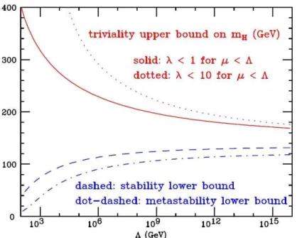
Theoretical constraints to the Higgs mass value [13] can be found by imposing the energy scaleΛ up to which the SM is valid, before the perturbation theory breaks down and non-SM phenomena emerge. The upper limit is obtained by requiring that the running quartic coupling of Higgs potentialλ remains finite up to the scale Λ (triviality). A lower limit is found
instead by requiring thatλ remains positive after the inclusion of radiative corrections, at least
up toΛ: this implies that the Higgs potential is bounded from below, i.e. the minimum of such potential is an absolute minimum (vacuum stability). A looser constraint is found by requiring such minimum to be local, instead of absolute (metastability). These theoretical bounds on the Higgs mass as a function ofΛ are shown in Fig. 1.2.
If the validity of the SM is assumed up to the Planck scale (Λ ∼ 1019GeV), the allowed Higgs mass range is between 130 and 190 GeV, while forΛ ∼ 1 TeV the Higgs mass can be up to 700 GeV. On the basis of these results, however, colliders should look for the Higgs boson up to masses of ∼ 1 TeV. If the Higgs particle is not found in this mass range, then a more sophisticated explanation for the EWSB mechanism will be needed.
Very important limits come from the requirement of the unitarity of S-matrix, which basically can be reduced to the claim that scattering probability cannot exceed the value of 100%. In order to avoid violation of unitarity, the Higgs boson plays crucial role, since this very concept allows us to regulate the unitarity of S-matrix asΛ increases.
Experimental Constraints
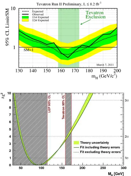
Bounds on the Higgs mass are also provided by electroweak precision measurements at LEP, SLC and Tevatron [14] (updated in 2010). Direct searches at LEP-II have set the limit
mH> 114.4 GeV (95% C.L.) [15] and those performed at Tevatron have excluded the mass
69 fermion masses (+ 3 neutrino masses, if m
ν6= 0), 3 CKM mixing angles + 1 phase (+ 3 more angles + 1
additional phase for neutrinos), the electromagnetic coupling constantαE M, the strong coupling constantαS, the
1.3. The Brout-Englert-Higgs Mechanism
Figure 1.2: Red line: triviality bound (for different upper limits toλ); blue line: vacuum stability (or
metastability) bound on the Higgs boson mass as a function of the new physics (or cut-off ) scaleΛ [13].
range 158 < mH< 175 GeV also at 95% C.L. [16](see Fig. 1.3 left). Moreover, since the Higgs
boson contributes to radiative corrections, many electroweak observables are logarithmically sensitive to mH and can thus be used to constrain its mass. All the precision electroweak
measurements performed by the four LEP experiments and by SLD, CDF and D; have been combined together and fitted [17], assuming the SM as the correct theory and using the Higgs mass as free parameter. The result of this procedure is summarized in Fig. 1.3 (b), where ∆χ2= χ2− χ2mi nis plotted as a function of mH.
The solid curve is the result of the fit, while the shaded band represents the theoretical un-certainty due to unknown higher order corrections. The indirectly measured value of the Higgs boson mass, corresponding to the minimum of the curve, ismH= 91+30−23GeV at 68%
confidence level (CL). This value correspond to the black line in Fig. 1.3 and does not take the theoretical uncertainties into account. The indirect constraints thus favour a low mass value for the the Higgs boson. But the dependence on the Higgs boson mass of the indirect constraints is only logarithmic such that the central value must be interpreted with care. It remains essential to search for a SM Higgs boson over the full mass range allowed by the theory.
Such results are model-dependent, as the loop corrections take into account only contribu-tions from known physics. This result is thus well-grounded only within the SM theory and has always to be confirmed by the direct observation of the Higgs boson.
Figure 1.3: (a) 2011 Tevatron exclusion at 95% C.L. in Higgs boson mass range from 158 to 172 GeV.
(b)∆χ2of the fit to the electroweak precision measurements of LEP, SLC, and Tevatron as a function of the Higgs mass (2012). The solid (dashed) lines give the results when including (ignoring) theoretical errors. The gray area represents the region excluded by direct searches at LEP and Tevatron.
2
Higgs Boson Search at the LHC
The experiments at the LHC are searching for the SM Higgs boson within the full mass range allowed by the theory given unitary and above LEP constraints, i.e. from 114 up to about 800 GeV to 1 TeV. In the work described by this thesis, the analysis has been performed up to 800 GeV. In this chapter, the main Higgs production and decay processes are described. This will allow to identify the most promising channels in the perspective of a Higgs boson discovery.
While the Higgs mass is not predicted by the theory, the Higgs couplings to the fermions or bosons are predicted to be proportional to the corresponding particle masses for fermions or squared masses for bosons, as in Eqs. 1.18, 1.19 and 1.24. For this reason, the Higgs production and decay processes are dominated by channels involving the coupling of Higgs to heavy particles, mainly to W±and Z bosons and to the third generation fermions. For what concerns
the remaining gauge bosons, the Higgs does not couple to photons and gluons at tree level, but only by one-loop graphs where the main contribution is given by q ¯q and by W+W−loops.
2.1 Higgs Production
The main processes contributing to the Higgs production at a hadron collider are represented by the Feynman diagrams in Fig. 2.1 and the corresponding cross-sections for proton-proton centre of mass energies ofps = 7 TeV andps = 8 TeV, adopted by the LHC, are shown in
Fig. 2.2. The switch from collisions at 7 to 8 TeV was mostly motivated by searches for physics beyond the SM at the TeV scale. It nevertheless brings a sizeable increase of the production cross-section for the Higgs boson, e.g. by about 27% for the inclusive production at mH= 125 GeV.
"[...] cross-sections for proton-proton centre of mass energies of [...] are shown in Fig. 2.2. The switch from collisions at 7 to 8 TeV was mostly motivated by searches for physics beyond the SM at the TeV scale. It nevertheless brings a sizeable increase of the production cross-section for the Higgs boson, e.g. by about 27% for the inclusive production at mH= 125 GeV.
W, Z
¯
q
q
W, Z
H
0Figure 2.1: Higgs production mechanisms at tree level in proton-proton collisions: (a) gluon-gluon
fusion; (b) V V fusion; (c) W and Z associated production (or Higgsstrahlung); (d) t ¯t associated production.
2.1.1 Gluon-gluon Fusion
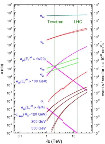
The g g fusion is the dominating mechanism for the Higgs production at the LHC over the whole Higgs mass spectrum, because of the high luminosity of gluons at the nominal centre of mass energy. The parton(in particular gluon) luminosity, is a convenient measure of the reach of a collider of given energy taking into account relevant Parton Distribution Function (PDF). The high gluon luminosity in pp collisions at LHC energies compared to Tevatron, is the basis for the simplifying slogan—“The Tevatron is a quark collider and the LHC is a gluon collider”. The g g fusion process is shown in Fig. 2.1(a), with a t -quark loop as the main contribution. Next-to-leading order QCD corrections have been found to increase the cross-section for this process by a factor of ∼ 2. Next-to-next-to leading order calculations are also available and show a further increase of about 10% to 30%. Other sources of uncertainty are the higher order corrections (10 ÷ 20% estimated) and the choice of parton density function (∼ 10%).
2.1.2 Vector Boson Fusion
The Vector boson fusion (VBF) (or VV fusion) shown in Fig. 2.1(b) is the second contribution to Higgs production cross section. It is about one order of magnitude lower than g g fusion for
2.1. Higgs Production [GeV] H M 100 200 300 400 500 1000 H+X) [pb] → (pp σ -2 10 -1 10 1 10 = 7 TeV s LHC HIGGS XS WG 2010
H (NNLO+NNLL QCD + NLO EW) →
pp
qqH (NNLO QCD + NLO EW) →
pp
WH (NNLO QCD + NLO EW) →
pp
ZH (NNLO QCD +NLO EW) → pp ttH (NLO QCD) → pp (a) [GeV] H M 80 100 200 300 400 1000 H+X) [pb] → (pp σ -2 10 -1 10 1 10 2 10 = 8 TeV s LHC HIGGS XS WG 2012
H (NNLO+NNLL QCD + NLO EW)
→
pp
qqH (NNLO QCD + NLO EW)
→
pp
WH (NNLO QCD + NLO EW)
→
pp
ZH (NNLO QCD +NLO EW)
→ pp ttH (NLO QCD) → pp (b)
Figure 2.2: Higgs production cross-sections at 7 and 8 TeV as a function of the Higgs mass.
a large range of mHvalues and the two processes become comparable only for very high Higgs
masses, of O (1 TeV). However, this channel is very interesting because of its clear experimental signature: the presence of two spectator jets with high invariant mass in the forward region provides a powerful tool to tag the signal events and discriminate the backgrounds, thus improving the signal to background ratio, despite the low cross-section. Moreover, both leading order and next-to-leading order cross-sections for this process are known with small uncertainties and the higher order QCD corrections are quite small.
2.1.3 Higgsstrahlung and Associated Production
In the Higgsstrahlung process shown in Fig. 2.1(c), the Higgs boson is produced in association with a W±or Z boson, which can be used to tag the event. The cross-section for this process is
several orders of magnitude lower than the g g fusion process, and approaches the production rates from VBF only for masses aroundmH= 100 GeV. The QCD corrections are quite large for
the Higgsstrahlung production modes. The next-to-leading order cross-section is found to be about 1.2–1.4 times larger than the leading-order one.
"The cross-section for this process [...] the gg fusion process, and approaches the production rates from VBF only for masses around [...]
The last process, illustrated in Fig. 2.1(d), is the associated production of a Higgs boson with a
t ¯t pair. Again the cross-section for this process is almost two orders of magnitude lower than
the g g and only several times lower than VBF around mH= 100 GeV. The presence of the t ¯t
pair in the final state can provide a good experimental signature. The higher order corrections increase the cross-section by a factor of about 1.2.
2.2 Higgs Decay
The branching ratios of the different Higgs decay channels are shown in Fig. 2.3 as a function of the Higgs mass. Fermion decay modes dominate the branching ratio in the low mass region (up to ∼ 150 GeV). In particular, the H → b ¯b channel is the most important contribution, since the b quark is the heaviest available fermion. When the decay channels into vector boson pairs open up, they quickly dominate. A peak in the H → W+W−decay is visible around 160 GeV, when the production of two on-shell W ’s becomes possible and the production of a real
Z Z pair is still not allowed. At high masses (∼ 350 GeV), also t ¯t pairs can be produced.
(a) (b)
Figure 2.3: Branching ratios for different Higgs decay channels as a function of the Higgs mass in low
mass range (a) and full search range (b).
The most promising decay channels for the Higgs discovery do not only depend on the corre-sponding branching ratios, but also on the capability of experimentally detecting the signal while rejecting the backgrounds. Such channels are illustrated in the following, depending on