HAL Id: tel-01620461
https://tel.archives-ouvertes.fr/tel-01620461
Submitted on 20 Oct 2017
HAL is a multi-disciplinary open access
archive for the deposit and dissemination of
sci-entific research documents, whether they are
pub-lished or not. The documents may come from
teaching and research institutions in France or
abroad, or from public or private research centers.
L’archive ouverte pluridisciplinaire HAL, est
destinée au dépôt et à la diffusion de documents
scientifiques de niveau recherche, publiés ou non,
émanant des établissements d’enseignement et de
recherche français ou étrangers, des laboratoires
publics ou privés.
To cite this version:
Walter Fuscaldo. Advanced radiating systems based on leaky waves and nondiffracting waves.
Elec-tronics. Université Rennes 1, 2017. English. �NNT : 2017REN1S015�. �tel-01620461�
THÈSE / UNIVERSITÉ DE RENNES 1
sous le sceau de l’Université Bretagne Loire
En Cotutelle Internationale avec
Università degli studi di Roma ‘Sapienza’
pour le grade de
DOCTEUR DE L’UNIVERSITÉ DE RENNES 1
Mention :
Électronique
Ecole doctorale Matisse
présentée par
Walter Fuscaldo
préparée à l’unité de recherche (UMR 6164 IETR)
(Institut d’
Électronique et de Télécommunications de Rennes)
(Composante universitaire)
Advanced Radiating
Systems based on
Leaky Waves and
Nondiffracting Waves
Thèse soutenue à Rome
le 27/02/2017
devant le jury composé de :
Mauro ETTORRE
Research Scientist CNRS, Université de Rennes 1/ directeur de thèse à Rennes
Alessandro GALLI
Professeur Université de Rome ‘Sapienza’ /
directeur de thèse à Rome
Franciso MEDINA-MENA
Professeur Université de Sevilla / rapporteur
Alessandro TOSCANO
Professeur Université de Rome Tre / rapporteur
Giuseppe SCHETTINI
Abstract xxxiii
Acknowledgments xxxv
Introduction xlv
i reconfigurable leaky-wave antennas for thz far-field
applications 1
1 conventional leaky-wave antennas 3
1.1 Introduction 3
1.2 Leaky-Wave Theory 5
1.2.1 Nature of waves 5
1.2.2 Physical significance of leaky waves 6
1.2.3 Mathematical significance of leaky waves 8
1.2.4 The transverse resonance technique 13
1.2.5 Classification of leaky-wave antennas 17
1.3 1-D Leaky-Wave Antennas 20
1.3.1 Historical examples of 1-D LWAS 20
1.3.2 Radiating properties of 1-D unidirectional
LWAs 22
1.3.3 Radiating properties of 1-D bidirectional LWAs 24
1.4 2-D Leaky-Wave Antennas 27
1.4.1 Historical examples of 2-D LWAS 27
1.4.2 Radiating properties of 2-D LWAs 28
1.4.3 Design rules for dielectric-based 2-D LWAs 30
1.4.4 Motivation for the study of unconventional 2-D
LWAs 31
1.5 Conclusion 33
2 formulas for leaky-wave antennas 35
2.1 Introduction 35
2.2 Formulas for 1-D Unidirectional Leaky-Wave Anten-nas 37
2.2.1 Analytical framework 37
2.2.2 Fitting procedure 40
2.2.3 Numerical results 44
2.2.4 Comparison with Oliner’s formula 49
2.2.5 Beamwidth evaluation at endfire 53
2.3 Formulas for 1-D Endfire Leaky-Wave Antennas 55
2.3.1 The modified Hansen-Woodyard condition for 1-D
LWAs 55
into account the∆θhvs. SLL tradeoff 63
2.3.5 Approximate formulas for the beamwidth and the sidelobe level 64
2.3.6 Investigation for extremely-efficient endfire leaky-wave antennas 67
2.4 Formulas for 1-D Bidirectional Leaky-Wave Antennas 71
2.4.1 Beamwidth formulas for uniform and infinite aper-tures 71
2.4.2 Beamwidth formulas for finite apertures 75
2.5 Conclusion 82
3 reconfigurable leaky-wave antennas 83
3.1 Introduction 83
3.2 Graphene-based Leaky-Wave Antennas 85
3.2.1 Graphene properties 87
3.2.2 Graphene plasmonics 93
3.2.3 Graphene planar waveguide 97
3.2.4 Graphene substrate-superstrate antenna 107
3.2.5 Graphene strip grating antennas 119
3.2.6 Technological aspects 122
3.3 Fabry-Perot Cavities Based on Liquid Crystals 125
3.3.1 Introduction 125
3.3.2 Liquid crystals 126
3.3.3 Electromagnetic model for nematic liquid crys-tals 127
3.3.4 Tunable THz Fabry-Perot cavity leaky-wave antenna based on NLCs 131
3.4 Conclusion 140
ii generation of nondiffracting beams and pulses for
near-field applications at millimeter waves 141
4 nondiffracting waves 143
4.1 Introduction 143
4.2 Mathematical framework 145
4.3 Bessel Beams 152
4.3.1 History, definition and properties 152
4.3.2 Potential applications 154
4.3.3 Realizations 155
4.4 X-Waves 158
4.4.1 History, definition and properties 158
4.4.3 Realizations 161
4.5 Conclusion 164
5 bessel-beam launchers 165
5.1 Introduction 165
5.2 Microwave Bessel-Beam Launchers 166
5.2.1 Theoretical analysis 166
5.2.2 Numerical results 171
5.2.3 Experimental results 173
5.2.4 Millimeter-wave design 175
5.3 Millimeter-wave Bessel-Beam Launchers 178
5.3.1 Design of the structure 179
5.3.2 Numerical validation 186
5.3.3 Prototype 189
5.3.4 Measurements 190
5.3.5 Use of a LRW as an X-wave launcher 194
5.4 Conclusion 196
6 x-wave launchers 197
6.1 Introduction 197
6.2 Zeroth-Order X-Wave Generation Through Finite Aper-tures 198
6.2.1 Metric of confinement 199
6.2.2 Ideal X-waves 201
6.2.3 Dispersive X-waves 209
6.2.4 Dispersive-finite X-waves 212
6.3 Higher-Order X-Wave Generation Through Finite Aper-tures 220
6.3.1 Analytical framework 221
6.3.2 Monochromatic higher-order Bessel beams 222
6.3.3 Polychromatic superposition of higher-order Bessel beams 223
6.3.4 Numerical results 225
6.4 Conclusion 227
a a possible proof about the definition of the pointing an-gle in lwas 229
b simulation model for the full-wave analysis of graphene-based lwas 231
bibliography 233
List of Publications 257
conductor (PEC/PMC) walls.
Figure 1.2 Ray intepretation of the physical significance of (a) a forward and (b) a backward leaky wave in a waveg-uiding structure of finite extent. Within a wedge-shaped region (highlighted in light blue) limited by the shadow boundary, the leaky-wave field domi-nates the near-field region. It is worth noting the ca-pability of backward leaky waves to focus radiation in the near field. 7
Figure 1.3 Classification of forward waves in open regions with respect to their propagating features. When αz =0 two kinds of waves exist: uniform plane waves
αx=0, and surface waves αx 6= 0. Surface waves might be proper of improper, depending on the sign of αx. When αz 6= 0, physical leaky waves exist only when αz > 0. Even more interestingly, in order to describe a radiation mechanism βx > 0, a forward leaky wave must be improper. 8
Figure 1.4 (a) Real <{ˆkz}part and (b) imaginary={ˆkz}part of ˆkz vs. f for a SW mode (black solid line) evolving in a LW mode (dotted green line), after ‘crossing’ the spectral gap (improper real SW are there repre-sented with green and black dashed lines) in a typ-ical GDS covered with a PRS. The nonphystyp-ical LW solution (which is the complex conjugate of the po-tentially physical one) is represented in dotted black line. 9
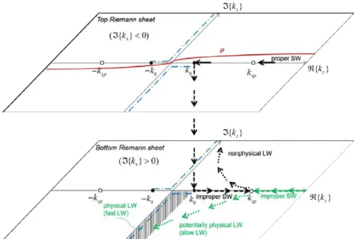
Figure 1.5 The top and bottom sheets (i.e., kz-planes) of the two-sheeted Riemann surface for kx. The Sommerfeld branch cuts are represented in blue dashed-dotted lines. Color styles and line styles are the same of Fig.1.4. The arrow indicates the direction for which
the frequency is decreasing. A path of integration, la-beled as P, is also shown in red solid line on the top Riemann sheet. 10
Figure 1.6 The deformation of the path P into P (solid red lines). The LW poles are represented with dotted cir-cles since they lie on the bottom Riemann sheet and thus they are not captured during the path deforma-tion. 11
Figure 1.7 Steepest descent φ-plane. The eight quadrants (from T1 to T4 for the top sheet and from B1 to B4 for the bottom sheet) constituting the two sheets are mapped in a single strip onto the φ-plane. The original path P (red solid line) is deformed into the SDP (black solid line) for any angle of observation θ. The extreme SDPs (ESDPs) are obtained for θ= ±π/2, and are reported
in black and white dashed line for the positive one (ESDP+) and the negative one (ESDP-), respectively. Only the poles which lie within ESDP+ and ESDP -may contribute to the radiated field. 13
Figure 1.8 2-D section and TEN model of (a) a PPW and (b) a GDS. 14
Figure 1.9 Dispersion diagram ˆkz vs. f of a PPW. Dispersion curves are found for εr = 1 and h = λ0/2 where
λ0 = 300 µm. Evanescent modes kz = −jαz in dashed lines and guided modes kz=βz∈R in solid lines. Since the structure is not simply-connected, a TEM mode (black solid line) propagating from DC frequency is obtained for m = 0 (green lines are for m=1 and blue lines are for m=2, TE-TM modes, re-spectively). Yellow dots indicates the cutoff frequen-cies fc(m). 15
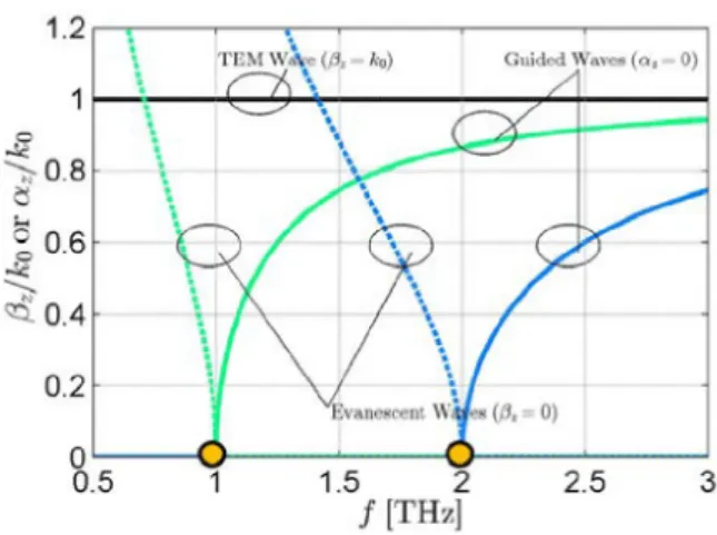
Figure 1.10 Dispersion diagram ˆkz vs. f of a GDS. Dispersion curves are found for εr = 2.17 and h= λ0/2 where
λ0 = 300µm. The light line kz = k0 sets the bound-ary between the radiating region (just below, high-lighted in blue) where leaky waves ( ˆβz in dashed blue lines and ˆαz in dotted blue lines) may describe radi-ation, and propagating region (just above, highlighted in green) where surface waves ( ˆβz in solid blue lines) may describe surface propagation. 16
Figure 1.11 Two well-known examples of 1-D LWAs. (a) An ex-ample of 1-D uniform LWA: the slitted rectangular waveguide [24]. (b) An example of 1-D quasi-uniform
LWA: the holey waveguide [25]. 20
Figure 1.12 Comparison between the far-field distributions of a uniform aperture distribution and a leaky aperture distribution. The directivity of LWAs increases as long as the leakage rate αzis low. 21
ture to avoid back-reflection from the forward leaky wave. 22
Figure 1.14 2-D section of a bidirectional LWA centrally-fed by a coaxial cable. When the two beams approaches each other, they merge in a single beam which points ex-actly at broadside. 24
Figure 1.15 The original ray explanation proposed by von Tren-tini in [49] for FPC-like antennas. At that time,
these kind of antennas were not recognized as 2-D LWAs. 28
Figure 1.16 Several examples of different types of PRS. The PRS consists of a single (a) dielectric layer, (b) a multistack of alternating dielectric layers, (c) a 2-D periodic ar-ray of metallic patches, and (d) its complementary version, i.e., slots in a thin metal plate. 29
Figure 2.1 thvs. a calculated numerically (black solid lines). The behavior of thhas been reported for (a) 0≤a≤1, (b) 0 ≤ a ≤ 3, (c) 0 ≤ a ≤ 10, and (d) 0 ≤ a ≤ 30. In (b) th has been fit with a cubic spline curve (blue circles). 40
Figure 2.2 Evolution of the third-order polynomial coeffients of the spline interpolation. 41
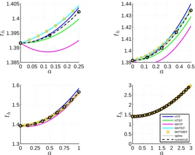
Figure 2.3 Comparison of data fitting of thvs. a by means of dif-ferent fitting functions in the range 0≤a≤0.25 (top-left corner), 0≤a≤0.5 (top-right corner), 0≤a≤1 (bottom-right corner), and 0≤a≤3 (bottom-left cor-ner). 43
Figure 2.4 (a) Asymptotic behavior of th vs. a for the various fitting functions in the range 0 ≤ a ≤ 3. (b) Abso-lute percent error (APE) vs. a of the various fitting functions in the range 0≤a≤3. 43
Figure 2.5 ∆θh vs. er for θ0 = 5◦, 15◦, 45◦, 90◦ (in order in red, yellow, green, blue) Comparison between aBW (in solid lines) and eBW (in circles) results for the evaluation of ∆θh for L=10λ (top-left corner), L=20λ (top-right corner), L=2λ (bottom-left cor-ner), L=100λ (bottom-right corner). 45
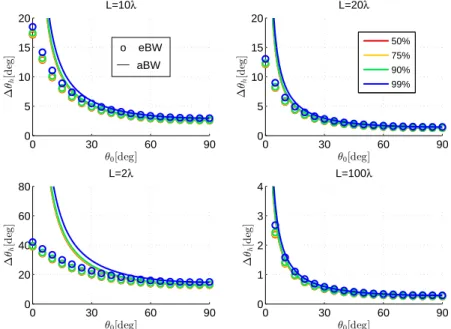
Figure 2.6 ∆θh vs. θ0 for er = 50%, 75%, 90%, 99% (in order in red, yellow, green, blue). Comparison between aBW (in solid lines) and eBW (in circles) results for the evaluation of ∆θh for L=10λ (top-left corner), L=20λ (top-right corner), L=2λ (bottom-left cor-ner), L=100λ (bottom-right corner). 46
Figure 2.7 APE (calculated as 100· |aBW−eBW|/|eBW|) vs. er for θ0 = 5◦, 15◦, 45◦, 90◦ (in order in red, yellow, green, blue) for L=10λ (top-left corner), L=20λ (top-right corner), L=2λ (bottom-left cor-ner), L=100λ (bottom-right corner). 46
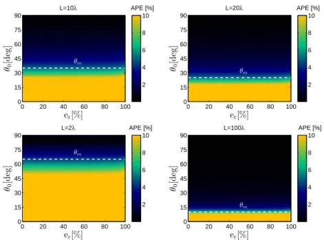
Figure 2.8 APE vs. θ0for er =50%, 75%, 90%, 99% (in order in red, yellow, green, blue) for L=10λ (top-left corner), L = 20λ (top-right corner), L= 2λ (bottom-left cor-ner), L=100λ (bottom-right corner). In black dashed lines the location of θmdefined as the minimum θ0for which the APE is less than 5%. 47
Figure 2.9 APE (calculated as 100· |aBW−eBW|/|eBW|) vs. θ0 and er. White dashed lines highlight the boundaries set by θm. 47
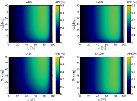
Figure 2.10 (a) APE (calculated as 100· |eFiBW−eBW|/|eBW|) vs. θ0 for er = 50%, 75%, 90%, 99% (in order in red, yellow, green, blue) and (b) APE vs. er for
θ0 =5◦, 15◦, 45◦, 90◦(in order in red, yellow, green, blue). The eFiBW is calculated using either the F1 (solid lines) or the F2 (dashed lines) formulas. Re-sults are shown only for L=10λ. 48
Figure 2.11 APE (calculated as 100· |eBW−eF1BW|/|eBW|) vs.
θ0and er. 49
Figure 2.12 P¯(θ) vs. θ (in linear scale) for different values of θ0 and er. 50
Figure 2.13 P¯(θ) vs. θ (in linear scale) for different values of θ0 when er = 90%. Lighter colored region represent the estimation of the single-sided beamwidth when using Oliner’s formula. The red solid line is reported for helping the reader to find the half-power value value. 51
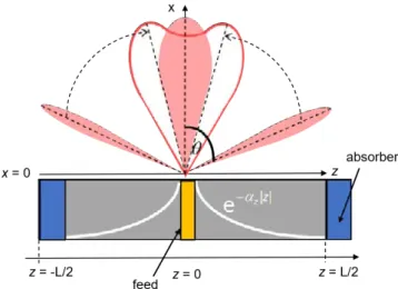
Figure 2.14 An example of a 1-D LWA. A leaky mode is excited at the source location z = 0. The metallic top wall of a rectangular waveguide is replaced by a partially reflecting screen to allow the propagating mode to leak out along the z-axis. The antenna is terminated with a matched load at z=L. 56
reaches the same intensity of the main lobe. 59
Figure 2.16 P¯(θ) vs. θ (in dB scale) for er ∈
{0%, 50%, 75%, 90%, 95%, 99%}, l = 10π, b = l (solid blue line) and b = l+∆bmax (dashed grey line), respectively. 60
Figure 2.17 (a) ¯P(θ) vs. θ for er =85.8%, l =20π, when∆b =0 (blue line) and ∆b = 1.47 (green line). (b) Fig. 4 of Reference [45] reported here for convenience. Case 1
and Case 2 perfectly match the blue and green curves, respectively. 61
Figure 2.18 P¯(θ) vs. θ for er ∈ {0%, 75%, 90%, 95%}, l = 10π, ∆b = 0 (red line), ∆b = 0.8 (green line), ∆b = 1.6 (blue line), and ∆b = 2.4 (black line) respectively.
62
Figure 2.19 ∆θh and SLL vs. b for er ∈
{0%, 50%, 75%, 90%, 95%}, L=10λ. 63
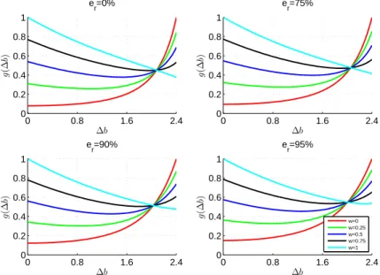
Figure 2.20 The optimizing function vs. ∆b for er ∈ {0%, 75%, 90%, 95%, 99%}, and for w=0, 0.25, 0.5, 0.75, 1 when L = 10λ. Obvi-ously, the extreme cases w = 0 and w = 1 would lead to the same b which minimizes the beamwidth and the SLL, respectively. 64
Figure 2.21 ∆θhand SLL vs. ∆b for er=0%, 75%, 90%, 95%. The magenta dot indicates the value of ∆b for which the SLL improves as er increases. 65
Figure 2.22 (a)∆θhand (b) SLL vs.∆b in the range 0≤∆b≤2.4. A family of a-parametric curves (solid lines) shading from blue to red is generated for a going from 0 to 0.8. Fitting curves are reported in circles in both figures.
66
Figure 2.23 (a) vi and (b) wi vs a for i = 0, 1, 2 (in order blue, green, and red solid lines) and their linear interpola-tions (dashed lines). 66
Figure 2.24 P¯(θ) vs. θ (in dB scale) for L = 10λ for er ∈
{99%, 99.5%, 99.9%, 99.95%, 99.99%, 100%}, b = l (blue line) and b=l+∆bmax(grey line), respectively. A blue dot highlights the location of the first sidelobe encountered from the main lobe for b=l. 67
Figure 2.25 P¯(θ) vs. θ (in dB scale) for (a) L = 1λ, (b)
L = 5λ, (c) L = 100λ, (d) L = 1000λ for er ∈
{99%, 99.5%, 99.95%, 100%}, b = l (blue line) and b = l+∆bmax (grey line), respectively. A blue dot highlights the location of the first sidelobe encoun-tered from the main lobe for b=l. 68
Figure 2.26 (a) th vs. a. A family of curves shading from blue to red is generated for r going from 0 to 1. The black solid line represent the result obtained through Eq. (2.12). (b) th vs. r. A family of curves shading
from blue to red are generated for a going from 0 to 10. 76
Figure 2.27 (a) th vs. a. A family of curves (solid lines) shading from blue to red is generated for r going from 0 to 1. The fitting curves are reported in circles. (b) w1vs. r (blue solid line) and w2vs. r (green solid line). The corresponding interpolations are reported in dashed lines. 77
Figure 2.28 thvs. a. A family of curves (solid lines) shading from blue to red is generated for r going from 0 to 1. The fitting curves are reported in circles. 78
Figure 2.29 Contour plot of APE vs. a and r. Left panel: APE is calculated after the first fitting procedure (see Fig. 2.27). Right panel: APE is calculated after the
second (last) fitting procedure (see Fig.2.28). 78
Figure 2.30 (a) th vs. a. A family of curves (solid lines) shading from blue to red is generated for r going from 0 to 1. The fitting curves are reported in circles. (b) w1vs. r (blue solid line), w2 vs. r (green solid line), and w3 (red solid line). The corresponding interpolations are reported in dashed lines. 79
Figure 2.31 thvs. a. A family of curves (solid lines) shading from blue to red is generated for r going from 0 to 1. The fitting curves are reported in circles. 80
Figure 2.32 Contour plot of APE vs. a and r. Left panel: APE is calculated after the first fitting procedure (see Fig. 2.30). Right panel: APE is calculated after the
conical shape (linear dispersion) of the diagram in proximity of the K points of the firs Brillouin zone of graphene. Around the K points the Fermi velocity. The figure is a concession of [91]. 87
Figure 3.2 E0vs. µc in the range 0≤ µc ≤1 eV, obtained from
3.8, for εr =1 (air). 89
Figure 3.3 Real part (in red) and imaginary part (in blue) of the graphene surface conductivity as a function of the frequency. Comparison between the expressions of the non-local model, i.e., σρ (circles) and σφ (in
squares), and the Kubo formula σ (solid line). Re-sults are shown for µc = 0 eV and (a) kρ = k0, (b)
kρ=200k0. 90
Figure 3.4 Comparison between σ = σintra+σinter (solid lines) and σintra (dashed lines) in the low THz range 0.3≤ f ≤3 THz for µc = 0.1 eV and τ = 3 ps. The agreement remains good for reasonable values of µc and τ. 91
Figure 3.5 (a) Graphene surface conductivity vs. chemical po-tential in the range−1 to 1 eV at the frequency for fre-quency raising from 0.3 THz to 3 THz (colors shade from blue to cyan for σJ and from red to yellow for
σR, respectively). (b) Graphene surface conductivity vs. frequency in the band 0.3-3 THz for chemical po-tential raising from 0 to 1 eV (colors shade from blue to cyan for σJ and from red to yellow for σR, respec-tively). 92
Figure 3.6 (a) Graphene Re[σ] and Im[σ] vs. τ at f = 1 THz
for µc ranging from 0 eV to 1 eV. Re[σ] and Im[σ]
curves gradually shade from red to blue and from gray to black, respectively, as µcincreases from 0 eV to 1 eV. 92
Figure 3.7 Intensity of plasmonic dissipation losses ˆαSPP in the range [0, 1] in the σ complex plane. The dynamic range of ˆαSPP has been saturated to values greater than 1 for readability purposes. The paths followed by the graphene surface conductivity in the com-plex plane have been reported for values of f rang-ing from 0.75 THz to 1.25 THz (size of the symbols increases), τ ranging from 0.1 ps to 3 ps (symbols change shape in the following order: ◦,×,O,∗) and
µc ranging from 0.25 eV to 1 eV (color of the symbol change in the following order: red, green, blue, and yellow). The black region represents the area char-acterized by the highest dissipation losses and is at-tained by graphene samples with both lower µc and
τ. 94
Figure 3.8 SPP figures of merit: (a) M2 = (ˆβSPP−1)/ ˆαSPP and (b) M3 = ˆβSPP/(2π ˆαSPP) vs. σR and σJ in the dynamic range shown in Fig. 3.5(a). The former
(Fig. 3.8(a)) gives a measure of the confinement of
a suspended SPP for 1-D and 2-D waveguide struc-tures. The latter (Fig. 3.8(b)) is strictly connected to
the quality factor Q [149]. 96
Figure 3.9 (a) 2-D sketch of the GPW structure (εr1 = 3.8). The biasing scheme is not reported. (b) Normalized field configurations of the tangential component of the electric field Ezat f =0.92 THz for the fundamental TM leaky mode (red line) and the SPP (blue line) in a GPW antenna. Grey and white regions represent the substrate and the air, respectively, whereas the black diamonds stand for the graphene sheeet. The x-axis is normalized to the height of the substrate h1. 97
Figure 3.10 2-D sketch, TEN model, and ABCD-matrix represen-tation of a GPW antenna. 98
Figure 3.11 Dispersion curves of SWs and LWs within the band 0.25−2 THz for a GDS (blue lines), a GPW (red lines), a BGPW (green lines), and a PPW (gray lines). In dashed lines improper waves, in solid lines proper waves. In (a) ˆβz, in (b) ˆαzfor TE modes, and in (c) ˆβz, in (d) ˆαz for TM modes. 99
mode and in solid blue line the remaining SWs. In (a) ˆβz, in (b) ˆαzfor TE modes, and in (c) ˆβz, in (d) ˆαz for TM modes. 100
Figure 3.13 Dispersion curves of the TE1, TM2fundamental LWs (a) within the band 0.75−1.1 THz for µc=0.5, 0.75, 1 eV, and (b) within the range 0.2 ≤ µc ≤ 1 eV for f = 0.92 THz. In (a) ˆβz and ˆαz are both represented in dashed lines for the TE1 mode and in solid lines for the TM2. In (b) ˆβz and ˆαz are represented in solid lines and dashed lines, respectively, for both modes. 101
Figure 3.14 Dispersion curves of (a) ˆβz, (b) ˆαz for the plasmonic mode SPP. Lines become brighter (red to yellow, and blue to cyan) as µcincreases from 0 to 1 eV. Note that as µcapproaches 1 eV the SPP mode approaches the PPW TEM mode. 102
Figure 3.15 (a) 2-D section of the structure and its transverse equivalent networks: (b) using the lossless model, (c) using the approximate Leontovich boundary con-dition, and (d) using the transition boundary condi-tion. 103
Figure 3.16 Effects of the introduction of losses and spatial dis-persion in the curves of the fundamental LWs in the band 0.9−0.95 THz for (a) TE and (b) TM modes. The red and green-blue lines consider the effect of dielectric losses and ohmic losses, respectively. The yellow ones consider the effect of a spatially dis-persive model in addition to dielectric and ohmic losses. 103
Figure 3.17 (a) Illustrative example of the typical scannable coni-cal beam-scanning feature of a GPW antenna. In (b) and (c), the radiation patterns normalized to the over-all maximum (achieved at broadside) vs. elevation angle θ for the GPW antenna represented in (a), are reported for the H-plane and E-plane, respectively. Analytical results are plotted in black solid lines, whereas full-wave results obtained with the tool CST Microwave Studio [159] are given by blue circles. The
scanning behavior at a fixed frequency ( fc = 0.922) is shown for beam maxima at θp = 0◦, 15◦, 30◦, 45◦. The corresponding chemical potentials are reported in the legend. 104
Figure 3.18 2-D sketch, TEN model, and ABCD-matrix represen-tation of a GSS antenna. 107
Figure 3.19 (a) The dispersion curve ( ˆβz and ˆαz vs. f in black solid and dashed lines, respectively) of the funda-mental TM leaky mode of the unperturbed SS is re-ported in the frequency range 0.75 ≤ f ≤1.25 THz. On the same plot the values of the splitting condi-tion ( ˆβz= ˆαz) are shown for different positions of the graphene sheet starting from the interface x0/h1=1 to the ground plane x0/h1=0. The color of the dots shades from red to blue as the graphene sheet moves from x0/h1 =1 to x0/h1= 0. An optimum position is found at f = 1.132 THz for x0/h1 = 0.82 (black dot). Note that the frequency fc at which splitting condition occurs ranges approximately from 1 THz to 1.5 THz. (b) Cutoff frequency fc (blue solid line) and relevant value of ˆβz(fc) = ˆαz(fc) (red dashed line) as a function of the normalized distance x0/h1 of the graphene sheet from the ground plane, for the fundamental TM mode in the GSS structure. 109
for x0/h1 = 0.805 (black dot). Note that the fre-quency fc at which splitting condition occurs ranges approximately from 1 THz to 1.5 THz. (b) Cut-off frequency fc (blue solid line) and relevant value of ˆβz(fc) = ˆαz(fc) (red dashed line) as a function of the normalized distance x0/h1 of the graphene sheet from the ground plane, for the fundamental TM mode in the GSS structure. 110
Figure 3.21 Cutoff frequency fc (blue to cyan solid lines) and relevant value of ˆβz(fc) = ˆαz(fc) (red to yellow solid lines) as a function of the distance of the graphene sheet from the ground plane x0 normal-ized to the substrate thickness h1, for the funda-mental TM leaky mode in the GSS. Similar results are found for the fundamental TE leaky mode. As the dielectric contrast spans the following values d1,2=2, 5, 10, 20, 50, the curves shade from blue to cyan and from red to yellow for values of fc and of
ˆαz(fc), respectively. 110
Figure 3.22 Normalized phase constants and attenuation con-stants of the fundamental TM (in black) and TE (in grey) leaky modes of a GPW (dashed lines) with pa-rameters as in [114] (i.e., with graphene placed at
the interface between the air and a dielectric layer at a fixed frequency fc = 0.92 THz) and of the pro-posed GSS (solid lines) with parameters as in Fig.
3.19, with graphene placed at the optimum position
x0 = 0.82h1 at a fixed frequency fc = 1.132 THz, as a function of the chemical potential in the range 1>µc>0 eV. 112
Figure 3.23 (a) Illustrative example of the typical conical beam-scanning feature of a GSS antenna. In (b) and (c), the radiation patterns normalized to the overall max-imum (achieved at broadside) vs. elevation angle θ for the GSS antenna represented in (a), are reported for the H-plane and E-plane, respectively. Analytical results are plotted in black solid lines, whereas full-wave results obtained with the tool CST Microfull-wave Studio [159] are given by blue circles. The scanning
behavior at a fixed frequency ( fc = 1.132 THz) is shown for beam maxima at θ =0◦, 15◦, 30◦, 45◦. The corresponding chemical potentials are reported in the legend. 113
Figure 3.24 H-plane radiation patterns, normalized to the over-all maximum (achieved at broadside), vs. elevation angle θ for a GSS antenna (solid lines) with param-eters as in Fig. 3.22 and for an equivalent GPW
(dashed lines), excited by a HMD placed on the ground plane. The scanning behavior at a fixed fre-quency ( fc=1.132 THz for the GSS and fc = 0.92 THz for the GPW) is shown for four theoretical point-ing angles θp =sin−1(ˆβ2z−ˆαz2)1/2= 0◦, 15◦, 30◦, 45◦. The chemical potentials for the GPW and the GSS are reported in the legend. 114
Figure 3.25 (a) Efficiency η vs. graphene positions in the sub-strate x0/h1 (red lines), and directivity at broadside normalized to its maximum ¯D0 (blue lines). Both η and ¯D0 have been calculated at the corresponding cutoff frequency for each graphene position x0/h1. The grey dashed line, representing the efficiency of an equivalent GPW antenna, has been reported for comparison. (b) The function f vs. x0/h1of Eq. (3.38)
for different values of w. Color of the lines shades from blue to red as w ranges from 0 to 1. Colored dots highlight the positions of the maxima of f as w ranges from 0 (blue dot) to 1 (red dot). Maxima are located closer to the interface as the efficiency is weighted more than the directivity. 116
face x0=h1. Light grey, dark grey, and white regions represent the substrate, the superstrate, and the air, respectively, whereas the black diamonds stand for the graphene sheet. The x-axis is normalized to the height of the overall structure h=h1+h2. 117
Figure 3.27 2-D section of the GSG antenna and its TEN model. 120
Figure 3.28 Dispersion diagrams of ˆβz and ˆαz vs. f for (a)-(c) TE and (b)-(d) TM fundamental leaky modes of a (a)-(b) graphene-based planar single-slab antenna (solid lines) and a (c)-(d) graphene-strip grating antenna (dashed lines). The values of the chemical potentials
µcare reported in the legends. 121
Figure 3.29 Normalized radiation patterns P(θ)/Pmax vs. θ for (a) TE and (b) TM fundamental leaky mode of a GPW (blue lines) and a GSG (red lines). 122
Figure 3.30 Representation of NLC molecules twisting in a LC cell. The optical axis of the NLC switches under the effect of an applied bias voltage. 126
Figure 3.31 2-D section (a) on the xy-plane and (b) on the xz-plane of the THz fishnet MM. Further details on the unit-cell are available in [96]. 127
Figure 3.32 Real part of the diagonal terms εii(x, y, z = 0) vs. xy-plane of the relative permittivity tensor for Vbias=0−7[V]. First column (i = x), second col-umn (i=y), and third column (i=z). Starting from the first row the driving voltage takes the following values: {0, 1.5, 2, 3, 4, 7}[V]. 128
Figure 3.33 Real part of the off-diagonal terms εij(x, y, z = 0) vs. xy-plane of the relative permittivity tensor for Vbias= 0−7 [V]. First column (i=x, j =y), second column (i=y, j=z), and third column (i=x, j=z). Starting from the first row the driving voltage takes the following values: {0, 1.5, 2, 3, 4, 7}[V]. 129
Figure 3.34 Real part of the diagonal terms εii(x=x0, y=y0, z) vs. z for Vbias=0−7 [V]. First column (i = x), second column (i = y), and third column (i=z). Starting from the first row the(x0, y0)position takes the following values: (0, 0) µm, (54, 54) µm, and (75, 75)µm. 130
Figure 3.35 Imaginary part of the diagonal terms
εii(x =x0, y=y0, z) vs. z for Vbias=0−7 [V]. First column (i = x), second column (i = y), and third column (i=z). Starting from the first row the (x0, y0) position takes the following values:
(0, 0)µm,(54, 54)µm, and(75, 75)µm. 131
Figure 3.36 2-D section view of the proposed device and its equivalent transmission-line representation. The NLC layers are biased through a pair of extremely-thin moderately-conductive polymer films (not re-ported in the picture), e.g., PEDOT:PSS [99], whose
absorption is neglected here. 132
Figure 3.37 Dispersion curves ( ˆβzand ˆαzvs. f ) of the fundamen-tal TM leaky mode for (a) Layouts 1, (b) 2, (c) 3, and (d) 4 (see Table3.5) when the NLC layer is biased at
V∞(blue lines) and when is unbiased 0 V (red lines). Colors gradually shades from blue to red as Vb de-creases from V∞to 0 V. 134
Figure 3.38 Radiation patterns predicted considering only the LW pole contribution (dashed lines) and by means of reciprocity theorem (solid lines) for (a) Layouts 1, (b) 2, (c) 3, and (d) 4 (see Table 3.5) when the beam
points at broadside (blue lines) and when is steered at the maximum pointing angle (red lines). 136
Figure 3.39 Dispersion curves ( ˆβzand ˆαzvs. f ) of the fundamen-tal TM leaky mode for (a) Layout 2 and (b) Layout 4 (see Table3.5) in the lossy case, when the NLC layer
is biased at V∞(blue lines) and when is unbiased 0 V (red lines). Colors gradually shades from blue to red as Vbdecreases from V∞to 0 V. 137
Figure 3.40 Radiation patterns for (a) Layout 2 and (b) Layout 4 for radiation at broadside (solid) and at the maxi-mum pointing angle (dashed). The radiation patterns have been calculated by means of reciprocity theorem in both the lossless (in red) and the lossy (in black) case, and then compared with those given by means of LWA theory (blue). Full-wave simulations with CST are also reported for the lossy case for radiation at broadside (filled green circles) and at the maxi-mum pointing angle (empty green circles). 138
Figure 4.1 Wavevectors κ=kρˆρ0+kzˆz0lying on the surface of a
Figure 4.3 Intensity distribution of a zeroth-order Bessel func-tion of the first kind (black solid line) and its enve-lope (blue dashed line) decaying as ρ−1. 152
Figure 4.4 Contour-plot of a zeroth-order Bessel beam gener-ated by an (a) infinite aperture and (b) a finite aper-ture of radius radius ρap = 3λ and with an axicon angle θ0=45◦. 153
Figure 4.5 (a) A sketch of the experimental setup used by J. Durnin for the first generation of a Bessel beam in optics [188]. (b) A sketch of the experimental setup
for generation of a Bessel beam through an axicon lens as presented in [222]. The axicon element
al-lows for converting a Gaussian beam in a Bessel beam within a rhomboidal region located in the near field. The dashed red line is located at z = zndr/2. In the far-field, the Fourier-Transform of the aperture field gives rise to the expected annulus shape. 155
Figure 4.6 (a) 2-D and (b) 3-D plot of the normalized amplitude of an X-wave as a function of ρ and z−vzt where vz is the group velocity of the wave. Since for an ideal X-wave cone dispersion is neglected, the group velocity vz coincides with the phase velocity vph =c/ cos θ0. As a consequence the variable z−vzt gives a measure of the spatio-temporal confinement of the pulse. In this example, we have considered a wide uniform fre-quency spectrum and an axicon angle θ0=45◦. The X-shape of the pulse follows the inclination dictated by the axicon angle, as emphasized by the boundaries in both figures. 159
Figure 4.7 (a) A sketch of the experimental setup used by Lu and Greenleaf for the first generation of X-waves in acoustics [263]. (b) A sketch of the experimental
setup for the first measurement of the 3-D field dis-tribution of X-waves in optics [264]. Except for a
sys-tem of converging lenses and a pinhole, the mech-anism of generation was equal to the one originally proposed by Durnin [188] for the Bessel beam
Figure 5.1 Geometrical view of a leaky-wave radial waveguide of thickness h. A metallic rim is placed at ρ = ρap. The PRS is represented by a square lattice of metallic patches. 167
Figure 5.2 The mechanism of generation of a Bessel beam through the superposition of an inward Hankel wave and an outward Hankel wave. An outward Hankel wave is generated at the center by a coaxial feed and is then reflected back by the circular metallic rim to create an inward Hankel wave. If the circular rim is placed in one of the zeros of the Bessel function and the incident wave is slowly-attenuated, the two Hankel waves constructively interfere each other and create the Bessel beam. 168
Figure 5.3 (a) 2-D section of the LRW and its (b) transverse equivalent network (TEN) model. 170
Figure 5.4 βρ/k0 vs. frequency ( f ). The intersections
be-tween the transverse (solid blue lines) and the radial (black dashed lines) resonances define the operating points. 171
Figure 5.5 β(n)ρ /k0 vs. f . The intersections between the trans-verse (solid blue lines) and the radial (black dashed lines) resonances define the operating points of the launcher. The radial resonance are reported only for 4≤n≤6. 172
Figure 5.6 Contour plot of the electric field |Ez| along the ρz-plane for the proposed LRW at the operating fre-quency f = 10 GHz. The five nulls are clearly dis-tinguishable, as expected from theory. 173
Figure 5.7 Final prototype. The array of vias comprising the outer metallic rim is shown in the inset. Courtesy of Mauro Ettorre [234]. 173
Figure 5.8 Normalized component Ez of the electric field. (a) Comparison between measured and simulated re-sults at z = 0.75λ0 for different φ-cuts. (b) 2D field distribution over the xy-plane at f = 9.6 GHz at z=0.75λ0. (c) 2D field distribution over the xz-plane at f =9.6 GHz at y= 0. Courtesy of Mauro Ettorre [234]. 174
Figure 5.9 2-D section of a PPW with lossy metallic plates. 175
Figure 5.10 αc vs. frequency ( f ). At f = 40 GHz the at-tenuation constant of the TEM mode propagating in a PPW with copper plates reaches the value of 7 Np/m. 176
g = 200 µm to g = 50 µm, which is the maximum tolerance for PCB technology. 177
Figure 5.12 Illustration of the millimeter-wave Bessel-beam launcher under consideration. The blue arrows show the outward and inward Hankel waves excited by a central coaxial probe. The constructive interference of these cylindrical waves creates the Bessel beam pro-file. 179
Figure 5.13 (a) Normalized phase constant and (b) normalized attenuation constant vs. frequency f up to 100 GHz for the first three TM of a LRW as in Fig. 5.3. The
solid and dashed lines denote the dispersion curves for the proper and improper modes, respectively. The blue and red curves represent the dispersion curves for the real and complex modes, respectively. Hence surface-wave (SW) modes are shown by black solid lines, whereas the leaky-wave (LW) modes are shown by grey dashed lines. In these plots, it is assumed that Xs= −25Ω, εr =2.17, h=3.175 mm [153]. 183
Figure 5.14 Dispersion curves (SW and LW in blue solid and red dashed lines, respectively) for the design of the higher-order launcher prototype. The operating points are given by the intersections of the fast leaky-wave modes and the hyperbolic curves given by the Bessel zeros (black dashed lines). Once the operat-ing point is chosen, the operatoperat-ing bandwidth (high-lighted gray region) is fixed by the closest intersec-tions of either the fast leaky-wave or the surface-wave modes. The parameters used in Fig.5.13are also
as-sumed here. 184
Figure 5.15 Geometrical interpretation of the problem in Fig.5.14. The blue dot represents the operating point
given by the intersection between q = 5 and n = 1 dispersion curves. The green dots represent the oper-ating points given by the intersection between n=1, and q=4, 6 dispersion curves. Once a0 is found, it can be used to calculate both finfLW1 and fsupLW1, thanks to the symmetry of the problem. 185
Figure 5.16 Approximation of the tangent function tan(kz1h) vs. h with (kz1h−nπ) for n = 0, 1, 2 when kz1=k0
q
εr−ˆk2ρ with ˆkρ = 0.8. As expected, at
h=3.175 mm the approximation is very good, lead-ing to percentage error of 0.3%. 187
Figure 5.17 (a) Geometry of the COMSOL model of the proto-type. The size of the evaluation box is set slighlty larger than necessary in order to avoid spurious re-flections from the PML boundary conditions. (b) Boundary conditions setting of the COMSOL model of the prototype. 187
Figure 5.18 Contour plot of the electric field |Ez| along the ρz-plane for the mm-wave launcher under analysis at (a) f =39.7 GHz, (b) f =37.3 GHz, and (c) f =40.3 GHz. 188
Figure 5.19 1-D profile of the normalized electric field|Ez|at f = 39.7 GHz, for the proposed launcher (parameters as in Fig.5.13), for various distances z= λ/2, λ, 3λ/2,
2λ from the aperture. 188
Figure 5.20 Prototype of the mm-wave leaky-mode Bessel-beam launcher. The feeding probe can be recognized at the center of the structure. 189
Figure 5.21 Schematic of the coaxial probe transition used for matching the mm-wave launcher. 189
Figure 5.22 HFSS unit-cell model for the impedance synthesis of the capacitive sheet. The respect of the homogeniza-tion limit p λop [50] allows for describing the
fields with only the fundamental n =0 Floquet har-monic, and hence only an equivalent transmission-line is required to model the structure. 190
Figure 5.23 Some pictures of the Near-Field Test Range at IETR, Rennes, France. Courtesy of Ioannis Iliopoulos [285].
Note that the antenna under test (AUT) shown in the picture on the left is not our actual prototype which was not mounted on the mast. These pictures are reported just to show the measurement setup. 191
Figure 5.24 (a) Measured reflection coefficient (|S11| in dB) and (b) reflection phase (∠S11) of the prototype in the fre-quency range 37÷40GHz. The black dashed lines highlight the frequency range for which the return loss is under−10 dB. 191
Figure 5.25 Measured intensity of Ez along
the xy plane at f =38.3 GHz at
z=0.5λ0, 0.75λ0, λ0, 1.5λ0, 2λ0, 2.5λ0 from the impedance surface, where λ0equal to 7.5 mm. 192
lines), simulations (dashed blue lines), and numer-ical results (red dashed lines). (a)-(c) Normalized Ez vs. ρ at f = 38.3 GHz at z = 0.5λ0, 0.75λ0,
λ0. (d)-(f) Normalized Ez vs. ρ at z = λ at
f =38.0 GHz, 38.8 GHz, 39.5 GHz. 193
Figure 5.28 Measured intensity of Ez along the xz plane at f =38.0 GHz, 38.3 GHz, 38.6 GHz, 38.9 GHz, 39.2 GHz, 39.5 GHz. 193
Figure 5.29 Measured HPBW vs. f in the range 38 GHz to 39.5 GHz at different distances z=0.5λ0, 0.75λ0, λ0, 1.5λ0, 2λ0, 2.5λ0. The color shades from blue to cyan as z increases from 0.5 λ to 2.5 λ. At z = λ the HPBW shows a remarkable
stability with respect to the frequency. 194
Figure 6.1 Definition of a metric of confinement for an X-wave. A pulse characterized by a transverse spot width Sρ
and a longitudinal spot width Szis launched through a finite radiating aperture of diameter dap = 2ρap. Since the main constituents of an X-wave, i.e., Bessel beams, maintain their spot widths up to the non-diffractive range zndr, an X-wave will be properly defined over an area on the ρz plane which is lim-ited along ρ by the aperture diameter and along z by the nondiffractive range. If most of the energy of the pulse is contained in this region, we can ac-tually state that the considered X-wave is efficiently confined. 199
Figure 6.2 Normalized χU
t (ρ) vs. ρ for f0 = 60 GHz, θ0 = 11◦ and (a)∆ω/ω0=0.05 (b)∆ω/ω0=0.2. Comparison between the numerical integration of Eq. (6.12) (red
circles), the exact integral of Eq. (6.12) (green solid
curves), and the approximation given by Eq. (6.15)
(blue dashed curves). As the fractional bandwidth ∆ω/ω0 increases, the approximation is less accurate on the tails, but the width of the main beam is always well approximated. 203
Figure 6.3 Weak confinement Cρ,z vs. ρap/λ0 and θ. The
yel-low hyperbola represents the boundary between the region of efficient (in white) and non-efficient con-finement (in black) for ideal UXWs, when fractional bandwidths of (a) ∆ω = 0.01, (b) ∆ω = 0.05, (c) ∆ω = 0.1, and (d) ∆ω = 0.2 are considered. The region of efficient confinement increases for larger fractional bandwidths. In any case, this region corre-sponds to electrically large apertures with small axi-con angles. 205
Figure 6.4 The yellow and white hyperbola represents the boundaries between the region of efficient (in white) and non-efficient confinement (in black) ∆ω = 0.01 and ∆ω = 0.2, respectively. The transition region is limited by the two hyperbola. 206
Figure 6.5 Cρ(w),z vs. ρap/λ0 and θ0 for (a) FBW = 1% and (d) FBW = 20%. The purple dot p1 represents an X-wave with m = 8 and θ = 10◦. The yellow dot p2 represents an X-wave with m = 1 and θ = 10◦. The blue dot p3 represents an X-wave with m = 25 and θ = 20◦. An X-wave in p1 is generated for (b) FBW=1% and (c) FBW=20%, whereas X-waves in (e) p2and (f) p3are both generated for FBW=20%. In (b-c) and (e-f), the intensity of the X-wave is re-ported over a ρz plane limited by ρap along ρ and zndr along z. From this representation, if Sρ and Sz
fit in the plot, then the X-wave is confined over the respective axis. Note that, the ρ-axis is normalized to
ρapwhile the z-axis is normalized to zndr. 206
Figure 6.6 Strong confinement C(s)ρ,zvs. ρap/λ0and θ. The yellow
curves represent the boundaries between the region of efficient (in white) and non-efficient confinement (in black) for ideal UXWs, when fractional band-widths of (a)∆ω=0.01, (b)∆ω=0.05, (c)∆ω=0.1, and (d) ∆ω = 0.2 are considered. The region of efficient confinement increases for larger fractional bandwidths as for C(w)ρ,z . However, the efficient region is considerably narrower due to the more strict crite-rion applied by the strong metric C(s)ρ,z with respect to the weak metric C(w)ρ,z . 207
θ0=30◦for p2). 208
Figure 6.8 Comparison between numerical integrations (red cir-cles) and approximations (Eqs. (6.29) and (6.17) in
green solid lines and Eqs.6.18and6.19in blue dashed
lines) of (a)-(b) transverse profiles and (c)-(d) longi-tudinal profiles for a dispersive X-wave in fractional bandwidths (a)-(c) FBW = 5% and (b)-(d) FBW =
20% centered around f0 = 60 GHz. The result-ing profiles have been obtained assumresult-ing kz0=0.2k0, kz1=0.55·10−12, and kz2=0. Results are reported over an aperture plane of ρap = 15λ0 and zndr calculated at f0. Note that ρ0 = kρ0ρ and z0 =
kz0∆ωz/2. 211
Figure 6.9 (a) Prospective view of an RLSA. (b) Brillouin di-agram f vs. kz for the structure in Fig. 6.9. kz
(green curve) is given by Eq.6.33through the relation
of separability. The second-order Taylor approxima-tion (blue circles) accurately describe the wavenum-ber dispersion curve. The slope of kz is lower than the light line (black line), so that c0>vz>0. 212
Figure 6.10 2-D normalized intensities for ideal (first column: (a) and (d)), dispersive (second column: (b) and (e)), and dispersive-finite (third column: (c) and (f)) UXWs, when the pulse has reached half the propagating dis-tance of z(c)dof. The numerical results are shown for ∆ω = 0.05 (first row: (a-c)), and ∆ω = 0.2 (second row: (d-f)). 215
Figure 6.11 Evolution of the (a) transverse and (b) longitudinal HPBW vs. t. The ideal (red curves), dispersive (green curves), and the dispersive-finite case (blue curves) are represented for∆ω = 0.2. The x-axis on the top is obtained by scaling the temporal axis with the the-oretical group velocity vz'0.84c0. 216
Figure 6.12 Evolution of the normalized intensity vs. time t. The ideal (red solid line), dispersive (green dashed line), and the dispersive-finite case (blue circles) are repre-sented for∆ω=0.2. 217
bandwidth∆ω =0.2. The time evolution is numeri-cally reproduced for 9 different time frames, ordered from left to right and from top to bottom. 218
Figure 6.14 Schematic view of the generation of localized twisted pulses from a radiating aperture on the xy plane. The intersection of the shadow boundaries (dot-ted black lines) defines the nondiffractive range (zndr=ρapcot θ). Dashed red lines define the enve-lope of the confined region whose section slowly in-creases beyond the nondiffractive range due to the limited spatio-temporal dispersion of the pulse. In the numerical examples of6.3.4the transverse
distri-butions are observed at the reference plane for differ-ent time instants. 221
Figure 6.15 Normalized amplitude distribution of Ez vs. x, y at f =12.5 GHz with kρ = 0.4k0of the near field radi-ated over the transverse (i.e., xy) plane at z=zndr/2. (a-c) Contour plot of Ez radiated at z = zndr/2 by a standing-wave aperture distribution (Eqs. (6.40
)-(6.41)) and (d-f) by an inward traveling-wave aperture
distribution (Eqs. (6.42)-(6.43)) for n=1, 3, 5
(look-ing from left to right) over a radiat(look-ing aperture with radius ρap=10λ. 222
Figure 6.16 Phase distribution at f = 12.5 GHz with kρ = 0.4k0 of the Eznear field obtained by radiating a first-order inward traveling-wave distribution over the trans-verse (i.e., xy) plane at z = zndr/2. The correspon-dent normalized amplitude distribution is given in Fig.6.15(d). 223
Figure 6.17 Comparison between (a)-(b) nondispersive and (c)-(d) dispersive case. The norm of χEis reported over the xz plane. The x-axis is normalized to λ0, whereas the z-axis is normalized to z(c)ndr. The contour plot of
||χE||has been reported for two time instants: (a), (c) ti=0.8 ns and (b), (d) tf =2.4 ns. 225
Figure 6.18 Screen-shots of (a) χρ, (b) χφ, (c) χz, and (d)||χE||at t1= 0.8 ns, t2 = 1.3 ns over the xy plane (both axes are normalized to λ). Note that the colorscale for (d) and (h) is different since||χE|| >0. 226
tangential magnetic field Hy at the ground plane is represented with a blue arrow. (b) Phase-shift walls have been implemented to emulate an infinitely transverse uniform structure by means of a periodic unit cell. 231
L I S T O F T A B L E S
Table 2.1 MAPE for HTF, HETF, MHTF, MHTEF, MHTMEF and spline approximations. 42
Table 2.2 Values of the fitting parameters for HTF, HTEF, MHTF, MHTEF, and MHTMEF functions. 44
Table 2.3 Values of NO to have the exact beamwidhth evalua-tion. 50
Table 2.4 Evaluation of OBW, eBW and APE in the range 5◦≤θ0≤90◦ for er = 90% and antenna lengths L=10λ and L=20λ. 52
Table 2.5 Variation of NO in the range 5◦≤θ0≤90◦ and for er = 50%÷99.9994% antenna lengths L=102λ, 104λ, 106λ. 52
Table 2.6 Values of τ for different antenna efficiencies er. 57
Table 2.7 Values of ∆bmax for different antenna efficiencies er. 60
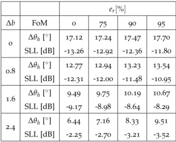
Table 2.8 Figures of Merit (FoM), namely∆θhand SLL, for dif-ferent values of ∆b and different antenna efficiencies er, for L=10λ. 62
Table 2.9 Fitting parameters for∆θhand SLL. 67
Table 2.10 Values of the fitting coefficients for w1(r) and w2(r). 77
Table 2.11 Values of the fitting coefficients for w1(r), w2(r)and w3(r). 79
Table 3.1 HPBW on H(E)-planes for different bias-scanned pointing angles of GSS and GPW antennas at fixed frequency. 115
Table 3.2 HPBW on both H(E)-planes for different frequency-scanned pointing angles of GSS, GPW (at fixed
µc=1 eV), and SS antennas. 116
Table 3.3 Comparison of efficiency η, directivity at broadside D0and reconfigurability∆θ (scanning angular range) for GPW and GSS antennas, for different quality (τ) of the graphene sheet. 118
Table 3.4 Comparison of directivity and reconfigurability for GSS antennas with different efficiencies and for dif-ferent quality (τ) of the graphene sheet. 119
Table 3.5 Relevant parameters for the design of the proposed THz FPC-LWAs based on NLC. 133
Table 3.6 Radiating performance in terms of beam reconfigura-bility (θMp), directivity (D0) and beamwidth (∆θ), for all layouts. 135
Table 3.7 Performance of Layout 2 and 4 in lossless and lossy case. 138
In recent years, microwave, millimeter-wave, and THz applications such as medical and security imaging, wireless power transfer, and near-field focusing, just to mention but a few, have gained much attention in the area of ICT due to their potentially high social impact. On one hand, the need of highly-directive THz sensors with tunable radiating features in the far-field region has recently boosted the research activity in the design of flexible, low-cost and low-profile devices. On the other hand, it is of paramount importance to focus energy in the near-field region, and thus the generation of limited-diffraction waves in the microwave and millimeter-wave regime is a topic of recent increasing interest.
In this context, leaky-wave theory is an elegant and extremely useful for-malism which allows for describing in a common fashion guiding and radi-ating phenomena in both the near field and the far field, spanning frequen-cies from microwaves to optics passing through THz.
In this PhD thesis we aim to exploit the intrinsic versatility of the leaky-wave approach to design advanced radiating systems for controlling the far-field radiating features at THz frequencies and for focusing electromag-netic radiation in the near field at millimeter waves. Specifically, the use of relatively new materials such as graphene and liquid crystals has been consid-ered for the design of leaky-wave based radiators, achieving very promis-ing results in terms of reconfigurability, efficiency, and radiatpromis-ing capabili-ties. In this context, an original theoretical analysis has provided new gen-eral formulas for the evaluation of the radiating features (e.g., half-power beamwidth, sidelobe level, etc.) of leaky-wave antennas. Indeed, the cur-rent formulations are based on several simplifying hypotheses which do not allow for an accurate evaluation of the beamwidth in different situations.
In addition to the intriguing reconfigurable capabilities offered by leaky waves in far-field applications, interesting focusing capabilities can be ob-tained in the near field. In particular, it is shown that leaky waves can profitably be used to generate limited-diffraction Bessel beams by means of narrow-band radiators in the microwave range. Also, the use of higher-order leaky-wave modes allows for achieving almost the same performance in the millimeter-wave range, where previous designs were subjected to severe fabrication issues. Even more interestingly, the limited-diffractive character of Bessel beams can also be used to generate limited-diffraction pulses as superpositions of monochromatic Bessel beams over a consider-able fractional bandwidth. In this context, a novel theoretical framework has been developed to understand the practical limitations to efficiently generate limited-diffraction, limited-dispersion pulses, such as X-waves, in
A C K N O W L E D G M E N T S
Three long years of PhD have passed since I have decided to dedicate my life to this wonderful path called scientific research. This experience has been alternately scattered by hard and nice moments. However, I cannot forget the wonderful people that I had the luck to meet along this path, and that have individually contributed to enrich either my knowledge with their experience, or my life with their presence.
This part of the PhD thesis is dedicated to them, so I can thank them all one by one (each one in their native language, to the best of my knowledge!): Grazie Guido Valerio. Sei la prima persona che ho incontrato nel mio cammino scientifico: dalla tesi di triennale (che forse ricordi a malapena!), a quella più significativa di magistrale, per poi proseguire nei primi anni di PhD. Sarebbe facile dire che avrei gradito collaborare ancor di più, ma preferisco ritenermi già immensamente fortunato per averti conosciuto nel momento più delicato della mia formazione scientifica. Grazie ancora e... Viva le analisi dispersive!.
Grazie Alessandro Galli. È particolarmente difficile condensare in poche parole quanto la sua presenza sia stata importante per fare di me lo studente di PhD che sono oggi. Dal primo giorno in cui rimasi ‘affascinato’ dai riferimenti artistici all’elettromagnetismo, a oggi in cui tra una ricerca e l’altra ci sfugge un commento al cinema, alla letteratura, all’arte in genere che tanto ci appassiona. Perché entrambi sappiamo che, per quanto sia grande la scienza, la vita è davvero piccola senza la magia dell’arte. Grazie ancora per aver illuminato questo mio cammino.
Grazie Mauro Ettorre. Sei stato la prima persona ‘di scienza’ che ho in-contrato fuori dall’Italia, nella mia prima esperienza all’estero. Ho sempre apprezzato la tua sincerità a fronte di qualche differenza di vedute. Alcune cose hanno funzionato altre meno, ma dal nostro confronto e dalla nostra collaborazione sono nati grandi cose. Non scorderò mai l’emozione nel vedere le misure del nostro lanciatore... Credo che ci siano poche cose che ripaghino il lavoro di un ricercatore più del vedere la conferma di una teoria da parte di un esperimento. Grazie.
Grazie Paolo Burghignoli. Per un ex-studente di Matematica, che si ram-marica tuttora di non aver avuto la forza di completare quel percorso, non poteva esserci miglior fortuna che incontrare te. Mi sono imbattuto in tanti ingegneri e matematici e posso dire che, per distacco, rappresenti il miglior
mi sono oggi così chiari grazie all’accuratezza delle tue spiegazioni. Grazie per avermi fatto fatto acquisire padronanza di certe tematiche.
Thank you David R. Jackson. After spending four months in Houston, I have understood the reason why Guido defined it human-unfriendly! It is even more true that I do not think it does exist in the world any other place where one can hope to learn something about leaky waves, because of you. Since the very first day I was really impressed by your intuition about physical phenomena. However, what I will really miss is our Running Wednesdays/Saturdays. Thank you for always treating me as a friend rather than as a student.
Grazie Germana Peggion. Quante probabilità ci sono di conoscere una ‘stravagante’ matematica/oceanografa in una base NATO a La Spezia? Non voglio saperlo, ma credo che la vita sia preziosa soprattutto perché ci regala questi eventi inaspettati. Avere guadagnato la tua amicizia prima ancora della tua stima è motivo di grande orgoglio per me. Grazie a te, ho ap-prezzato i ponti ‘non-euclidei’ di New Orleans (che sono paralleli ai fiumi), ammirato i quadri fatti con la sabbia di tua sorella Gabriella, visto la casa natale di uno dei miei scrittori preferiti (i.e., William Faulkner), e persino conosciuto il fantasma di casa tua. Insomma nella classifica dell’originalità vinci a mani basse! Grazie.
Grazie Caterina Dominijanni. Se oggi la mia sensibilità artistica, in partico-lare quella rivolta alla letteratura, si è sviluppata in un certo modo, lo devo in parte a Lei. Mi ha fatto conoscere dei paradisi letterari nei quali mi sono rifugiato e in cui continuo a rifugiarmi tuttora. Poche persone mi hanno saputo fare un regalo più bello. Grazie.
Grazie Costanza Parisella. A distanza di vent’anni resta la persona a cui mi sento più grato per quello che mi ha insegnato. La curiosità scientifica e la poetica sono le luci che lei ha acceso in me, e che tuttora svolgono il duplice compito di scaldare il mio cuore e al tempo stesso indicarmi la strada da percorrere. Grazie per aver acceso quelle luci.
Grazie Maurizio Fascetti. Se in questo laboratorio non ci siamo ancora abit-uati al tuo pensionamento, un motivo ci sarà! Ricordo sempre con piacere le lunghe chiacchierate sui massimi sistemi, così come custodisco gelosamente le perle di saggezza che parsimoniosamente hai dispensato. Grazie davvero.
Merci Noëlle Le Ber. Vous étiez pour moi, ma première enseignante de français, mon soutien spirituel dans mon séjour en France, et ma ‘mère’ d’adoption. Existe-t-il un moyen pour vous remercier pour tout ça? Je ne crois pas, mais j’éspère très fortement que la vie pourra un jour vous récompenser de votre gentilesse. Merci du fond du coeur.
Grazie Federica Polverari. Tra tutti i compagni di Dottorato, l’unica che mi sento di poter chiamare un’amica prima di una collega. La gita a Los Angeles è stata bellissima, ma ciò che mi porterò sempre dietro sono le nostre chiacchierate mattutine ai piedi del DIET. Indimenticabili!
Gracias Darwin Joel Blanco Montero. Nunca les voy a olvidar los "burpees" en frente al Diapason, las carreras al Parc des Gayeulles, y el nuestro inter-cambio de proverbios. Tu eres mi mejor amigo que yo he tenido fuera del Italia. ¡Mucha suerte!
Grazie Santi Concetto Pavone. Ti lamenti sempre che non rendo giusto merito alla nostra amicizia, eccoti servito! Abbiamo avuto occasione di ‘in-sultarci’ a vicenda per sei lunghi mesi, ma alla fine sono proprio gli insulti a cementare le amicizie non trovi!? Abbiamo condiviso tanto nei nostri mesi ‘rennesi’, persino una Twingo viola... Ricordi? Bonjour! Tu sai! ;-) Grazie
compare.
Grazie Martina Porfiri. A volte conoscere una persona che riesce a sor-ridere e a reagire nonostante tutto, ci permette di vedere le cose sotto una nuova luce. Ci siamo supportati a vicenda per sopportare, tra le tante cose, il peso schiacciante della burocrazia francese. Grazie per le migliori pause pranzo nel soggiorno romano!
Grazie Giulia Bacchini. Se c’è una persona tra i miei amici con cui con-divido i maggiori interessi scientifici/artistici/socio-psicologici/culturali quella sei tu. Da ogni manciata di ore trascorse insieme sono uscito con nuove idee, nuove cose da indagare, nuovi territori da esplorare. Grazie per avermi sempre supportato nelle scelte che ho fatto.
Grazie Leonardo Millefiori. Voglio bene a tutte le persone con cui ho trascorso gli anni universitari, ma se ce n’è una che considero un amico vero quella sei tu. Ho sempre avuto l’impressione che fossimo quasi complemen-tari nello studio, ma con le giuste intersezioni. Se mi resta un rammarico è il non aver ancora unito le nostre forze per un progetto a più lungo ter-mine: sono sicuro che ne uscirebbe una gran cosa. Ma chissà... mai dire mai! Grazie.
Grazie David William Caruso. Quando ci siamo conosciuti (sul campo di calcetto) la prima cosa che ho pensato è stata: “nella mia vita manca un amico così, sarebbe grandioso averlo come amico...”. Che dire, a distanza di poco meno di 10 anni posso dire che avevo ragione. Mancava un amico così, e che spettacolo essere amici! Ti voglio bene come a un fratello (e sappiamo entrambi che significa per noi). Io la tesi di Dottorato l’ho scritta, e tu l’Auditorium l’hai preso. Io non sono ancora sazio e tu...? Grazie per aver creduto nelle mie capacità come io nel tuo talento musicale.
Grazie Emanuele Gatti. Mio fratello adottivo, l’unico che, assieme a Claudia, conosce il vero Walter. L’unico che, assieme a David, mi ha tenuto con i piedi per terra (soprattutto sul pallone da calcio) impedendomi (grazie!) di essere risucchiato dal mondo degli ingegneri nerd. Sei l’amico più importante e di più lunga data e anche se di questa tesi non te ne frega niente, non posso
la forza per superare i momenti difficili. È per questo che, seppur qualcosa di più grande può averla fermata, in ogni mia azione degna d’essere vissuta sento scorrere forte in me la tua vita. Grazie Frate’.
Grazie Andrea Fuscaldo. A volte (ma non troppo spesso) le cose vanno come avremmo sempre sognato. È il caso di un amore fraterno che negli anni ha assunto sembianze diverse, ma senza mai smettere di crescere. Siamo un po’ il giorno e la notte, ma paradossalmente non abbiamo mai sentito il bisogno di dover litigare (come, al contrario, tutti i fratelli ho scop-erto fanno...). Sei la certezza più grande che ho, e ricordo come fosse ieri il giorno che sei andato via di casa. Per un po’ mi sono sentito perso. Grazie Fratello’.
Grazie Grazia Monaco. Mi hai insegnato che la sofferenza è il prezzo che pagano gli animi sensibili, un prezzo irrisorio al cospetto della magnificenza con la quale le emozioni gli si rivelano. Mi hai insegnato tutto quello di cui avevo bisogno col tuo solo esempio. Non c’è mai stato bisogno di parole (al contrario mio). Grazie Ma’.
Grazie Alfredo Fuscaldo. Mi hai insegnato che il talento è nulla senza il sacrificio, e che la fortuna vera passa attraverso di esso. Ancor di più, mi hai insegnato a diffidare della fortuna improvvisa, e a gustare il sapore delle cose guadagnate attraverso il sacrificio. In una parola mi hai insegnato a stare al mondo, e questo è l’insegnamento più grande di cui avevo bisogno, che nessuno all’infuori di te sarebbe mai stato in grado di darmi. Grazie Pa’.
Grazie Claudia Masuri. A volte l’amore si mette fortunatamente ‘di traverso’ alla vita impedendoci di commettere degli errori. Non solo, ma è grazie all’amore che, incoscientemente, ci si avvia su dei percorsi che forse prima non avremmo intrapreso. Sei l’unica persona nella vita che mi ha permesso di non dovermi vergognare di nulla, e quella che con più forza mi ha supportato nelle scelte difficili. Sei la dimostrazione grande che la vera forza non è una risorsa appariscente, ma ben celata, nell’ombra. Grazie Amore, senza te mi sarei perso (vedi Bartlebooth nell’Epigrafe più avanti)... And finally I want to acknowledge a list of people who also deserve to be acknowledged, but I rather prefer to put in a sort of a collective acknowledg-ment:
Grazie alla famiglia del mio amore: Francesco Masuri, Giuseppina Scanu, Roberta Masuri e Giampiero Fortezza per avermi sempre supportato in questa scelta e non avermi mai fatto mancare il loro affetto e calore durante le mie visite sull’isola.
Grazie a mia cognata Ramona D’Ottavio e alla piccola Irene Fuscaldo-D’Ottavio per aver portato tanta gioia e leggerezza nella mia famiglia. Ne avevamo tanto bisogno.
Grazie alle mie cugine Assunta Danese e Angele Danese e alle loro rispet-tive stupende famiglie. Mi avete sempre fatto sentire ‘importante’ per quello che faccio, ma a me sembra tutto così piccolo di fronte al vostro spessore umano. Grazie per il vostro grande affetto.
Grazie al gruppo di La Spezia, in particolare Paolo Braca e Gemine Vivone, per l’opportunità concessa e la fiducia riposta. In nessun altro posto mi sono sentito così ben integrato in un gruppo in così breve tempo.
Grazie alla famiglia Corpea: Marco Marciano, Enrico Picone, Antonietta Orsini, Francesco Marciano, Angelo Cittadini. Mens sana, in corpore sano, mai fu detta frase più vera. Senza lo sport, mi sarei perso. Quella che io chiamo la filosofia del sudore credo sia l’insegnamento più grande che abbia ricevuto nella vita. Grazie per avermelo fatto capire.
Thanks to several PhD students as me that I have met during conferences and during my stay abroad: Francesco Foglia Manzillo, Ioannis Iliopoulos, Bastian, and Cher Cheikh Diallo from IETR, Murilo Seko, Krishna Kota, Sohini Sengupta, Xin Yu from ECE at UH, Simone Zuffanelli met at AP-S16 in Puerto Rico, Fabrizio Silvestri and David Gonzalez-Ovejero met at EuCAP16 in Davos, Giuseppe Labate and Alice Benini met at the ESoA in Zagreb. Each of you has in some way left in me a very positive record. And I strongly feel that some nice souvenirs is what we really need to ensure us a pleasant old age.
Grazie ai compagni di Università: Matteo Coppi, Cristiano Montori, Fab-rizio De Prosperis, Italo Palmacci e Costanza Scozzafava. Avete sempre creduto in me dandomi la fiducia necessaria per arrivare fino a qui. Stu-diando insieme credo che abbiamo imparato tutti più di quanto avremmo ottenuto singolarmente, peccato non essere riusciti a farlo più a lungo.
Grazie ai compagni di dottorato conosciuti qui al DIET: Davide Comite, Luca Amicucci, Roberta Anniballe, Laura Farina, Emanuela Miozzi, Fabio Fascetti, Marianna Biscarini, Luigi Mereu, Maura Casciola, Silvia Tofani, Marta Tecla Falconi. Rimango sempre dell’idea che è troppo difficile an-dare collettivamente d’accordo, ma posso dire che per me è stato molto facile trovarmi individualmente molto bene con ognuno di voi.
Grazie ai tesisti che ho avuto la fortuna di seguire: Francesca Moratti, Alessandro Boesso e Andrea Gilardi. In tre anni di dottorato, se dovessi dire qual è stata la cosa più bella direi l’opportunità di trasmettere qualche frammento del mio piccolo sapere a qualcuno. Tuttavia non è facile trovare ancora persone disposte a imparare attraverso il dialogo. Grazie per aver-melo permesso.
Thanks to all the artists who strongly influenced the perception of my life (in order of their ‘appearance’ in my life in their respective category, i.e., in order, Literature, Music, Cinema): Eugenio Montale, Friedrich Whilelm Niet-zsche, Hermann Hesse, Heinrich Böll, Franz Kafka, Italo Calvino, Jorge Luis
Rome, January, 2017