Multiple Path Optimized Link State Routing (MP-OLSR)

HAL Id: hal-00861074

https://hal.archives-ouvertes.fr/hal-00861074

Submitted on 11 Sep 2013

HAL is a multi-disciplinary open access

archive for the deposit and dissemination of sci-entific research documents, whether they are pub-lished or not. The documents may come from teaching and research institutions in France or abroad, or from public or private research centers.

L’archive ouverte pluridisciplinaire HAL, est destinée au dépôt et à la diffusion de documents scientifiques de niveau recherche, publiés ou non, émanant des établissements d’enseignement et de recherche français ou étrangers, des laboratoires publics ou privés.

Multiple Path Optimized Link State Routing

(MP-OLSR)

Jing Wen

To cite this version:

PROJET DE RECHERCHE

MASTER 2R

Multimedia and Data Management

ANNEE UNIVERSITAIRE 2012/1013

Multiple Path Optimized Link State Routing (MP-OLSR)

Jing WEN

Encadrant du projet:

1

Abstract

Recent years, wireless network is a very hot topic. Using multiple paths is one way to improve the performance of routing protocols by addressing the problems of scalability, security, lifetime of network and instability of wireless transmission. MP-OLSR is one of the multipath routing protocols. In this report, we do a further analysis in it based on 2 other criteria (background traffic and node density) except mobility. Meanwhile, there is a hot debate on whether ETX is a better link metric than hop count. Thus an implementation of ETX in MP-OLSR is also shown in details here. Then the comparison between these 2 metrics on QoS is taken place. In our experiment, both ETX and hop count have their strength and weakness. As we will see, it is not necessarily to conclude that ETX can improve MP-OLSR.

In this report, a brief introduction of background knowledge is in the first part, followed with the objectives of our project. Then is the main part of state of art, including OLSR, MP-OLSR, hop count and ETX. The way to implement ETX in MP-OLSR in details is then following in chapter 3. What are next are the experiment results and the analysis, including comparison between OLSRv2 and MP-OLSR, ETX and hop count in QoS. Finally come our conclusion and future works suggestions.

2

Table of Contents

2. State of the art ... 6

2.1 OLSR version 1 and version 2... 6

2.1.1 Introduction ... 6

2.1.2 Attempts to improve OLSR ... 9

2.2 MP-OLSR ... 9

2.3 Link metric: hop count and ETX ... 12

2.3.1 Hop count ... 12

2.3.2 ETX... 13

2.3.3 Comparison work between hop count and ETX ... 13

3. ETX implementation ... 15

3.1 ETX computation ... 15

3.1.1 A modified formula for ETX ... 15

3.1.2 Hello message processing ... 16

3.1.3 How to update ETX in different sets... 17

3.1.4 ETX deletion ... 19

3.2 ETX transmission ... 19

3.2.1 In Hello message... 19

3.2.2 In TC message... 21

3.2.3 Pack and unpack ... 21

3.3 Dijkstra algorithm ... 22

4. Experiment ... 24

4.1 QualNet... 24

4.2 Simulations: OLSR vs. MP-OLSR ... 26

4.2.1 Background traffic ... 27

4.2.2 Node density ... 30

4.2.3 Conclusion ... 33

4.3 Simulations: ETX vs. hop count in MP-OLSR ... 33

4.3.1 Background traffic ... 33

4.3.2 Node density ... 35

4.3.3 Mobility ... 36

4.3.4 Conclusion ... 39

5. Conclusion and future works... 40

5.1 Conclusion ... 40

5.2 Future works ... 40

3

1. Introduction

1.1 Background

Wireless network is now a hot topic around the world. It is the computer network with some forms of wireless connection. Known as “wireless”, it is generally implemented and administrated using radio communication in the physical layer of the OSI model, without any cables. This feature makes it widely used. The users, homes, enterprise or other organizations can save the money on introducing cables into a building. What’s more, they can use the wireless networks anywhere as long as there is a wireless router. Yet, every coin has two sides. The problems in wireless network are obvious. The drop off of power of radio is very fast over distance. This limits the communication distance in the wireless network. The solution is to relay the messages. Noise and multipath effect also weaken the efficiency of the transmission. Channel coding is required. Mobility of the device makes the connection in the network unreliable. Vulnerability is also a big challenge for it, because the transmission is open to any user in the network.

Connected to the network anywhere is really a big issue for mobile technologies. MANET (mobile ad hoc network), one of the wireless network, may be a solution. Every node in this network can move freely and every one of them can be chosen as a router. Challenges of this network are along, including scalability, security, lifetime of network, wireless transmissions, increasing needs of applications.

Due to the new features in wireless network, routing protocols in the wired network are no longer suitable. A new one designed for wireless network is on demand. The main objective is to get every node accessible to the network and make the data transmission successful. To do this, many proposals were forwards: DSR (Dynamic Source Routing), AODV (ad hoc On-demand Distance Vector routing), OLSR (Optimized Link State Routing Protocol), just to name some. They focus on different features. Which one of them will be the best choice depends on that certain wireless network, considering the scalability, frequency of sending data and etc.

Now we have various kinds of wireless routing protocols, but how to access them? To do so, people mainly focus on the requirement that QoS concerns. QoS (quality of service) is very important when implementing wireless routing protocols in the real world. It refers to several related aspects of computer networks that allow the transport of traffic with special requirements, including service response time, loss, signal-to-noise ratio, cross-talk, echo, interrupts, frequency response, loudness levels, and so on. It is the ability to provide different priorities to different applications, users or data flows, or to give a guarantee to a data flow with a certain level of performance. For example, it may guarantee a certain delay, delivery ratio, jitter and

4

bit rate. This is very important when the network capacity is insufficient, especially for real-time multimedia application transmissions, which are delay sensitive and required a fixed bit rate, and when the capacity is a limited source.

Depends on various criteria, routing protocols developed for ad hoc network can be classified into several groups. One criterion is the manner of route discovery. One way is to maintain the fresh routing table anytime, no matter whether there is a command to send data. OLSR is one of the proactive routing protocols. These protocols ensure the data will be sent in time because the path is already computed beforehand in every node. But it costs a lot of channel sources because of the topology management: every node needs to send control messages continuously to collect topology information. It also needs quite large number of memories to keep the information. This kind of routing protocols fits a wide mesh network with frequent data transmissions.

Other kind is reactive routing protocols. The routing request is sent on-demand: only when a node wants to communicate with another, does it send a route request and hope for the answer from the destination. The intermediate nodes relay this request of course. DSR and AODV act in this way. It causes some delay when using this kind of protocol because the source needs to collect the topology information and find the route before sending the data. But it saves the memory for every node. It fits the mesh network which the data transmission is not so frequent.

Many attempts are posed to improve the performance of a wireless routing protocol. Using different link metrics (ETX [1][2], energy aware [3][4], bandwidth concerning [5][6], time metric [7][8]), MAC control [9][10], congestion aware [11], routing recovery [12][13], security based [14] and some new algorithms (like clustering algorithm [15]) are some interesting ideas.

A new trend is to use multiple paths instead of single path [16]. Many protocols were developed as a single path routing protocol at the very beginning. It means that from the source to the destination only one path is on duty. But to increase the reliability of the data transmission, other kind of protocols was proposed: multipath routing protocol. It tries to use more than one path to send data. So the main objective of these protocols is how to find the reliable paths and ensure load balancing. The multiple paths can be disjoint (all the links are combination of the above 2 kinds). These paths can be used as backup route or at the same time for parallel data transmission. To decrease delay and to maximize network life time are also goals included in some multipath protocols. To improve the performance, some single path routing protocols have their multipath versions, for example, MP-OLSR [16] for OLSR, MP-AODV for AODV [17].

5

1.2 Objectives

OLSR is one of the most popular wireless routing protocols in the world. It especially fits the wide mesh network. To address the problems of scalability and instability of wireless transmissions in the single path version, Yi et al. [16] proposed a multiple path version based on it, named MP-OLSR. In their study, they found, as they expected, that their protocol improved QoS regarding OLSR in terms of different node speeds in both simulations and testbed. They also confirmed the compatibility between MP-OLSR and OLSR.

MP-OLSR is really an interesting routing protocol to study s ince it has good performance but this needs to be confirmed in different scenarios and some improvement can be done. In this report, we will study further about MP-OLSR. Besides nodes’ mobility, how node density and back ground traffic effect the performance of MP-OLSR and OLSR is studied too. Furthermore, since ETX, a very popular link metric, is supposed to be the substitute of hop count metric in many protocols, we will see whether it will give a hand to MP-OLSR. Before that, the implementation of ETX into MP-OLSR is needed, of course.

This report is divided into 2 main parts, the state of the art and the implementation, including 5 chapters. Chapter 1 is a brief introduction of the background and the objective of my research. Chapter 2 is the main part of the state of the art, introducing OLSR and MP-OLSR, hop count and ETX. Then, the way to implement ETX into MP-OLSR is put in chapter 3. The introduction of the simulation platform -- QualNet, and the experiment result and analysis are followed in chapter 4. Finally, I conclude my work in the last chapter.

6

2. State of the art

2.1 OLSR version 1 and version 2

2.1.1 Introduction

The Optimized Link State Routing Protocol (OLSR, RFC 3626) is an IP routing protocol optimized for wireless ad hoc networks. It is the most popular proactive protocol. Due to its proactive nature, it is especially suitable for large and dense network, or the network which does not allow long delays in transmission. It favors the networks which use its all-time-kept information a lot.

5 points need to be emphasized in OLSR. They are

Like state -- The protocol requires all the nodes always keep the link state. It

designed to act a distributed manner and thus doesn’t depend on any central entity. This means it does not require the transmission of control messages reliable. Instead, each node periodically sends out Hello message and TC message to make the topology management. Each message contains a sequence number of most recent information so that the receiver won’t interpret the old information as a new one. These messages help every node maintain a routing table to keep the information of next hop which can lead to any possible destination. The information extracted from the control message is kept in the topology base, including link set (recording 1 hop information), 2-neighbor set (recording 2-hop information) and topology set (recording information about pairs of MPR and its MPR selector).

Neighbor sensing -- Every node must detect whether the link between its neighbor

and itself is uni-directional or bi-directional. This is done by Hello message. The information is kept in the link set and 2-neighbor set. This kind of message is only broadcast to 1 hop neighbors without being relayed any further. It contains the information about the neighbors and their link status (bi-directional or heard). By receiving this message, the neighbors can not only determine whether the link between the sender of the message and itself is bidirectional, but also get the 2-hop neighbors information.

When one node, say node A, receives a valid new Hello message from node B, it will do the following:

7

When A wants to generate a Hello message, it just needs to put all the valid information from the link set into the message.

Hop by hop -- OLSR is designed to be a single path routing protocol. When a data

packet is transmitted, every node it passes will decide next hop it should reach based on the routing table, until it reaches the destination. And the link metric is hop count, which means it tries to find a path with the smallest number of relay nodes.

Multipoint relay -- To avoid the overhead of flooding routing management

information, OLSR introduces MPR (multipoint relay) as the relay of the TC message. According to the Hello messages, every node selects their MPRs among the one hop neighbors and this set of MPRs can cover all the 2 hop neighbors of this node (figure 2.1). The set need not be optimal, but it is supposed to be small enough. The selection is asserted in the Hello message. The MPR set will be recalculated when there is a change in the neighborhood or a change in the 2 hop neighbor set is detected. OLSR relies on the selection of the MPRs, and it calculates the path to all possible destinations through these nodes. MPRs serve as the intermediate nodes in one path.

Figure 2.1 Multipoint relays [18]

If A’s address is in the message and the link status asserted in the

message is bidirectional or uni-directional

Change the corresponding link status in A’s own link set to be bidirectional.

Else

Change the corresponding link status in A’s own link set to be uni-directional.

End

For other B’s neighbors which are not A

Put their addresses, B’s address and the link status into A’s 2-neighbor set

8

All the MPRs should tell the whole network the set of its MPR selectors by TC message. This message is only sent and relayed by the MPRs. It will be broadcast through the whole network. The generator of the message put the addresses of all the nodes which select it as MPR in the TC message. The information extracted from this message is kept in the topology set. One entry in such set includes the address of MPR (marked as last-hop), MPR selector (marked as node) and the sequence number which marks its freshness.

When node A receives a TC message from node C, it does the following:

The interval of generation of TC message is depending on whether there is a change in the MPR selector set. Once there is a change, a TC message will be generated to tell others. If there is no change, the interval is the normal default one.

Route table calculation -- Let’s see an example about how to find a path. With the

help of TC message, node A gathers some connected pairs [last-hop, node]. If A wants to find a path to node X, it first find the pair [E, X], then [D, E] and then [C, D] and [A, C]. So the path is figured out. It is A-C-D-E-X.

Figure 2.2 Building a route from topology table [18]

But in reality, the direction of finding the path is from the source to the destination. This can help to find the optimal path (here, it is the one with the smallest number of

If the message is not new,

Discard it;

Else

if the pair of MPR and its selector is one of the entry in the topology

set,

refresh the valid time of this entry;

else

add the new entity into the topology set

end

relay the TC message

9

hop). The algorithm for the route table calculation is:

OLSR version 2 (OLSRv2) works the same as version 1, but with a more modular and extensible architecture, and is simpler and more efficient than the latter. It is made up from a number of generalized building blocks, standardized independently and applicable for other MANET protocols. It also introduces MANET Neighborhood Discovery Protocol. It supports other link metrics besides the default one: hop count.

2.1.2 Attempts to improve OLSR

Since the appearance of OLSR, many attempts followed to improve it. [19][20] propose a new MPRs set computing algorithm to mitigate the effect of control traffic attacks and reduce the overhead generated by redundant control messages. [21] poses a new protocol called SU-OLSR by introducing a new conception “trustworthiness” in MPR selecting in order to avoid the attack by the malicious node. [22] brings out a modified OLSR protocol called OLSRM time metric to improve the network lifetime by making effective neighbor selection. Another new idea is to use multipath. [16] proposes MP-OLSR to solve the problem of instability of wireless transmission. [23] focuses on the security task and uses multipath algorithm to solve this problem.

2.2 MP-OLSR

To have a better routing protocol, Jiazi Yi and etc proposed a multipath protocol named MP-OLSR [16] based on OLSRv2. Compared to the latter one, MP-OLSR has 3 main modifications.

Multipath --The Dijkstra algorithm has been modified to allow multiple paths both

for sparse and dense topology. Two cost functions added to generate node-disjoint or link-disjoint paths. The new algorithm is

1. All the entries are removed from the route table.

2. The new entries are recorded in the table from the 1-hop neighbor

and the hop count h is set to be 1.

3. Do

For all the entries in the topology set

If any h-hop destination equals the last-hop in the pair [last-hop, node] and there is no destination in the table equals the node in the pair,

Add a new entry with the destination “node” in the route table, last-hop “last-hop” and set the hop count to be h;

end end h = h+1,

10

Here, the algorithm is applied to a graph G = (V, E, C), two vertices (s, d) ∈e2 and a strictly positive integer N. It provides an N-tuple (P1,P2, … ,PN) of (s, d)-paths extracted from G. Dijkstra(G, n) is the standard Dijkstra algorithm which provides the source tree of the shortest paths from vertex n in graph G; GetPath(SourceTree, n) is the function that extracts the shortest path to n from the source tree SourceTree;

Reverse(e) gives the opposite edge of e; Head(e) provides the vertex edge to which e

points. C is set to be 1 if the metric is hop count.

Fp and fe are 2 cost functions. Fp is to increase the cost of the arcs that belongs to previous path, while fe is to increase the cost of the arcs that lead to vertices of the previous path. They make the future paths tend to choose different arcs. Besides, different pairs of values in these 2 functions can also determine whether the paths are link-disjoint or node-disjoint. Certain pairs of the values make the best performance of the routing protocol.

On-demand computation -- Unlike OLSRv2, MP-OLSR is kind of hybrid multipath

routing protocol. Like OLSRv2, this new protocol makes every node periodically send out Hello message and TC message, and gather the topology information of the wireless network. But every node no longer maintains the routing table. Instead, the source computes the whole path when it needs to send packets, and then puts the paths in the packets (different packets may get different paths, but one packet just gets one path). Generally speaking, other intermediate nodes just need to pass the packet to next hop according to the path carried by the packet.

This mechanism avoids the heavy computation of multiple paths every time one node receives a TC or Hello message.

MultiPathDijkstra(s, d, G, N) C1 = C G1 = G For i = 1 to N do SourceTreei = Dijkstra(Gi, s) Pi = GetPath(SourceTreei, d) For all arcs e in E

If e is in Pi or Reverse(e) is in Pi then

Ci+1(e) = fp(Ci(e))

Else if the vertex Head(e) is in Pi then

Ci+1(e) = fe(Ci(e))

End if End for

Gi+1 = (V, E, Ci+1)

End for

11

Route recovery and loop detection --To deal with the frequent topology change in

the network, two auxiliary functions also implemented in MP-OLSR. The topology information kept in the topology base is not always consistent even in theory, because there is interval in the Hello or TC message generation and the delay and collision may happen in the transmission of both messages.

This inconsistency makes the path computed by the source vulnerable. To solve the problem of broken path, MP-OLSR introduces a route recovery method. The idea of that is very simple: before an intermediate node relays a packet, it first checked whether the next hop of the path is still its valid neighbor. If yes, relay the packet; otherwise, recalculate the path and then forward the packet using the new path. With this mechanism, the delivery ratio of the protocol is 50% higher on average than the one without route recovery. Besides, route recovery won’t introduce extra delay because it just needs to check the topology information kept by it.

Another problem caused by the inconsistency between the real network topology and the node’s local topology information base is loop. In MP-OLSR, the authors propose a simple method based on source routing to detect the loop efficiently without extra cost of memory: after the recalculation of a new path in the route recovery, the node checks whether the new path is a loop. If no, forward to packet; otherwise, choose another path from the new Dijkstra algorithm. If there is no suitable path, discard the packet. This method can detect the loop efficiently without consuming extra memory space. The performance of the protocol is improved especially in terms of end-to-end delay.

Like OLSRv2, MP-OLSR uses hop count as its link metric. But which link metric cooperates well with MP-OLSR to improve the routing protocol performance is still an open question.

Compared to OLSRv2, MP-OLSR gains a slight increment in the delivery ratio and a significant decrement in end-to-end delay. When the mobility of the nodes in the network increases, the difference between 2 routing protocols becomes larger and larger. The multiple path mechanism increases the reliability of the routing protocols. MP-OLSR and OLSRv2 can cooperate within the same wireless network. This makes the deployment of this new protocol much easier for the reason that it can use the OLSR network. But the overall performance of the combined-protocol-network is worse than that of MP-OLSR. One reason for that is OLSR nodes don’t have route recovery and loop detection. The strategies of routing are different due to the exact scenarios. If the density of OLSR nodes is high, it is better for the MP-OLSR source nodes just send the packets to next hop without appending the whole path. In another case, when the OLSR nodes serve as the sources, and the density of

12

MP-OLSR nodes is big, it is ok for the source to pass the packets to next hop and gain benefit from the route recovery and loop detection of the MP-OLSR nodes.

Compared to other reactive multipath routing protocols, MP-OLSR provides a shorter transmission delay thanks to the gathering of topology information beforehand. Besides, it can discover multiple paths more efficiently without much extra cost. In the comparison between MP-OLSR and DSR [16], these 2 routing protocols perform similarly when the node speed is low (1-2m/s), but when the node speed increases (from 3 to 10 m/s), the delay of DSR increases rapidly (the delay is 16 times high on average than that of MP-OLSR when the speed is 9 and 10 m/s) and the delivery ratio decreases greatly (it is around 1/3 as much as that of MP-OLSR when the speed is 9 and 10 m/s). According to [16][24], though the multipath version of DSR, which is called SMR, has gain 1/5 reduction of the delay compared to DSR, it is still much higher than MP-OLSR.

After MP-OLSR was proposed, it attracted the world’s attention. Some authors propose their own routing protocols using it as the base of comparison work. Some other people implement their applications in various fields by using it. Just to name some. Jiaze.Y used it in H.264/SVC video transmission in 2011. Radu.D proposed acoustic noise pollution monitoring in 2012. Morii made a children tracking system using MP-OLSR.

2.3 Link metric: hop count and ETX

2.3.1 Hop count

There are many link metrics designed to work in the MANET. Hop count, ETX (Expected Transmission Count), BER (Bit Error Rate), etc. Among them, hop count is no doubt the oldest and most popular one due to its simplification to understand and implement.

Each router in the data path is a hop. When a packet passes from one node to another, we say it passes one hop. So hop count is a rough way to estimate the distance of a path. The smaller the hop count is, the shorter the path is. Based on this assumption, routing protocols try to find a path with the least hop count in order to minimize the end-to-end delay.

However, this metric is not useful to find the optimal network path, and it doesn’t consider the link quality of the path, such as the speed, load, reliability, latency and etc. It just roughly counts the hop. Nevertheless, it offers an idea in the wireless network routing, and it can find a pretty “good” path. Some routing protocols like RIP, AODV and OLSR use hop count as the sole metric.

13

2.3.2 ETX

To solve the problem hop count has, some people propose a more complex and “more advanced” link metric, ETX, the Expected Transition Count. In this metric, they first take into consideration the link quality of a path. It is measured by estimating the expected mean number of transmissions a node may need to successfully transmit a packet on that link. The ETX metric can be computed like this:

ETX = 1

LQ × RLQ

(2.1)

where LQ is the Link Quality and RLQ is the Reverse Link Quality. They can be estimated easily based on the periodically exchanges of the HELLO messages between each node and its neighbors in a certain time interval. For node A and the link between A and B:

LQ = the Hello message A received from B

the total Hello message B has sent

(2.2)

RLQ = the Hello message B received from A

the total Hello message A has sent

(2.3)

Apparently, the bigger LQ and RLQ are, the higher the delivery ratio is. In other words, the smaller the ETX value is, the better the link quality is. ETX is a symmetric, bidirectional link metric. It is the same value for the 2 ends in one path. It is ranged from 1 to infinity, not necessarily an integer.

Now, the main objective of a routing protocol is to find the route with the minimum sum of ETX, which also leads to select the most reliable path.

As a symmetric link metric, ETX fails to consider the asymmetric case in a path between 2 nodes. However, compared to hop count, it is still a progress.

Since ETX is not very complicated in implementation but complex enough to consider the link quality, it certainly draws the world’s attention. Some routing protocols in wireless network have improved themselves by applying ETX as their link metric. Among them, OLSRv2 has a special version using ETX.

2.3.3 Comparison work between hop count and ETX

As ETX becomes more and more popular, it also attracts more and more doubts. People begin to apply ETX in the routing protocols which they feel interesting in. Some other people do the research to assess ETX in different wireless routing protocols. After the comparison between ETX and the old metric, hop count, they

14

have found the results even more interesting.

There are 3 cases in the results. The first one is that ETX does worse than hop count, which is out of our expectation. Zaidi [29] implemented ETX in DSDV but disappointedly found a worse result in terms of throughput. He thinks that when alternative paths are not much different from each other, which means the sum of the ETX in those paths are similar, it makes little different that whether the protocol selects the best link quality path. But when using ETX, the probe packets will cause the buffer overflow loss. Johnson [30] gets a similar result. He implemented ETX in OLSR and does the research on a full 7x7 grid real mesh network. He finds that ETX gains a worse result than hop count does in terms of throughput, delay and packets loss. He thinks that ETX makes the incorrect decision in choosing between the multi-hop and single-hop route in some cases in the real network. A weighted ETX is then suggested.

Another case is, just as expected, ETX performs better. Malnar [31] compared ETX in LQSR and hop count in DSR, and found that ETX is better in throughput and interestingly, in the number of hops. De Couto [32] did the comparison between ETX in DSDV and hop count in DSR. He confirmed that ETX is better, as the inventors asserted.

The final case is which link metric is better depends on the exact network environment. Liu [33] did the comparison between these two metric in OLSRv2. He found the length of the path and the traffic load made difference in the performances for both metric. When the path is short and the traffic load is light, ETX is worse partly due to its extra control messages. While the path become longer and the traffic load heavier, ETX become better and better than hop count.

In conclusion, whether ETX is really a better choice than hop count is still an open question. Many factors influence our answer, such as the wireless routing protocols we study, the simulation environment and how we do the research.

But all these research are done in case of single-path routing. Will the problems ETX meets in the single-path case still exist in the multi-path case? Or will they strengthen? Weaken? Any new problem will appear. These are still a mystery for us.

15

3. ETX implementation

Unlike the single path OLSR, which only use Hello message to implement ETX link metric, MP-OLSR uses both Hello message and TC message. Hello message carries all the information it requires to compute ETX and tells his neighbors within 2 hops the ETX value, while TC message carries the ETX value to other n (n > 2) hops nodes. Both of the messages should change their format.

3.1 ETX computation

3.1.1 A modified formula for ETX

Just as mentioned in part 2, node A computes ETX between A and B in 2 directions: from B to A is marked as R_ETX and from A to be is marked as D_ETX. But different from the definition of ETX in 2.3.2, the computing formula of ETX in our research is modified to fit the software features. The formula is

ETX = R_ETX × D_ETX (3.1) where,

R_ETX = the total Hello messages B sent to A

the Hello messages A received from B (3.2) D_ETX = the total Hello messages A sent to B

the Hello messages B received from A (3.3)

Using hello message to evaluate the link quality of a path is easier and more in time when compared to using data packets. For one thing, the receiver, say A, cannot know the number of data packets that B wants to send, but it can estimate the total number of Hello message B sends based on B's Hello message interval. For the other thing, A can estimate the link quality before its first time when it sends data packets to B and B sends to it if it uses the formula above. Otherwise, the estimation won't be done if A and B don't exchange data packets.

ETX tries to measure the asymmetric link quality between A and B, because in practice, the directional and reversal qualities of the same link may not be the same. But ETX is symmetric: ETX from A to B is the same as ETX from B to A.

When the link quality is perfect, both R_ETX and D_ETX is 1, so the ETX is 1. When the link quality becomes worse, the value of ETX will increase. So if we want to get a path with best link quality, we just need to get the smallest sum of the ETX in every hop.

16

3.1.2 Hello message processing

To get all the data we need above, we have to add some elements in the link set. They are received_lifo (number of Hello message A received), total_lifo (number of Hello message that B is supposed to send to A), etx, R_ETX, D_ETX, last_pack_seqno (the sequence number of the previous Hello message from B), hello_interval (B's Hello message generating interval). The values of them will be updated every time when node A receives a Hello message from node B refering to [25]:

Here,

UNDEFINED – the initial value for last_pkt_seqno. ETX_SEQNO_RESTART_DETECTION -- a constant for 256. diff = current packet sequence – last packet sequence

This method is suitable to implement in software. recerved_lifo and total_lifo are 2 arrays. Every element records the sum of corresponding packets in current ETX update interval. Since ETX is computed periodically, all the data used in computation are only valid during a certain interval. For example, say the valid interval is 6 s, and the update interval is 2 s, at 10th second, total_lifo is all the packets B sent to A during 5 s to 10s. That is the sum of the last 3 element in the total_lifo.

Here, instead of using Hello message receiving time, we use packet sequence number to estimate the total packets in order to avoid the influence of the delay in the message processing procedure. diff is the number of packets supposed to be sent between the previous Hello message and the current one. If it is larger than ETX_SEQNO_RESTART_DETECTION, we consume that the link between A and B was broken and now is built again because the loss of the Hello message is too serious. In this case, the previous elements of total_lifo are 0, and the current one is set to be 1. That is why diff is 1.

If last_pkt_seqno == UNDEFINED, then: received_lifo[current] = 1;

total_lifo[current] = 1. else

received_lifo[current] = received_lifo[current] + 1; diff = seq_diff(seqno, last_pkt_seqno).

If diff > ETX_SEQNO_RESTART_DETECTION, then:

diff = 1.

end

total_lifo[current] = total_lifo[current] + diff.

end

17

3.1.3 How to update ETX in different sets

Generally speaking, once one link is out of time in a table (like the link set, topology set and the 2-neighbor set), it will be deleted. The ETX will be deleted as well since it is the element of that link entry. But when the link is valid, the way to update the ETX will be different according to different table sets.

Link set

Information needed to compute ETX will be update in the link set every time a Hello message is received, but the ETX values in that set will be update every update interval ends. It updates ETX like this refering to [25]:

Here, some terminology and notation conventions used are

LIFO -- a last in, first out queue of numbers.

LIFO[current] -- the most recent entry added to the queue.

push(LIFO, value) -- an operation which removes the oldest entry in the queue and

place a new entry at the head of the queue.

sum(LIFO) -- an operation which returns the sum of all elements in a LIFO.

diff_seqno(new, old) -- an operation which returns the positive distance between two

elements of the circular sequence number space defined in [26]. Its value is either

sum_received = sum(total_lifo). sum_total = sum(received_lifo).

If hello_interval != UNDEFINED, then:

penalty = hello_interval * lost_hellos / ETX_MEMORY_LENGTH.

sum_received = sum_received - sum_received * penalty;

end

If sum_received < 1, then:

R_ETX = UNDEFINED. ETX = MAXIMUM_METRIC.

else

R_ETX = sum_total / sum_received.

If d_etc = UNDEFINED, then:

ETX = DEFAULT_METRIC, else

ETX = R_ETX * D_ETX.

end end

push(total_lifo, 0) push(received_lifo, 0)

18

(new - old) if this result is positive, or else its value is (new - old + 65536).

UNDEFINED -- a constant for 0.

ETX_MEMORY_LENGTH -- a constant for 32. MAXIMUM_METRIC – a constant for 65535. DEFAULT_METRIC – a constant for 4096.

The first part is to calculate the sum we need. Here, sum_total computes the sum of total_lifo within the valid interval. It is the same for sum_received. The first if-else is designed in case that node A and B have different Hello message generating intervals.

Second part is to update ETX. When during the valid interval, node A received no packet from B, we assumed that the link between them is broken. So the R_ETX will be initiated again and ETX is set to be the maximum value. Otherwise, if A hasn't get the D_ETX from B yet, ETX will be set to be the default value. If A has both D_ETX and R_ETX, it can update ETX value according to the formula in 3.1.1.

The last part is the initial of the element in total_lifo and received_lifo in a new update interval.

2-neighbor set

ETX value in the 2-neighbor set is updated every time when a Hello message is received. Like the link set, one element is added into the 2-neighbor to keep the information of ETX. This ETX is to estimate the link quality between the local node's 1-hop neighor and its 2-hop neighbor. When a node receives a valid Hello message, the 2-neighbor set will be updated in this way:

19

Here, the constants used are defined the same as those in the previous part.

Topology set

Like 2-neighbor set, the topology set is update every time a valid TC message is received. To keep the ETX value, one element named ETX is added into this set. This ETX evaluates the link quality between the TC message generator and his MPR selector. The set is updated like this: when a node receives a TC message, it scans the message, copies the ETX value one by one from the message and writes it into the corresponding TC tuple in topology set. It works like this until the end of the message.

3.1.4 ETX deletion

ETX will be deleted when the entry it belongs to is no longer valid and is deleted. No other action will be required.

3.2 ETX transmission

3.2.1 In Hello message

Transmission in Hello message is the base part of implementation the ETX link metric. Compared to the one in OLSRv2, two more TLVs are added for each address included in a HELLO message with a TLV with type LINK_STATUS and value SYMMETRIC or HEARD. The behavior of the message keeps the same.

do

get a new neighbor address from the Hello message.

get the D_ETX and R_ETX values between this neighbor and the Hello message generator,

if R_ETX == UNDEFINED ETX = MAXIMUM_METRIC ; else if D_ETX == UNDEFINED ; ETX = DEFAULT_METRIC; else

ETX = D_ETX * R_ETX ;

end

end

update the 2-neighbor set just like what the OLSRv2 does and additionally update the entry with the ETX value;

20

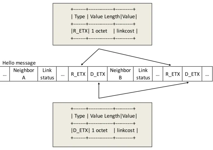
R_ETX TLV and D_ETX TLV formatting is specified in Table 1, whereby the value of the directional link cost is encoded as TimeTLV [27] encoded values with C = 1/1024.

Hello message … Neighbor

A

Link

status … R_ETX D_ETX

Neighbor B

Link

status … R_ETX D_ETX …

Table 3.1 TLV block for R_ETX and D_ETX

The value of the linkcost field of an R_ETX of D_ETX TLV in a HELLO message is set to the R_ETX or D_ETX value of the corresponding link listed in this HELLO message. When a node generated a Hello message, it gets the R_ETX and D_ETX from the link set.

When a node receives a Hello message from its neighbor, it gets the R_ETX and D_ETX value just like getting the link status from the message. Then change the D_ETX value in the link set (now it is the R_ETX in the message) which is corresponding to the generator and the local node and update the 2-neighbor set if needed.

Here, instead of adding 1 TLV carrying ETX value, adding 2 TLVs fits the nature of both link set and 2-neighbor set. For link set, it just needs R_ETX value, because the D_ETX value is computed by the local node. But for the 2-neighbor set, it needs bidirectional ETX values to compute ETX.

+---+---+---+ | Type | Value Length|Value| +---+---+---+ |D_ETX| 1 octet | linkcost | +---+---+---+ +---+---+---+ | Type | Value Length|Value| +---+---+---+ |R_ETX| 1 octet | linkcost | +---+---+---+

21

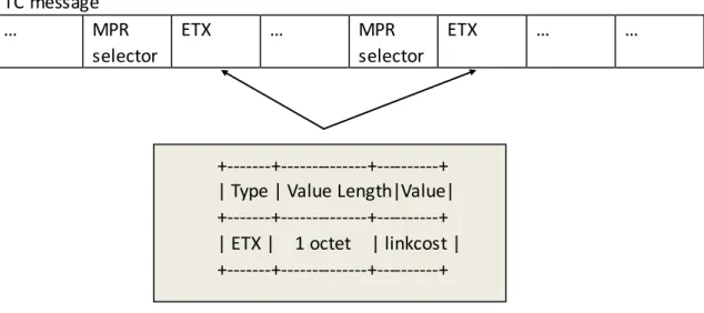
3.2.2 In TC message

TC message helps all the nodes in the network get the ETX value between the message original generator and its MPR selectors. Compared to OLSRv2, one more TLV is added for each address of the MPR selector. The behavior of this kind of message keeps the same.

ETX TLV formatting is specified in table 2 whereby the value of the directional link cost is encoded as TimeTLV [27] encoded values with C = 1/1024.

TC message … MPR selector ETX … MPR selector ETX … …

Table 3.2 TLV block for ETX

The value of the linkcost field of an ETX TLV in a HELLO message is set to the ETX value of the corresponding link listed in this TC message.

Different from Hello message, TC message only carries ETX value (gets from the link set), because the receiver of this message only needs ETX value to update the topology set. It will save the computation of the ETX and reduce the cost of topology control message to add only one TLV (only ETX) instead of 2 (both R_ETX and D_ETX).

3.2.3 Pack and unpack

Before putting ETX value (or D_ETX and R_ETX), we first have to pack it into an 8 bits field using the method in RFC5497. It can encode a quite large range of data, though the accuracy is not very high. Of these 8 bits, the least significant 3 bits represent the mantissa (a), and the most significant 5 bits represent the exponent (b), so that:

value = (1 +

8

) × 2

b

_{× C}

(3.4) +---+---+---+ | Type | Value Length|Value| +---+---+---+ | ETX | 1 octet | linkcost | +---+---+---+

22

code = 8 × b + a

To encode an ETX value t, it works like this:

The minimum that can be represented in this manner is C. In my protocol, C = 1/1024.

The maximum value that can be represented in this manner is 15 × 228 × C, or about 4.0 × 109 × C.

For the receiver, it has to unpack the value first. The way to uncode a 8-bit value m is just the reverse. It is like this:

3.3 Dijkstra algorithm

The multiple-path algorithm is similar to Yi et al. [16] modified Dijkstra algorithm posed in the following:

1. b = m >> 3; 2. a = m - b * 8;

3. ETX = (1 + a/8) * 2^b * C.

1. find the largest integer b such that t/C >= 2^b;

2. set a = 8 * (t / (C * 2^b) - 1), rounded up to the nearest integer;

3. if a == 8, then

set b = b + 1 and set a = 0;

else if 0 <= a <= 7, and 0 <= b <= 31, then

the required time-value can be represented by the time-code 8 * b + a

else

it cannot be represented.

23

But for the ETX link metric, the initial weight of each link (C here) is set to be the corresponding ETX value from link set, 2-neighbor set and the topology set.

MultiPathDijkstra(s, d, G, N) C1 = C G1 = G For i = 1 to N do SourceTreei = Dijkstra(Gi, s) Pi = GetPath(SourceTreei, d) For all arcs e in E

If e is in Pi or Reverse(e) is in Pi then

Ci+1(e) = fp(Ci(e))

Else if the vertex Head(e) is in Pi then

Ci+1(e) = fe(Ci(e))

End if End for

Gi+1 = (V, E, Ci+1)

End for

24

4. Experiment

4.1 QualNet

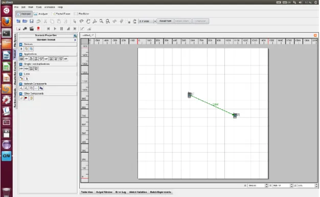
We do all the simulation on QualNet [28], one of the most popular communication simulation platforms for network. Developing a routing protocol is very expensive and complex if the procedures are done in the real world. But now users can do the planning, testing and training on QualNet, which can mimic the behavior of a real communications networks. This is a really economic method for developing, deploying and managing network-centric systems throughout their entire lifecycle. Users can also evaluate the basic behavior of a network. A comprehensive environment for designing protocols, creating and animating network scenarios, and analyzing their performance are included in QualNet.

QualNet is a special simulator for its scenario-based feature. A scenario allows the user to set all the network components and conditions under which the network will operate. They includes terrain details, channel propagation effects such as fading, shadowing and noise, and wired and wireless subnets, network devices including switch, router and etc, and all the protocols and standards in different layers and the applications such as mobile phone running on the network. Most of the setting is optional. Users can easily set the scenario as they wish for further study or just keep the basic setting. Some of the options are already installed when QualNet is first installed, but the users can also configure their own options using C++ or C.

Why QualNet is so popular? The answer is it enables users to design new protocol models, optimize new and existing models, design large wired and wireless networks using pre-configured or user-designed model as well as analyze the performance of networks and perform what-if analysis to optimize them.

QualNet is easy to use thanks to its user-friendly interface. It mainly contains 4 components.

Architect – a graphical scenario design and visualization tool. In Design mode, users

can build their own scenario by setting all the network components and conditions and put all the devices, applications and data streams. This can be done easily by using intuitive, click and drag operations. While in the visualization mode, users can run their own scenario to see how the applications in the network move and how the packets in different layers flow through the network when the scenario is running. The running speed can be modified to fit different demands. Real-time statistics are also an option, where you can view dynamic graphs while a network scenario simulation is running. Every time the simulation is finished, a stat file tracing the

25

packets will be created and saved.

Figure 4.1 Interface of QualNet

Analyzer – a statistical graphing tool that analyzes and displays hundreds of metrics

in different layers collected during the simulation of a scenario (get from the stat file). Users can choose to see pre-designed reports or customize graphs with their own statistics. Multi-experiment reports are also available. All statistics are exportable to spreadsheets in CSV format for further study.

26

Figure 4.2 Analyzer

Packet Tracer -- A graphical tool that provides a visual representation of packet trace

files generated during the simulation of a network scenario. Trace files are text files in XML format that contain information about packets as they move up and down the protocol stack

File Editor -- A text editing tool for all the files needed to make a scenario. Users can

also create or change their scenario using this tool instead of Architect. It is a much easier and faster way if duplicated operations are needed in scenarios making.

What makes QualNet enable creating a virtual network environment are speed, scalability, model fidelity, portability and extensibility.

Speed – QualNet can support real-time speed in 3 modeling: software-in-the-loop, network emulation, and human-in-the-loop modeling. Thanks to faster speed, model developers and network designers can run multiple “what-if” analyses by varying model, network, and traffic parameters in a short time.

Scalability -- QualNet can model thousands of nodes with the help of the latest hardware and parallel computing techniques. To run on cluster, multi-core, and multi-processor systems to model large networks with high fidelity cannot be a challenge for QualNet.

Model Fidelity -- QualNet uses highly detailed standards-based implementation of protocol models. It also includes advanced models for the wireless environment to enable more accurate modeling of real-world networks.

Portability -- QualNet and its library of models run on a vast array of platforms, including Windows and Linux operating systems, distributed and cluster parallel architectures, and both 32- and 64-bit computing platforms. Users can now develop a protocol model or design a network in QualNet on their desktop or laptop Windows computer and then transfer it to a powerful multi-processor Linux server to run capacity, performance, and scalability analyses .

Extensibility – being able to connect to other hardware and software applications, such as OTB, real networks, and third party visualization software makes QualNet greatly enhance the value of the network model.

4.2 Simulations: OLSR vs. MP-OLSR

In this subsection, extended study of comparisons of OLSR and MP-OLSR in different scenarios is done. Expect mobility, background traffic and node density are 2 criteria that we focus on here.

27

4.2.1 Background traffic

p a r a m e t e r v a l u e s p a r a m e t e r v a l u e s simulator Qualnet 5.0 MAC propagation delay uS

routing protocol OLSR and MP-OLSR short packet transmit limit 7 simulation area 1500*1500 m long packet transmit limit 4 mobility RWP, max speed 4 m/s Rtx threshold 0

simulation time 100s physical layer model PHY 802.11b applications CBR wireless channel frequency 2.4GHz application packet size 512 bytes propagation limit -111.0 dBm transmission interval 0.1s pathloss model two ray ground Transport protocol UDP shadowing model constant network protocol IPv4 shodowing mean 4.0dB IP fragmentation unit 2048 transmission range 270m priority input queue size 50000 temperature 290K MAC protocol IEEE 802.11 noise factor 10 receive sensitivity -83 transmission power 15.0 dBm Data rate 11 Mbps

Table 4.1 Simulation parameter set

parameter values

TC interval 5s

HELLO interval 2s

refresh timeout interval 2s

neighbor hold time 6s

topology hold time 15s

duplicate hold time 30s

link layer notification yes number of path in MP-OLSR 3

MP-OLSR fe fe(c) = 2c

MP-OLSR fp fp(c) = 3c

Table 4.2 OLSR and MP-OLSR parameters

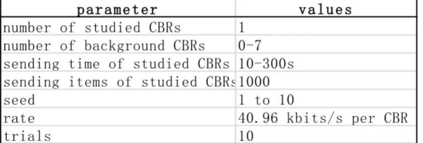
parameter values

number of studied CBRs 1

number of background CBRs 0-7 sending time of studied CBRs 10-300s sending items of studied CBRs1000

seed 1 to 10

rate 40.96 kbits/s per CBR

trials 10

Table 4.3 CBR parameters

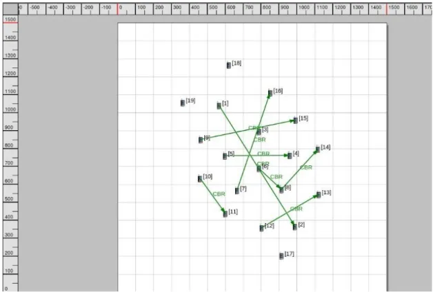
In our 8 scenarios, there are 19 nodes and several CBRs. CBR sent from node 1 to node 2 is the data we want to send. All the other CBRs are regarded as the background. We keep the initial location of each node but increase the background CBR one by one from 0 to 7 to do the simulations to analyze how they influence the QoS of these 2 routing protocols. Figure 4.3 is the scenario with 7 background CBRs.

28

Figure 4.3 Simulation scenario for background traffic with 7 background CBRs

We can see from figure 4.4 that MP-OLSR outperforms OLSR in delivery ratio in dealing the effect of background traffic. The former one keeps the ratio above 85% no matter how heavy the background traffic is, while the latter one keeps it around 70%. Multiple-path, route recovery and loop detection all help to improve it. When the background CBRS increases, the delivery ratio of MP-OLSR decreases. This may be resulted from the longer queue time and the crush of some paths. In terms of standard deviation of delivery ratio, MP-OLSR shows a much more stable performance. For MP-OLSR, the average standard deviation is 0.1, while for OLSR, the value is 0.15. This can be explained by the reduction of instability done by multiple paths.

Figure 4.4 delivery ratio and the corresponding standard deviation in OLSR and MP-OLSR

MP-OLSR also does much better than OLSR in end-to-end delay. Its many be due to the multiple path reducing the queuing time in the intermediate nodes. Route recovery and loop detection also make a difference. With the increasing of

29

background CBRs, the delays of both routing protocols get larger. Compared to MP-OLSR, OLSR has a greater change, especially in 4-background-CBR point. This sharp increment is mainly due to the unique of the scenario. But there is no doubt that MP-OLSR can better deal with an unsatisfying network topology. The standard deviation also supports it: MP-OLSR has a smaller value for standard deviation, especially when there are more than 5 background CBRs.

Figure 4.5 end-to-end delay and the corresponding standard deviation in OLSR and MP-OLSR

We also want to study the cost of topology management needed by these 2 protocols. We compute the cost like this,

Topology management = total bytes of topology messages received

total bytes of topology messages and data received (4.1)

In theory, these 2 routing protocols send out the same number of TC control messages because their topology managing behavior is proactive. But in practice, since MP-OLSR has the route recovery and loop detection, it may send out more TC messages. When there are some changes in the topology, one node may send out a TC message before the end of the constant interval. But since MP-OLSR has a much higher throughput, the percentage of topology messages taken among all the received messages and data may be lower.

Figure 4.6 shows the simulation result of the topology management. From it, we can see that MP-OLSLR actually costs less than OLSR in topology management, but only around 0.4% less. This is resulted from the greater increment in throughput when using MP-OLSR. No matter how heavy the background traffic is, the cost in the studied node keeps quite steady.

30

Figure 4.6 Topology management in OLSR and MP-OLSR

4.2.2 Node density

In this simulation, the simulation parameter and OLSR and MP-OLSR parameters are the same as those in 4.2.1.

parameter value

node density 20,25,30,35,40,45,50,55,60,65,70 nodes/1500m*1500m number of CBRs 3

sending time of CBRs 10-300s sending items of CBRs 1000

seed 1, 3, 4, 10 maximum node mobility 2, 9, 16 m/s simulation time 200s

trials 12

Table 4.4 node density parameters

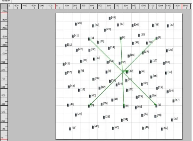
In this part, we use 3 CBRs and keep them unchanged but change the number of nodes by 5 every time from 20 to 70 to study the influence of node density on these 2 routing protocols. All the CBRs are studied. Figure is the scenario of 70 nodes.

31

Figure 4.7 scenario for node density (70 nodes)

From figure 4.8, we observe that when the node density increases, the delivery ratio increases at the beginning and then keeps still. This is because when there are just a few nodes, there may be not enough available paths to send data (both for OLSR and MP-OLSR). With the increment of the nodes, the chance to find an available path or even choose some best paths becomes bigger. But when the node number is big enough, the delivery ratio reach its peak. After that, more nodes and more paths to choose won’t increase the delivery ratio. On the contrast, more topology information will cost the channel source making the delivery ratio a little bit lower. But no matter what the node density is, MP-OLSR keeps a much better performance than OLSR due to its multiple path mechanism. In terms of standard deviation, the former one also keeps a lower degree, because when it uses several paths, the influence of the difference in various scenarios will be lessened, especially at the very beginning, when there are not enough nodes to ensure a good quality of the transmission.

32

Figure 4.8 delivery ratio and the corresponding standard deviation in OLSR and MP-OLSR

When considering the end-to-end delay, MP-OLSR also outperforms OLSR in both the average and the standard deviation, because the multipath mechanism decreases the risk of taking a bad path, which may happen when using OLSRL. It also lessens the impact of various scenarios. This is shown by its lower standard deviation (for MP-OLSR, it is 0.02 and for OLSR it is 0.1). Thus, MP-OLSR has a more stable performance when compared with OLSR.

Figure 4.9 end-to-end delay and the corresponding standard deviation in OLSR and MP-OLSR

No matter how many nodes are there in the network, OLSR costs more than MP-OLSR in topology management. The difference enlarges with the increment of the nodes. This is resulted from the much higher throughput in MP-OLSR. When there are more than 50 nodes, the topology management of OLSR is over 5%, which means it is now a cost protocol. So when the node density is large, it is better to use MP-OLSR.

33

Figure 4.10 topology management in OLSR and MP-OLSR

4.2.3 Conclusion

From the experiment above, we can see that MP-OLSR outperforms OLSR under different criteria like background traffic and node density in terms of delivery ratio, delay and topology management. MP-OLSR also shows its ability in dealing special scenarios.

4.3 Simulations: ETX vs. hop count in MP-OLSR

4.3.1 Background traffic

The parameter sets for this simulation are the same as those in 4.2.1. And the statistics for hop count are the same as those for MP-OLSR in 4.2.1.

From figure 4.11, we can see that the delivery ratio of ETX first increases then decreases. This may be caused by the route recoveries and loop discoveries and the traffic jam. At the very beginning, when there is only one CBR in the network, in some scenarios, we observe an extra number of TC message generated in ETX. So some intermediate nodes may do the route recoveries and loop discoveries after that studied CBR arrived. The delay may make the nodes discard the data packets. It is more serious in ETX, for it has to spend more time waiting for ETX value. Otherwise, it may choose the one or 2 paths only. So ETX performs worse than hop count at the very beginning. When more CBRs join in, the route discovery and loop recovery may already have been done when the background CBRs arrive, so the delivery ratio of the studied CBR increases. But when the background traffic becomes heavier and heavier, there will be traffic jam which resulted in the increment of delay and decrement of delivery ratio for both metric. But generally speaking, ETX does better than hop count to lessen the background traffic effect in our scenarios. This may

34

result from its initiation to find “best” paths. But the difference is not significant. In terms of standard deviation of delivery ratio, ETX shows a more stable performance than hop count, especially in 4, 6 and 7-background-CBR point, for it tries to keep find “best” quality paths in various seeds with various maximum nodes speeds.

Figure 4.11 delivery ratio of ETX and hop count

Where there is more traffic, the intermediate nodes need more time to handle the longer queues. So the end-to-end delay of sending the studied CBR is larger and larger. ETX and hop count perform very similarly expect in scenarios with 4 background CBRs. When considering the standard deviation, we can see a sharp peak for hop count in 4-background-CBR point. We think it just a special case. In other words, these 2 metrics have very similar performances when dealing with background traffic in end-to-end delay. However, ETX can keep the QoS even if there is a special case.

Figure 4.12 end-to-end delay of ETX and hop count

As we mentioned before, MP-OLSR needs more topology management than OLSR due to the route recovery and loop detection. But if it uses ETX as the metric, even more topology managements are required. In the Hello message, for each R_etx or D_etx, one more tlv block is required, while in the TC message, one more tlv block is needed for each ETX value. So in total, there will be much more cost in the topology management for ETX. The followed figure shows the different cost by both metric.

35

Here, ETX costs as 5/3 times as many as hop count does no matter how many background traffic there are. But more CBRs won’t ask for more topology management cost. This is the characteristic of proactive routing protocol.

Figure 4.13 topology management of ETX and hop count

4.3.2 Node density

The parameter sets in this experiment is the same as those in 4.2.2. And the statistics for hop count are the same as those for MP-OLSR in 4.2.2.

From figure 4.14, we can see that when there are more nodes, there is a higher delivery ratio, no matter it uses ETX or hop count. This is because more nodes means more links available to send data. Generally speaking, hop count has a higher delivery ratio than ETX and a little more stable performance no matter how many nodes there are. Because the link qualities of the paths hop count chooses in different seeds are various, while the paths ETX choose in different seeds keep similar quality. This makes hop count shows a higher standard deviation in delivery ratio.

Figure 4.14 delivery ratio of ETX and hop count

These 2 metrics also performs similarly in end-to-end delay. It is very interesting that when the nodes number reach 35, the delay sharply drops down. This may be because when there are 35 nodes, links available are enough for multiple paths for the 3 CBRs, while there are 30 nodes, some chosen paths are duplicated. From the

36

standard deviation, ETX and hop count are once again neck and neck. When there are a few nodes in a wide network (this time the standard deviation is about 0.15), the difference in seeds and speeds make a big different in the performance of MP-OLSR, no matter what metric it uses. But when the nodes are enough, this effect will be lessened (this time the standard deviation is around 0.005). This causes the sharply drop down of standard deviation in 35-node point.

Figure 4.15 end-to-end delay of ETX and hop count

This time ETX still costs more in topology management than hop count. With the increment of node density, the cost increases too. This is because when there are more nodes, there are more Hello message and TC message to send.

Figure 4.16 topology management of ETX and hop count

4.3.3 Mobility

Since we fail to see the advantage to use ETX in the previous experiment, we carry out one more experiment – changing the nodes’ mobility to see whether ETX is better. ETX is designed to consider the link quality and when the mobility is very big, the link quality changes a lot. So ETX is expected to have a better performance in this experiment. Following is the mobility parameter set. Other parameters are the same as the previous experiments.

37 parameter values max speed 5, 10, 15, 20, 25, 30 m/s seed 1--10 number of node 81 number of CBRs 4 CBRs start and end time 15--95s interm sent by CBRs 800/CBR

seed 1 to 10

simulation time 100s

trials 10

Table 4.5 mobility parameter set.

We use the 81-node scenario with 4 CBRs and different maximum speed of nodes (from 5 to 30). Though 30m/s is too fast for ordinary case, for general estimation, we still concern a larger range of mobility change. Figure 4.17 is the scenario of this part.

Figure 4.17 scenario of 81 nodes for mobility study.

In the comparison of delivery ratio, ETX and hop count show the same trend with the increasing of maximum node mobility. The faster the speed is, the lower the delivery ratio is. This is understandable. When the nodes move faster and faster, the probability of breaking links becomes bigger and bigger.

But hop count always keeps a little bit higher delivery ratio then ETX. At 5m/s, they have a similar delivery ratio, but the difference enlarges until the speed reaches 20m/s. Then, it keeps stable. There may be 2 reasons for this. First is the topology of

38

this scenario. At the beginning, our topology of nodes and applications are quite symmetric. Because ETX is a bidirectional symmetrical link metric, some intermediate nodes may choose the same paths. And this will result in a longer queue in the intermediate nodes thus lead to the increment of the delay and then decrement of the delivery ratio. The other reason may be that ETX prefers an “old” best path. Nodes need time to fill the ETX value. If a node just gets part of it (D_etx or R_etx), this link may not be used. So some “actually” best paths won’t be chosen by ETX, but randomly chosen by hop count. The effect of the first reason will be lessened when the mobility increases, for the symmetric topology will be sooner asymmetric. And the effect of the second reason will first enlarge when a faster speed brings more new neighbors to a node and then lessen when a much faster speed makes hop count fail to choose “good” paths randomly while ETX still can choose pretty “good” paths.

In terms of standard deviation, 20m/s is also a special point. Before that, hop count performs more stable than ETX in different seeds, but after that, it becomes more instable. This may be because in low speed, different seeds make the put-off of the ETX serious to different extends. The ETX thus shows a larger deviation. When in high speed, the link qualities of the paths hop count chooses in different seeds are various, while the paths ETX choose in different seeds keep similar quality. This makes hop count shows a higher deviation in delivery ratio. An increasing speed makes the network topology in different seeds more various, thus makes the deviations for both metrics increase too.

Figure 4.18 delivery ratio of ETX and hop count

In case of end-to-end delay, hop count shows better in low speed while ETX does better in high speed. The reasons are similar as those for delivery ratio. In terms of deviation, ETX shows a more stable performance in different seeds.