Pépite | Turbulence intégrable dans des expériences de fibres optiques : dynamique locale et statistique

Texte intégral

(1)Thèse de Alexey Tikan, Université de Lille, 2018. U NIVERSITÉ DE L ILLE D OCTORAL T HESIS. Integrable turbulence in optical fiber experiments: from local dynamics to statistics. Author: Alexey T IKAN. Supervisors: Prof. Pierre S URET Prof. Stéphane R ANDOUX. A thesis submitted in fulfillment of the requirements for the degree of Doctor in the domain of Physics Diluted media and fundamental optics. Thesis defended in front of jury: Prof. Prof. Prof. Prof. Prof. Prof.. G UY M ILLOT S ERGEI T URITSYN S ERGE B IELAWSKI M ARC D OUAY G ENNADY E L S TEFANO T RILLO. University of Burgundy Aston University University of Lille University of Lille Northumbria University University of Ferrara. (referee) (referee) (examiner) (examiner) (examiner) (examiner). November 15, 2018 © 2018 Tous droits réservés.. lilliad.univ-lille.fr.

(2) Thèse de Alexey Tikan, Université de Lille, 2018. © 2018 Tous droits réservés.. lilliad.univ-lille.fr.

(3) Thèse de Alexey Tikan, Université de Lille, 2018. iii. Declaration of Authorship I, Alexey T IKAN, declare that this thesis titled, “Integrable turbulence in optical fiber experiments: from local dynamics to statistics” and the work presented in it are my own. I confirm that: • This work was done wholly or mainly while in candidature for a research degree at this University. • Where any part of this thesis has previously been submitted for a degree or any other qualification at this University or any other institution, this has been clearly stated. • Where I have consulted the published work of others, this is always clearly attributed. • Where I have quoted from the work of others, the source is always given. With the exception of such quotations, this thesis is entirely my own work. • I have acknowledged all main sources of help. • Where the thesis is based on work done by myself jointly with others, I have made clear exactly what was done by others and what I have contributed myself.. Signed: Date:. © 2018 Tous droits réservés.. lilliad.univ-lille.fr.


(5) Thèse de Alexey Tikan, Université de Lille, 2018. v. “Life at low intensity is dull.” Rick Trebino. © 2018 Tous droits réservés.. lilliad.univ-lille.fr.


(7) Thèse de Alexey Tikan, Université de Lille, 2018. vii. UNIVERSITÉ DE LILLE. Abstract Physics Diluted media and fundamental optics Integrable turbulence in optical fiber experiments: from local dynamics to statistics by Alexey T IKAN This work is dedicated to the investigation of the origin of statistical phenomena recently observed in the framework of integrable turbulence. Namely, experimental and numerical studies of the partially- coherent waves propagation in 1-D Nonlinear Schrödinger equation systems revealed a deviation from the Gaussian statistics. Focusing and defocusing regimes of propagation demonstrated qualitatively different behaviour: the probability of extreme events to appear in the focusing case is higher than it is predicted by normal law, while in defocusing it is lower. We provided optical experiments well described by the 1-D Nonlinear Schrödinger equation in order to investigate this problem. We built two novel and complementary ultrafast measurement tools. Employing these tools we provided direct observation of coherent structures which appear at different stages of the propagation in both regimes. Providing analysis of these structures, we determined dominating mechanisms in both focusing and defocusing regimes. In the focusing regime, we discovered the universal appearance of Peregrine soliton-like structures and made a link with the rigorous mathematical result obtained in the semiclassical regime. In the defocusing case, we showed that the mechanism of nonlinear interference of neighbour pulse-like structures defines the evolution of the partially-coherent initial conditions. We considered a simplified model which explained the presence of different scales in the recorded data. Keywords: Nonlinear optics; Ultrafast phenomena - Measurement; Solitons; Optical fibers; Integrable turbulence; Nonlinear statistical optics; Nonlinear Schrödinger equation; Temporal imaging. © 2018 Tous droits réservés.. lilliad.univ-lille.fr.

(8) Thèse de Alexey Tikan, Université de Lille, 2018. viii UNIVERSITÉ DE LILLE. Résumé Physique Milieux dilués et optique fondamentale Turbulence intégrable dans des expériences de fibres optiques: dynamique locale et statistique par Alexey T IKAN Ce travail est dédié à l’étude de l’origine des phénomènes statistiques récemment observés dans le cadre de la turbulence intégrable. Les études expérimentales et numériques de la propagation d’ondes partiellement cohérentes dans les systèmes décrits par l’équation de Schrödinger non linéaire à une dimension ont révélé un écart par rapport à la distribution gaussienne. Les régimes de propagation focalisant et défocalisant présentent un comportement qualitativement différent: la probabilité que des événements extrêmes apparaissent dans le cas focalisant est supérieure à la loi normale, alors que dans le régime défocalisant, elle y est inférieure. Nous avons réalisé des expériences d’optique bien décrites par l’équation de Schrödinger non linéaire 1-D afin d’étudier ce problème. Nous avons construit deux outils de mesure nouveaux et complémentaires. En utilisant ces outils, nous avons réalisé une observation directe des structures cohérentes qui apparaissent à différents stades de la propagation dans les deux régimes. En fournissant une analyse de ces structures, nous avons déterminé les mécanismes dominants dans les régimes focalisant et défocalisant. Dans le régime focalisant, nous avons mis en évidence le caractère universel de structures voisines des solitons de Peregrine et établi un lien avec un résultat mathématique rigoureux obtenu dans le régime semiclassique. Dans le régime défocalisant, nous avons montré que le mécanisme d’interférence non linéaire entre impulsions voisines définit l’évolution des conditions initiales partiellement cohérentes. Nous avons proposé un modèle simplifié qui explique la présence des différentes échelles dans les données enregistrées. Mots clés: Optique non linéaire; Phénomènes ultra-rapides - Mesure; Solitons; Fibres optiques; Turbulence intégrable; Optique statistique non linéaire; Équation de Schrödinger non linéaire; Imagerie temporelle. © 2018 Tous droits réservés.. lilliad.univ-lille.fr.

(9) Thèse de Alexey Tikan, Université de Lille, 2018. ix. Acknowledgements First of all, I would like to thank all the members of the committee for their participation and contribution to the public defence of the current work. Namely, Prof. Guy Millot from the University of Burgundy and Prof. Sergei Turitsyn from Aston University for taking the role of referees; Prof. Serge Bielawski and Prof. Marc Douay from the University of Lille, Prof. Gennady El from Northumbria University and Prof. Stefano Trillo from the University of Ferrara for being my examiners. It is hard to imagine a better committee for this particular work. This would not be possible without all the institutions and organisations involved. Namely, University of Lille directed by Jean-Christophe Camart; Laboratory PhLAM and its director Marc Douay; the Doctoral School SMRE with its coordinator Christophe Van Brussel and director Joël Cuguen, doctoral studies director Cristian Focsa and Majid Taki (former director); Labex CEMPI and particularly Marc Lefranc. Thereby, I would like to thank them. I am afraid that it is barely possible to express all my gratitude to my supervisors Prof. Pierre Suret and Prof. Stephane Randoux. As we agreed, my PhD went in a rather non-usual way. Starting from the first day of my work in Lille, I always had amazingly interesting projects, non-stop. Looking back, I realize that every single moment was an important part of the plan and even working on individual projects I have never been alone. Despite all the variety of research directions you are working on, all the teaching and administrative work, you always always had time to discuss ideas, results or problems. You always shared your passion and will for discovery. I believe that an important basis for the future carer of a scientist is a scientific school. These three years in Lille were my school. It is very pity to leave you. Also, I would like to thank all the group members who helped me. Among them Pierre Walczak who was my first example of the successful thesis defence. His thesis was an important reference that I often read. Another PhD from our team who I would like to thank is Rebecca El Koussaifi. We spent two nice years with Rebecca working side by side. Her ability to work hard is astonishing and at the same time very inspiring. I would like to thank the new generation PhD students: Giacomo Roberti, Adrien Kraych and Alexandre Label. Discussions with them helped me to look differently on the topics that I thought are completely understood. Special thank to Giacomo for explaining me the Boffetta-Osborne algorithm. It was a pleasure to have François Gustave as a postdoc in our team. I would like to thank him for the great job he did in creating a good atmosphere around as well as his help in the automation of our optical sampling oscilloscope. I wish the best to François Copie, a new lecturer, and the new division our team represented by Alberto Amo, Omar Jamadi and Bastian Real Elgueda.. © 2018 Tous droits réservés.. lilliad.univ-lille.fr.

(10) Thèse de Alexey Tikan, Université de Lille, 2018. x Big thanks to all our collaborators! First of all, I would like to thank another team of PhLAM: Prof. Serge Bielawski, Prof. Christophe Szwaj and Clèment Evain. I learned a lot of things from you working on the Time Microscope. Also, I cannot forget the big help of Nunzia Savoia, Marc Le Parquier and Gauthier Dekyndt during this experiment. For almost everything I know about integrable systems, dispersive hydrodynamics and inverse scattering transform I would like to thank Prof. Gennady El. Special thanks for decoding of the Tovbis-Bertola result that was a basis of Chapter 3. I would like to thank Prof. Miguel Onorato for his clear and useful lectures. Also, I would like to thank Dmitry Agafontsev and Andrey Gelash for very helpful and interesting discussions. Support of my friends is what always helped me to keep afloat. Particularly, I would like to thank Tobias Lipfert and Sabine Kopec for being my closest friends all these years and sharing with me all the successes and failures. I will never forget the Sunday Physics Club and Junheng Shi in particular. I hope our ways will cross again. I cannot forget about my Russian friends: Asya; Dima; Vital’ka, Oleg and Sashka; Misha, Igor and Evgen. There are a lot of people who were around and made this time in Lille better: Alexandra, Ambroise, Anna, Dana, Eva, Katharina, Lamyae and others. It is hard to imagine my way in physics without my school teacher Arjamatova Nadejda Antonovna. The fire she has set many years ago is still shining. I hope you will bring to the World many new generations of people who love physics. In the end, I would like to thank my little family for their unconditional and permanent support at my every step.. © 2018 Tous droits réservés.. lilliad.univ-lille.fr.

(11) Thèse de Alexey Tikan, Université de Lille, 2018. xi. Contents Declaration of Authorship. iii. Abstract. vii. Acknowledgements 1. © 2018 Tous droits réservés.. ix. Introduction 1 1.1 Integrable Turbulence . . . . . . . . . . . . . . . . . . . . . . . . 1 1.1.1 Solitary waves and solitons . . . . . . . . . . . . . . . . 1 1.1.1.1 Short history of solitons . . . . . . . . . . . . . 2 1.1.1.2 Equations that have solitonic solutions . . . . 3 1.1.2 Integrable turbulence is not turbulence . . . . . . . . . 4 1.1.2.1 Wave turbulence . . . . . . . . . . . . . . . . . 4 1.1.2.2 Integrable turbulence . . . . . . . . . . . . . . 5 1.1.3 Partially-coherent light . . . . . . . . . . . . . . . . . . . 6 1.1.3.1 Different initial states often considered in the framework of integrable turbulence . . . . . . 6 1.1.3.2 Central limit theorem . . . . . . . . . . . . . . 8 1.1.3.3 Statistical properties of partially-coherent waves 9 1.1.4 Rogue Waves . . . . . . . . . . . . . . . . . . . . . . . . 10 1.1.4.1 Rogue Waves in ocean . . . . . . . . . . . . . 10 1.1.4.2 Rogue Waves in optics . . . . . . . . . . . . . 12 1.2 Nonlinear Schrödinger equation . . . . . . . . . . . . . . . . . 13 1.2.1 Universality of NLS equation . . . . . . . . . . . . . . . 13 1.2.1.1 NLS in optics and other physical systems . . 13 1.2.2 Basic properties of the focusing 1-D NLS . . . . . . . . 15 1.2.2.1 Stationary solutions . . . . . . . . . . . . . . . 15 1.2.2.2 Modulation instability . . . . . . . . . . . . . 17 1.2.2.3 Solitons on the finite background and Rogue Waves . . . . . . . . . . . . . . . . . . . . . . . 19 1.2.3 Basic properties of the defocusing 1-D NLS . . . . . . . 20 1.2.3.1 Dark solitons . . . . . . . . . . . . . . . . . . . 21 1.2.3.2 Dispersive shock waves . . . . . . . . . . . . . 21 1.2.4 Inverse scattering transform . . . . . . . . . . . . . . . . 22 1.2.4.1 Historical background of inverse scattering transform . . . . . . . . . . . . . . . . . . . . . . . . 23 1.2.4.2 Inverse scattering transform of 1-D NLS: ZakharovShabat problem . . . . . . . . . . . . . . . . . 24 1.2.4.3 Finite-gap theory . . . . . . . . . . . . . . . . . 25 1.2.4.4 Examples of the IST spectra . . . . . . . . . . 27. lilliad.univ-lille.fr.

(12) Thèse de Alexey Tikan, Université de Lille, 2018. xii 1.3. 2. © 2018 Tous droits réservés.. Problematic of the study . . . . . . 1.3.1 State of the art: Theory . . . 1.3.2 State of the art: Experiment 1.3.3 Motivation and objectives .. . . . .. . . . .. . . . .. . . . .. . . . .. . . . .. . . . .. . . . .. . . . .. . . . .. . . . .. . . . .. . . . .. . . . .. . . . .. . . . .. 30 30 31 32. Ultrafast measurements of non-periodic optical waves using the Time Microscopy technique 35 2.1 Ultrafast measurements in optics . . . . . . . . . . . . . . . . . 35 2.2 Basics of the Time Microscopy . . . . . . . . . . . . . . . . . . . 41 2.2.1 Principles of temporal imaging . . . . . . . . . . . . . . 41 2.2.1.1 Diffraction - dispersion analogy . . . . . . . . 42 2.2.1.2 Thin lens - time lens analogy . . . . . . . . . . 44 2.2.1.3 Spatial and temporal imaging with a lens . . 45 2.2.1.4 Time Lens . . . . . . . . . . . . . . . . . . . . . 47 2.2.1.5 Spatial and temporal imaging with a microscope . . . . . . . . . . . . . . . . . . . . . . . 48 2.2.2 Experimental realization of the Time Microscope . . . . 49 2.2.2.1 Pump laser . . . . . . . . . . . . . . . . . . . . 49 2.2.2.2 Home-made femtosecond fiber laser . . . . . 51 2.2.2.3 Beam geometry . . . . . . . . . . . . . . . . . 51 2.2.2.4 Treacy compressor . . . . . . . . . . . . . . . . 53 2.2.2.5 Sum frequency generation . . . . . . . . . . . 54 2.2.2.6 Single-shot spectrometer . . . . . . . . . . . . 55 2.2.2.7 Camera specifications, settings and triggering 56 2.2.3 Power profile reconstruction and typical window of measurements . . . . . . . . . . . . . . . . . . . . . . . . . . 56 2.2.3.1 The window of measurements . . . . . . . . . 58 2.2.4 Optimal resolution and compressor tuning . . . . . . . 58 2.2.5 Time calibration . . . . . . . . . . . . . . . . . . . . . . . 60 2.2.5.1 Numerical estimates of time-to-frequency conversion . . . . . . . . . . . . . . . . . . . . . . 62 2.2.6 Aberrations analysis . . . . . . . . . . . . . . . . . . . . 63 2.2.6.1 Influence of aberrations on the resolution estimates . . . . . . . . . . . . . . . . . . . . . . 67 2.3 Heterodyne Time Microscope . . . . . . . . . . . . . . . . . . . 69 2.3.1 Extension of the Time Microscope for the heterodyne phase measurement . . . . . . . . . . . . . . . . . . . . 70 2.3.1.1 Spatial encoding arrangement . . . . . . . . . 71 2.3.1.2 Setup . . . . . . . . . . . . . . . . . . . . . . . 72 2.3.1.3 Beam geometry . . . . . . . . . . . . . . . . . 72 2.3.1.4 CW source . . . . . . . . . . . . . . . . . . . . 74 2.3.2 Heterodyne Time Microscope tuning . . . . . . . . . . 75 2.3.2.1 What is the same in tuning . . . . . . . . . . . 75 2.3.2.2 Tuning at the 0th order of diffraction grating . 76 2.3.2.3 Phase calibration. Importance of the right frequency choice . . . . . . . . . . . . . . . . . . 76. lilliad.univ-lille.fr.

(13) Thèse de Alexey Tikan, Université de Lille, 2018. xiii 2.3.3. 2.4. 3. © 2018 Tous droits réservés.. 2-D snapshot processing for phase and power reconstruction . . . . . . . . . . . . . . . . . . . . . . . . . . . 2.3.3.1 Intensity reconstruction . . . . . . . . . . . . . 2.3.3.2 Phase reconstruction . . . . . . . . . . . . . . 2.3.4 Verification of the retrieval algorithm by reproducing the mean optical spectrum . . . . . . . . . . . . . . . . . Removing aberrations. Spatial Encoding Arrangement with Hologram Observation for Recording in Single-shot the Electric field (SEAHORSE). . . . . . . . . . . . . . . . . . . . . . . . 2.4.1 Setup . . . . . . . . . . . . . . . . . . . . . . . . . . . . . 2.4.2 Phase sign and direction of time axis . . . . . . . . . . . 2.4.3 Comparison between HTM and SEAHORSE . . . . . .. 78 79 80 81. 82 83 84 85. Peregrine soliton as a prototype of rogue waves in the integrable turbulence 89 3.1 Gradient catastrophe in the focusing NLS and its regularisation. Tovbis-Bertola theorem. . . . . . . . . . . . . . . . . . . . 89 3.1.1 Semi-classical limit of the focusing NLS . . . . . . . . . 90 3.1.2 Experimental evidence of the local Peregrine soliton emergence from deterministic initial conditions . . . . . . . 96 3.2 Role of Tovbis-Bertola scenario in dynamics of the partiallycoherent waves . . . . . . . . . . . . . . . . . . . . . . . . . . . 103 3.2.1 Nonlinear propagation of the partially-coherent waves in optical fibre: ultrafast measurements with the HTM and SEAHORSE . . . . . . . . . . . . . . . . . . . . . . 103 3.2.1.1 Numerical simulation of 1-D NLS with partiallycoherent waves . . . . . . . . . . . . . . . . . . 104 3.2.1.2 Adaptation of the HTM and SEAHORSE to the partially-coherent light measurements . . 104 3.2.1.3 Partially-coherent light measurements with the HTM . . . . . . . . . . . . . . . . . . . . . . . . 106 3.2.1.4 Comparison with the numerical simulations . 109 3.2.1.5 Partially-coherent light measurements with the SEAHORSE . . . . . . . . . . . . . . . . . . . . 111 3.2.1.6 Nonlinear Digital Holography . . . . . . . . . 112 3.2.1.7 Comparison of statistical parameters . . . . . 116 3.2.2 Connection between local dynamics and statistics in focusing NLS . . . . . . . . . . . . . . . . . . . . . . . . . 116 3.2.2.1 Numerical estimation of e distribution . . . . 119 3.2.2.2 Calculation of the fourth moment of the PDF 119 3.2.2.3 Results of comparison . . . . . . . . . . . . . . 120 3.3 IST analysis of the experimentally measured PS emerged from the integrable turbulence . . . . . . . . . . . . . . . . . . . . . 121 3.3.1 Fourier collocation method . . . . . . . . . . . . . . . . 123 3.3.2 Global and local approaches to the IST . . . . . . . . . . 124 3.3.2.1 Global IST with zero boundary conditions . . 125 3.3.2.2 Interpretation of the Finite-gap spectrum . . . 125. lilliad.univ-lille.fr.

(14) Thèse de Alexey Tikan, Université de Lille, 2018. xiv. 3.3.3 3.3.4. 3.3.2.3 Role of the window size . . . . . . 3.3.2.4 Role periodization in the local IST IST Analysis of Tovbis-Bertola scenario . . IST of the experimental data . . . . . . . .. . . . .. . . . .. . . . .. . . . .. . . . .. . . . .. . . . .. 129 130 131 135. 4. Integrable turbulence in the defocusing NLS model 139 4.1 Numerical study of the 1-D defocusing NLS integrable turbulence . . . . . . . . . . . . . . . . . . . . . . . . . . . . . . . . . 139 4.1.1 Simulations of the partially-coherent light propagation in 1-D defocusing NLS system . . . . . . . . . . . . . . 140 4.1.2 DSW and dark solitons as fundamental bricks of the 1-D defocusing NLS integrable turbulence . . . . . . . 144 4.1.2.1 Black, grey and high order solitons . . . . . . 144 4.1.2.2 IST approach to the characterisation of the dark solitons . . . . . . . . . . . . . . . . . . . . . . 146 4.1.2.3 Dispersive Shock Wave formation via two pulse collision . . . . . . . . . . . . . . . . . . . . . . 146 4.1.2.4 Generation of the dark solitons . . . . . . . . 150 4.1.3 Statistical approach to the 1-D defocusing NLS integrable turbulence . . . . . . . . . . . . . . . . . . . . . . 151 4.2 Experimental investigation the defoctusing NLS integrable turbulence by using Heterodyne Time Microscope . . . . . . . . . 153 4.2.1 Zoology in the defocusing regime of NLS integrable turbulence . . . . . . . . . . . . . . . . . . . . . . . . . . 154 4.2.2 Experimental data analysis . . . . . . . . . . . . . . . . 156. 5. Conclusions and perspectives. A Thermal Lensing in the Treacy compressor. 161 165. B Estimates of non-linear and dispersion coefficients of the PM fiber 167 C Change of variables in NLS equation. 171. D Intrapulse stimulated Raman scattering effect on the random wave propagation 173 E Evolution of the spectra of the partially-coherent wave in defocusing system. 177 Bibliography. © 2018 Tous droits réservés.. 185. lilliad.univ-lille.fr.

(15) Thèse de Alexey Tikan, Université de Lille, 2018. xv. List of Figures 1.1. 1.2. 1.3. 1.4. 1.5. 1.6. 1.7 1.8. © 2018 Tous droits réservés.. Example of partially-coherent initial condition with finite spectral width and periodic boundary conditions. (a) Representation in the Fourier space. Phase of each Fourier component is an uniformly distributed random variable varying from -π to π. Spectrum was chosen to be Gaussian. (b) Resulting representation in the real space. Creating the signal in the Fourier space we guaranteed periodicity in the real space. Phase experiences the π-jump in the points where power goes to zero. . . Numerically computed distributions of different physical variables following from the Gaussian distribution of the real and imaginary parts of the function describing a random process. (a) Distributions of the real and imaginary part. (b) Uniform distribution of the phase. (c) Rayleigh distribution of the amplitude. (d) Exponential distribution of the intensity. . . . . . . Two branches of stationary solutions of the focusing NLS equation. (top) The dn branch with values of s 0 (blue dotted line), 0.95 (black line), 1 (red dashed line). (bottom) The cn branch. Values of parameter s are the same. . . . . . . . . . . . . . . . . Numerical simulation of the evolution of a plane wave with small noisy perturbation. All units are dimensionless. Brighter colours correspond to higher power. (left) Spatio-temporal diagram showing the modulation instability acting on the quasimonochromatic wave. (right-top) Power profiles at three different cuts of the diagram. Colours are preserved. (rightbottom) Corresponding spectra. . . . . . . . . . . . . . . . . . . Solitons on the finite background plotted using the exact analytical expression. (top-left) Akhmediev breather. (top-right) Kuznetsov-Ma soliton. (bottom) Peregrine soliton . . . . . . . Two dark solitons of different deepness. Black line corresponds to the quasi-black soliton with the value of B close to 1, red dashed line to the gray soliton with B=0.8. (top) Amplitude modulus square. (bottom) Phase profile. . . . . . . . . . . . . . Dispersive shock waves in the double-side dam break problem of 1-D defocusing NLS equation. . . . . . . . . . . . . . . . . . Example of the trace of the monodromy matrix as a function of the eigenvalue ξ. Gray rectangles depict the stable bands. .. 8. 11. 16. 18. 20. 22 23 27. lilliad.univ-lille.fr.

(16) Thèse de Alexey Tikan, Université de Lille, 2018. xvi 1.9. Trace of the monodromy matrix of the dn branch of cnoidal solution of the 1-D focusing NLS equation shown in Fig. 1.3 (top). All colours are preserved. Blue and gray areas show the stable band for the dn(x,0) and dn(x,0.95) respectively. The band of the solitonic solution dn(x,1) converges to the two discrete points -0.5i and 0.5i. . . . . . . . . . . . . . . . . . . . . . 1.10 IST spectra for the dn branch of cnoidal solution of the 1-D focusing NLS equation shown in Fig. 1.3 (top). All colours are preserved. The bands which correspond to dn(x,0) are depicted by blue,for dn(x,0.95) by black and two discrete points of dn(x,1) are depicted by red. . . . . . . . . . . . . . . . . . . . 1.11 Schematic IST spectra of the solitons on the finite background of 1-D focusing NLS equation shown in Fig. 1.5. Arrangement of the figures is preserved. (top-left) Akhmediev breather. (topright) Kuznetsov-Ma soliton. (bottom) Peregrine soliton. . . . 2.1. 2.2. 2.3 2.4 2.5 2.6 2.7 2.8. 2.9. © 2018 Tous droits réservés.. Schemes of the fast optical signal characterization methods. (Top) autocorrelation. A signal divided into two parts. One of them experiences a controllable temporal delay. Two parts are superimposed directly on the photodiode (field autocorrelation) or in a nonlinear crystal (intensity autocorrelation). (Middle) FROG. Similar to the intensity autocorrelation, but instead of the photodiode detection, the spectrum measurements are provided. The resulting FROG trace is a 2-D image of spectrum as a function of delay. (Bottom) SPIDER. A chirped replica of a signal is superimposed with its two copies. The spectrum of the resulting pattern allows to extract the phase and intensity. . . . . . . . . . . . . . . . . . . . . . . . . . . . . Scheme of possible space-time duality realisations. Analogies between paraxial diffraction depicted as cross-section of a free space propagated beam and second-order dispersion in time represented as light beam propagated through a grating compressor or equally in optical fiber in linear regime. Effect of quadratic phase induced by conventional thin lens juxtaposed with nonlinear interaction of a chirped pulse with the studied signal. Also, a possibility of electro-optical phase modulation could be considered as an alternative approach. . . . . . . . . Image formation with space and time lenses. D1 and D2 are dispersions of different values and signs. . . . . . . . . . . . . Image formation with a thin lens. The case of magnification. . Image formation with a microscope. . . . . . . . . . . . . . . . Scheme of the Time Microscope. . . . . . . . . . . . . . . . . . Spectrum of the pump laser after amplification. . . . . . . . . . Schematic illustration of the short pulse amplifier. Picture is taken from the user manual of the Spectra Physics Spitfire amplifier. . . . . . . . . . . . . . . . . . . . . . . . . . . . . . . . . . Scheme of the home-made fiber femtosecond laser. . . . . . . .. 28. 29. 29. 37. 42 46 46 49 50 50. 51 52. lilliad.univ-lille.fr.

(17) Thèse de Alexey Tikan, Université de Lille, 2018. xvii 2.10 Photography of the Treacy compressor. Input beam is depicted by red, output by blue. Beam (red) enters the compressor and reaches necessary hight by the first periscope. After passing through the grating pair (G1 and G2) beam changes its hight on the roof mirror. Reflected beam (blue) path back the grating pair and leaves the compressor by another periscope. Dispersion is controlled by adjusting the distance between the compressor with the high precision motorized translation stage. . 2.11 Scheme of two different monochromatic beams passing through the double-path grating compressor. The beams have close wavelengths λ1 and λ2 . Here θi is initial angle 40◦ , θr (λ) angle between reflected beam and normal to the grating surface. 2.12 Power profile reconstruction of the ASE signal. (a) A typical snapshot obtained with a Time Microscope. (b) Line with a maximum overall power (the 5th line in the picture a). (c) Average TM response envelope of a corresponding set (green) and the maximum overall power line with subtracted background. 2.13 Window of measurements. (a) Result of division of the signal by the envelope the Fig. 2.12c. (b) Retrieved signal shrieked to the window of measurement. The window is chosen symmetrically from the maximum of the envelope. . . . . . . . . . . . 2.14 Resolution curve. Dependence of pulse durations measured with the TM as a functions of distance between grating in the 1560 nm Treacy compressor. Input pulses are produced homemade femtosecond laser presented in the section 2.2.2.2. Each value has been determined by fitting with a Gaussian-like function. The minimum value corresponds to 250 f s for FWHM. . 2.15 Experimental measurements of ≈ 70 f s pulse with the TM. (a) Raw image recorded with the TM. (b) Pulse profile obtained making a cross-section of the image above. . . . . . . . . . . . 2.16 (a)Time microscope response to a series of two pulses (700 f s long) with known spacing. This gives the correspondence between pixel spacing and time: 71 f s/pixel. Note that the lower scale has been defined after this calibration has been made. (b) Corresponding spectrum. The spectral width between 5 peaks is 0.89 THz, which gives the spacing 5.6 ps . . . . . . . . . . . 2.17 Simulation of the Time Microscope. (a) blue pulses of 70 f s are taken as initial signal. Orange pulse of 30 f s is the pump. (b) the same signals experienced dispersion: 0.23 ps2 for the pump and the same but negative for the signal. Usage of these parameters simulates experiments described in the articles [190, 200] . . . . . . . . . . . . . . . . . . . . . . . . . . . . . . . . . .. © 2018 Tous droits réservés.. 53. 55. 57. 59. 60. 61. 62. 65. lilliad.univ-lille.fr.

(18) Thèse de Alexey Tikan, Université de Lille, 2018. xviii 2.18 Simulation of the Time Microscope. Effect of the 3rd order dispersion on the signal detection. (a,e) the ideal case, no higher order dispersion therm is added. (b,f) 3rd order dispersion is added to the initial signal depicted by blue in the Fig. 2.17. (c,g) Show the effect when higher order dispersion term is added to the pump onlt. (d,h) depicts the case when 3rd order dispersion is added to the signal and pump together. The value of the 3rd order dispersion is always the same 5.14 × 10−4 ps3 . This value is computed with the formula 2.20. . . . . . . . 2.19 (a)Root mean square of the pulses measured with the Time Microscope [200], versus distance between grating planes in the 1560 nm compressor. Input pulses are produced by a 70 f s Erbium doped fiber-laser. The minimum value corresponds to ∼250 f s at the full with at the half maximum. Blue dots show every RMS value taken into the account, (b-d) show the superposition of several pulses measured at the given grating distance (b-3.4 cm, c-3.85 cm, d-5.2 cm). . . . . . . . . . . . . . . 2.20 Simulation of the compressor tuning. (a-i) show the signal measured with a simulated Time Microscope with the different distance between gratings of the signal compressor, while the pump compressors stay untouched. Green dashed lines represent the ideal case when only the 2nd order dispersion is added, black lines show the same, but with the presence of the 3rd order dispersion. 3rd order dispersion of the pump is fixed, while the dispersion coefficients of the signal were recomputed according to the formulas 2.16 and 2.20. . . . . . . . 2.21 Experimentally measured dependence of the fifty highest amplitude pulses root mean square on its position on the recorded frame. Distance between the grating was varied from 3.37 cm to 5.15 cm. Optimal distance is 3.85 cm. Data correspond to one depicted in the Fig. 2.19a. The frame center is at 256th pixel. 2.22 Typical snapshot obtained with a spatial encoding arrangement setup. Picture is generated numerically. . . . . . . . . . . 2.23 Experimental setup of Heterodyne Time Microscope arrangement for amplitude and phase measurement of arbitrary signals. (a) Complete setup. (b) Detailed 3-D view of the setup. . 2.24 Recorded spectra of the amplified continuous wave reference. The central wavelength is chosen at the maximum of amplified spontaneous emission noise. . . . . . . . . . . . . . . . . . . . . 2.25 Snapshots recorded at the zero order of the diffraction grating with the time microscope. (a) Line corresponding to the signal alone, (b) reference alone, (c) signal and reference together. The optimal tuning corresponds to symmetric line of the width close to 1 pixel. . . . . . . . . . . . . . . . . . . . . . . . . . . .. © 2018 Tous droits réservés.. 66. 67. 69. 70 71. 73. 75. 76. lilliad.univ-lille.fr.

(19) Thèse de Alexey Tikan, Université de Lille, 2018. xix 2.26 Monochromatic wave phase measurements. Raw images (top) and retrieved phase evolutions (middle) obtained when the signal comes from a monochromatic laser source with various wavelengths, from left to right: λS = 1555.37 nm, λS = 1559.37 nm, λS = 1561.37 nm, λS = 1563.37 nm and λS = 1567.37 nm .In all cases the wavelength of the reference is fixed to λ R = 1561.37 nm. Bottom layer shows the recovered intensity profile. The noise related to the interference of the spontaneous emission of amplifier and monochromatic signal. Corresponding spectra are depicted in the Fig. 2.24. . . . . . . . . . . . . . 2.27 Intensity reconstruction. (a) 2-D snapshot obtained with the HTM. (b) Power profile before division by the envelope (red) and envelope (green). (c) Reconstructed power profile after division by envelope. . . . . . . . . . . . . . . . . . . . . . . . . 2.28 Phase reconstruction. (a) A 2D snapshot of a non-periodic signal. (b) Intensity profile along the green vertical line depicted above. (c) Corresponding Fourier spectra of the intensity profile. By the red dot highlighted the Fourier mode, argument of which is extracted. . . . . . . . . . . . . . . . . . . . . . . . . . 2.29 Phase, amplitude and spectrum of partially coherent waves (ASE). a–f, The width ∆ν of the (average) optical spectrum of the partially coherent light waves emitted by an ASE source is adjusted by using a programmable filter. Results correspond to ∆ν = 0.1 THz (a,c,e,g) and ∆ν= 0.7 THz (b,d,f,h). a,b, Typical raw images recorded by the sCMOS camera of the HTM for ASE light with a spectral width ∆ν = 0.1 THz (a) and ∆ν = 0.7 THz (b). c,d, Phase retrieved from the interference pattern. e,f, Optical power normalized to the average power. In contrast to the raw signal in a and b, the signal in e and f is divided by the average power(P(t)/ < P >). g,h, Optical spectra corresponding to ∆ν = 0.1 THz and ∆ν = 0.7 THz, respectively. Red stars represent the spectrum computed from the averaged Fourier transform of the envelope of the electric field recorded with the HTM. The spectrum recorded by the OSA is plotted with black lines for comparison. . . . . . . . . . . . . . . . . . . 2.30 Spatial Encoding Arrangement with Hologram Observation for Recording in Single shot the Electric field (SEAHORSE). (a) scheme of experimental setup adapted for the double pulse measurements. (b,c,d) Corresponding 2-D snapshot with the temporal hologram, retried phase and power. (e) The image reconstruction by adjusting the second order dispersion coefficient. (f) Reconstructed sharp image of the double-pulse signal. 2.31 Comparison between HTM and SEAHORSE. Single 70 f s pulse obtained with HTM (red) and SEAHORSE after reconstruction (black). . . . . . . . . . . . . . . . . . . . . . . . . . . . . . . . .. © 2018 Tous droits réservés.. 77. 78. 80. 82. 84. 86. lilliad.univ-lille.fr.

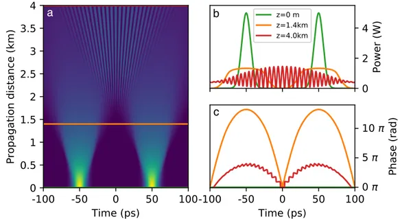
(20) Thèse de Alexey Tikan, Université de Lille, 2018. xx 2.32 Interpolation of the SEAHORSE hologram. A 70 f s pulse recorded with the SEAHORSE. (Black line) pulse reconstructed directly from the hologram, the same as one depicted in Fig. 2.31. (Blue dots) 1024 points zero padding in the Fourier space. (Green dots) the same but with 8192 points. . . . . . . . . . . . . . . . 87 3.1 3.2. 3.3. 3.4. 3.5 3.6 3.7 3.8. 3.9. © 2018 Tous droits réservés.. Second derivative of the sech2 function. . . . . . . . . . . . . . 92 Dynamics of the bell-like shaped initial condition in the NLS system under the dispersionless limit. ρ and u profiles are displayed for ξ = 0, 0.35 and 0.5. Original figure can be found in [216]. . . . . . . . . . . . . . . . . . . . . . . . . . . . . . . . . 92 Analytical formula of the Peregrine soliton. (a) Spatio-temporal diagram. (b-c) Cross-section of amplitude and phase profile at the maximum compression point (ξ = 0). . . . . . . . . . . . . 94 Numerical simulation of the focusing NLS equation. Behaviour at the gradient catastrophe point. Parameter e in the simulation is equal to 1/20. (a,b,c) Spatio-temporal diagram, amplitude and phase cross-section at the maximum compression point. 20sech(τ ) function is taken as initial condition. (d,e,f) the same but for the solitonless potential. 20sech(τ ) exp[−iµ log(cosh(τ ))], here µ = 2. . . . . . . . . . . . . . . . . . . . . . . . . . . . . . . 95 Principal scheme of the experiment implying optical sampling oscilloscope. . . . . . . . . . . . . . . . . . . . . . . . . . . . . . 97 Detailed scheme of optical sampling oscilloscope (top). Signal sampling via sum frequency generation (bottom). . . . . . . . 98 Spectral filtering and propagated pulse spectrum. . . . . . . . 99 Results of experimental measurement of a pulse profile at the point of the gradient catastrophe with the optical sampling oscilloscope. Blue circles and green stars show the measured data before propagation in the fiber and at the gradient catastrophe point, the black line is analytical Peregrine soliton formula applied without a fit, red line corresponds to numerical simulations of the experimental data taken as initial conditions while assuming a constant phase. . . . . . . . . . . . . . . . . . 101 Measurements of a single pulse power and phase profiles in an optical fiber with the frequency-resolved optical gating technique. (top) FROG traces measured at different propagation distances using the cut-back technique. (middle and bottom) corresponding power and phase profiles. Measurements are provided in Institut FEMTO-ST, CNRS Université BourgogneFranche-Comté, Besançon, France. . . . . . . . . . . . . . . . . 102. lilliad.univ-lille.fr.

(21) Thèse de Alexey Tikan, Université de Lille, 2018. xxi 3.10 Simulations of the random wave propagation in the focusing NLS system. Simulation parameters are close to the experimental: β 2 = -20 ps2 /km and γ = 2.4 W −1 km−1 , average power P0 = 2.6 W and spectral width ∆ν = 0.1 THz. (a) Spatiotemporal diagram. Green and orange lines correspond to 0 and 160 m respectively. Orange line shows the distance at which the first localised structure is appearing (-23 ps). (b) Power profile around the maximum of the first localised structure and initial conditions at the same time. Colours are conserved. An application of the Peregrine soliton formula is depicted with red lines. (c) The same (as b) for the phase profile. 105 3.11 Experimentally measured spectra. (a) Original spectrum of ASE light source (blue) and power spectral density of signals after filtering and amplification. (b) the same in the log-scale and zoomed around the 192 THz. . . . . . . . . . . . . . . . . . 107 3.12 Recording of ASE emitted signal with the HTM. (a-d) Demonstrate the typical snapshots of the ASE signal and corresponding phase and power profiles. The spectral widths of the recorded signal were 0.05, 0.1, 0.5, 0.7 THz (depicted from left to right). 107 3.13 Experimentally measured spectra of the partially-coherent signal having the initial width 0.1 THz after propagation in the 400 m PM fiber. (a) Spectra of the output signal with different average powers (0.5, 1, 2.6 and 4 W) (b) same as in a, in log-scale.109 3.14 Observation of the different stages of formation of the localized Peregrine soliton with HTM. Initial partially-coherent light has 0.05 THz spectral width and 0.5 W average power. Snapshots are recorded at the output of the 400 m PM fiber. . . . . . 110 3.15 Nonlinear random waves measured with the HTM setup. (a) Scheme of experiment. Partially-coherent light filtered and amplified is injected into the PM fiber and detected with the HTM. (b-e) Snapshots of the random waves recorded with the HTM, recovered phase (blue) and amplitude (red) profiles. (fi) Corresponding numerical simulations demonstrating the same power and phase profiles. . . . . . . . . . . . . . . . . . . . . . 111 3.16 Partially-coherent light measurement with the SEAHORSE technique. The partially-coherent light after propagation in 400 m PM fiber having the same initial conditions as one depicted in the Fig. 3.15. The first row: ’temporal holograms’ of random waves, recorded using the SEAHORSE. The second and third rows: extracted phase and intensity profiles without postprocessing. The power unit is here the number of electrons detected by sCMOS sensor. The fourth and fifth rows: numerically retrieved phase and intensity profiles by using the digital holography algorithm. . . . . . . . . . . . . . . . . . . . . . . . 113. © 2018 Tous droits réservés.. lilliad.univ-lille.fr.

(22) Thèse de Alexey Tikan, Université de Lille, 2018. xxii 3.17 Nonlinear Digital Holography. Spatio-temporal diagram reconstruction using the experimentally recorded data with the HTM at the output of the 100 m PM fiber (a-f) and at the input (g-l). . . . . . . . . . . . . . . . . . . . . . . . . . . . . . . . . . . 115 3.18 Comparison of the probability density function computed for the partially-coherent light of 0.1 THz spectral width and 2.6 W average power. . . . . . . . . . . . . . . . . . . . . . . . . . . . 117 3.19 Example of the initial conditions processing. 500 ps -long window of 0.05 THz spectral width and 2.6 W power. (Blue line) is the power profile of the partially-coherent wave. (Magenta dots) are detected maxima above the threshold (green dashed line). (Red and green stars) show the left and ring side of the structure at the level of FWHM. . . . . . . . . . . . . . . . . . . 120 3.20 Comparison of the Peregrine-soliton-like structure maximum compression point distribution and the M4 moment at different propagation distances. Partially-coherent initial conditions 0.05 THz and 2.6 W. . . . . . . . . . . . . . . . . . . . . . . . . . 121 3.21 Comparison of the Peregrine-soliton-like structure maximum compression point distribution and the M4 moment at different propagation distances. Partially-coherent initial conditions 0.1 THz and 2.6 W. . . . . . . . . . . . . . . . . . . . . . . . . . 122 3.22 Comparison of the Peregrine-soliton-like structure maximum compression point distribution and the M4 moment at different propagation distances. Partially-coherent initial conditions 0.2 THz and 2.6 W. . . . . . . . . . . . . . . . . . . . . . . . . . 122 3.23 Spatio-temporal diagram of two-soliton u = 2sech( x ) (top) and solitonless u = 2sech( x )exp(−i2µ log(cosh( x ))) with µ = 2 solutions of NLS. (Right) The cross-section of the spatio-temporal diagram for the power and phase. (green) initial conditions, (orange) maximum compression point. Simulations are presented using the normalization of Eq. 3.2. . . . . . . . . . . . . 126 3.24 ZS spectra of the two-soliton (green) and corresponding solitonless (red) potentials. The vertical axis corresponds to the imaginary part of ξ, while horizontal to its real part. . . . . . . 127 3.25 Spatio-temporal diagram of ten-soliton u = 10sech( x ) (top) and solitonless u = 10sech( x )exp(−i10µ log(cosh( x ))) with µ = 2 solutions of NLS. (Right) The cross-section of the spatiotemporal diagram for the power and phase. (green) initial conditions, (orange) maximum compression point. Simulations are presented using the normalization of Eq. 3.2. . . . . . . . . 128 3.26 ZS spectra of the two-soliton (green) and corresponding solitonless (red) potentials. The vertical axis corresponds to the imaginary part of ξ, while horizontal to its real part. . . . . . . 129 3.27 Artificially created IST spectra of the a complex solution of NLS (left) and the Peregrine soliton (right). . . . . . . . . . . . 130. © 2018 Tous droits réservés.. lilliad.univ-lille.fr.

(23) Thèse de Alexey Tikan, Université de Lille, 2018. xxiii 3.28 Effect of the window size on the IST spectra. (left)The Peregrine soliton truncated to the windows [-2,2] blue, [-5,5] green, [-10,10] red. (right) Corresponding IST spectra, the colour is preserved. The chosen window was periodized 30 times. The vertical axis corresponds to the imaginary part of ξ, while horizontal to its real part. . . . . . . . . . . . . . . . . . . . . . . . . 131 3.29 Effect of the periodization on the IST spectra. (left)The Peregrine soliton truncated to the window [-10,10]. (right) IST spectra of the signal. (blue dots) without periodization, (green stars) periodized 5 times and (red crosses) 10 times. The vertical axis corresponds to the imaginary part of ξ, while horizontal to its real part . . . . . . . . . . . . . . . . . . . . . . . . . . 132 3.30 Change of the IST spectrum with the evolution coordinate. (left) Initial amplitude profile ψ(0, τ ) = sech(τ ) with e = 0.02blue, amplitude profiles at different propagation points ξ = 0.42, 0.53, 0.54, 0.543-red and corresponding phase profile -blue. (left) IST analysis with at different positions with fixed window size and periodization number. Similar figure is presented in the book [216]. . . . . . . . . . . . . . . . . . . . . . . . . . . 133 3.31 Conservation of global IST. (left) spatio-temporal diagram for ψ(0, τ ) = sech(τ ) with e = 1/15. (right-top) intensity profile of the initial condition (green) , at the maximum compression point (orange), truncated for the IST computation (red). (rightbottom) global (green, orange) and local (red) IST spectra. The vertical axis corresponds to the imaginary part of ξ, while horizontal to its real part. Colours are preserved. . . . . . . . . . . 134 3.32 Local IST spectra of the local high-amplitude structure which emerges as a regularisation of the gradient catastrophe with different solitonic content (from 3 to 17 solitons). (left) the full IST spectra, (right) zoomed around the unstable band. The vertical axis corresponds to the imaginary part of ξ, while horizontal to its real part. . . . . . . . . . . . . . . . . . . . . . . . . 135 3.33 IST of the experimental data. For the investigation the data from the Fig. 3.17c,d is taken. (left) normalized power profile (black) and the window for IST analysis (red). (right) corresponding IST spectrum. The vertical axis corresponds to the imaginary part of ξ, while horizontal to its real part. . . . . . . 136 3.34 Comparison of the local IST spectra of experimentally measured data and numerically obtained from deterministic initial conditions. (red dots) the same spectrum as in the Fig. 3.33, (blue crosses) from Fig. 3.32 for N =5. The spectra are scaled in order to provide the comparison. . . . . . . . . . . . . . . . 137 3.35 IST of the experimental data. The data is taken from the Fig. 3.15e. (left) normalized power profile (black) and the window for IST analysis (red). (right) corresponding IST spectrum. The vertical axis corresponds to the imaginary part of ξ, while horizontal to its real part . . . . . . . . . . . . . . . . . . . . . . . . . . 137. © 2018 Tous droits réservés.. lilliad.univ-lille.fr.

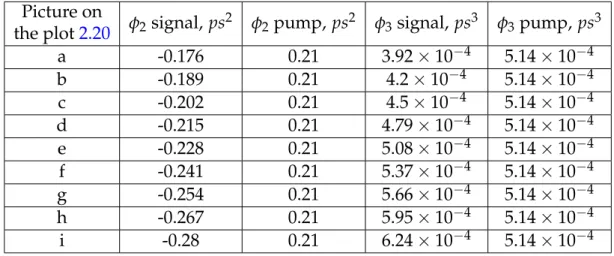
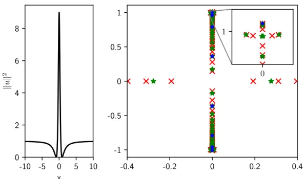
(24) Thèse de Alexey Tikan, Université de Lille, 2018. xxiv 4.1. 4.2. 4.3. 4.4. 4.5 4.6. © 2018 Tous droits réservés.. Simulations of the partially-coherent wave propagation in the defocusing NLS system. Simulation parameters are close to the experimental ones: β 2 = 22 ps2 /km and γ = 3 W −1 km−1 , average power P0 = 4.5 W and spectral width ∆ν = 0.05 THz. (a) Spatio-temporal diagram. Green,orange and red lines correspond to 0, 0.5 and 1 km respectively. Orange line shows the distance at which the double shock happens. (b) Power profile is zoomed around the double shock area. Colours are preserved. (c) The same for the phase profile. . . . . . . . . . . Simulations of the partially-coherent wave propagation in the defocusing NLS system. Simulation parameters are close to the experimental ones: β 2 = 22 ps2 /km and γ = 3 W −1 km−1 , average power P0 = 4.5 W and spectral width ∆ν = 0.1 THz. (a) Spatio-temporal diagram. Green,orange and red lines correspond to 0, 0.52 and 1 km respectively. Orange line shows the distance at which the double shock happens. (b) Power profile is zoomed around the double shock area. Colours are preserved. (c) The same for the phase profile. . . . . . . . . . . Simulations of the partially-coherent wave propagation in the defocusing NLS system. Simulation parameters are close to the experimental ones: β 2 = 22 ps2 /km and γ = 3 W −1 km−1 , average power P0 = 4.5 W and spectral width ∆ν = 0.5 THz. (a) Spatio-temporal diagram. Green and red lines correspond to 0 and 1 km respectively. (b) Power profile is zoomed around the double shock area. Colours are preserved. (c) The same for the phase profile. . . . . . . . . . . . . . . . . . . . . . . . . . . Simulations of the mulisoliton propagation in the defocusing NLS system, u(0, x ) = Ntanh( x ) with N = 4 in this case. Simulations provided for the dimensionless 1-D NLS 4.2. (a) Spatio-temporal diagram. Green, orange and red lines correspond to 0, and 6 nonlinear lengths respectively. (b) Power profile around zoomed around the double shock area. Colours are preserved. (c) The same for the phase profile. . . . . . . . . IST spectra of N soliton solutions . . . . . . . . . . . . . . . . . Simulations of the double pulse signal propagation in the defocusing NLS system. Simulation parameters are close to the experimental ones: β 2 = 22 ps2 /km and γ = 3 W −1 km−1 , peak power P0 = 5 W and separation 30 ps. (a) Spatio-temporal diagram. Green, orange and red lines correspond to 0, 0.44 and 2 km respectively. (b) Power profile is zoomed around the double shock area. Colours are preserved. (c) The same for the phase profile . . . . . . . . . . . . . . . . . . . . . . . . . . . . .. 141. 142. 143. 145 147. 148. lilliad.univ-lille.fr.

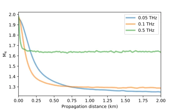
(25) Thèse de Alexey Tikan, Université de Lille, 2018. xxv 4.7. 4.8. 4.9 4.10. 4.11. 4.12. 4.13. 4.14. 4.15. © 2018 Tous droits réservés.. Simulations of the double pulse signal propagation in the defocusing NLS system. Simulation parameters are close to the experimental ones: β 2 = 22 ps2 /km and γ = 3 W −1 km−1 , peak power P0 = 5 W and separation 50 ps. (a) Spatio-temporal diagram. Green, orange and red lines correspond to 0, 0.75 and 2 km respectively. (b) Power profile is zoomed around the double shock area. Colours are preserved. (c) The same for the phase profile. . . . . . . . . . . . . . . . . . . . . . . . . . . . . 149 Simulations of the double pulse signal propagation in the defocusing NLS system. Simulation parameters are close to the experimental ones: β 2 = 22 ps2 /km and γ = 3 W −1 km−1 , peak power P0 = 5 W and separation 100 ps. (a) Spatio-temporal diagram. Green, orange and red lines correspond to 0, 1.4 and 4 km respectively. (b) Power profile is zoomed around the double shock area. Colours are preserved. (c) The same for the phase profile. . . . . . . . . . . . . . . . . . . . . . . . . . . . . 150 Typical scenario of generation of the dark soliton in the defocusing integrable turbulence. . . . . . . . . . . . . . . . . . . . 151 The fourth order moments (M4 [ X ] = E[( X )4 ]/( E[( X )2 ])2 ) of the partially-coherent initial condition as a function of the propagation distance. The average power is 4.5 W, spectral widths 0.05 (blue line), 0.1 (orange) and 0.5 (green) THz. . . . . . . . . 152 Comparison of he fourth order moment (orange) and the FWHM of the spectrum (blue) plotted as a function of the propagation distance. The average power of the partially-coherent initial conditions is 4.5 W, spectral widths - 0.1 THz. Black line shows the position of the maximum of the blue curve (z = 0.23 km). . 153 Experimentally recorded with HTM partially-coherent waves propagated in 900 m fiber with normal dispersion. The initial spectral with is 0.05 THz, average power 4.5 W. (first row) snapshots recorded directly with the HTM. (second and third rows) reconstructed phase and power profiles. . . . . . . . . . 155 Experimentally recorded with HTM partially-coherent waves propagated in 900 m fiber with normal dispersion. Exactly the same experimental parameters as in Fig. 4.12 are used, however in this figure we present data that contains fast oscillating wavetrains. . . . . . . . . . . . . . . . . . . . . . . . . . . . . . . 156 Experimentally recorded with HTM partially-coherent waves propagated in 900 m fiber with normal dispersion. Spectral width is 0.1 THz, average power is 4.5 W. (first row) snapshots recorded directly with the HTM. (second and third rows) reconstructed phase and power profiles. . . . . . . . . . . . . . 157 Experimentally recorded with HTM partially-coherent waves propagated in 900 m fiber with normal dispersion. Spectral width is 0.5 THz, average power is 4.5 W. (first row) snapshots recorded directly with the HTM. (second and third rows) reconstructed phase and power profiles. . . . . . . . . . . . . . 157. lilliad.univ-lille.fr.

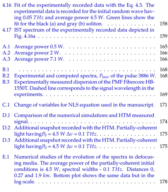
(26) Thèse de Alexey Tikan, Université de Lille, 2018. xxvi 4.16 Fit of the experimentally recorded data with the Eq. 4.3. The experimental data is recorded for the initial random wave having 0.05 THz and average power 4.5 W. Green lines show the fit for the black (a) and gray (b) soliton. . . . . . . . . . . . . . 158 4.17 IST spectrum of the experimentally recorded data depicted in Fig. 4.16a . . . . . . . . . . . . . . . . . . . . . . . . . . . . . . . 159 A.1 Average power 0.5 W. . . . . . . . . . . . . . . . . . . . . . . . 165 A.2 Average power 2 W. . . . . . . . . . . . . . . . . . . . . . . . . 166 A.3 Average power 7.1 W. . . . . . . . . . . . . . . . . . . . . . . . 166 B.1 . . . . . . . . . . . . . . . . . . . . . . . . . . . . . . . . . . . . 168 B.2 Experimental and computed spectra, Pmax of the pulse 3886 W. 168 B.3 Experimentally measured dispersion of the PMF Fibercore HB1550T. Dashed line corresponds to the signal wavelength in the experiments. . . . . . . . . . . . . . . . . . . . . . . . . . . . . . 169 C.1 Change of variables for NLS equation used in the manuscript.. 171. D.1 Comparison of the numerical simulations and HTM measured signal. . . . . . . . . . . . . . . . . . . . . . . . . . . . . . . . . . 174 D.2 Additional snapshot recorded with the HTM. Partially-coherent light havingP0 = 4.5 W ∆ν = 0.1 THz. . . . . . . . . . . . . . . . 175 D.3 Additional snapshot recorded with the HTM. Partially-coherent light havingP0 = 4.5 W ∆ν = 0.1 THz. . . . . . . . . . . . . . . . 175 E.1 Numerical studies of the evolution of the spectra in defocusing media. The average power of the partially-coherent initial conditions is 4.5 W, spectral widths - 0.1 THz. Distances 0, 0.27 and 1.9 km. Bottom plot shows the same data but in the log-scale. . . . . . . . . . . . . . . . . . . . . . . . . . . . . . . . 178. © 2018 Tous droits réservés.. lilliad.univ-lille.fr.

(27) Thèse de Alexey Tikan, Université de Lille, 2018. xxvii. List of Tables 2.1. 2.2 2.3. 2.4. © 2018 Tous droits réservés.. Comparison of the existing ultra-short pulse measurements techniques. In the column Disadvantages we discuss reasons why this technique could not be applied to the partially-coherent waves measurements. For the primary sources of information see [134, 142, 146, 168, 172]. . . . . . . . . . . . . . . . . . . . . Details of numerical simulations for the Fig. 2.18 . . . . . . . . Details of numerical simulations depicted in the Fig. 2.20. Parameters match exactly the configuration of the TM presented in [200]. . . . . . . . . . . . . . . . . . . . . . . . . . . . . . . . . Summary of the estimated vertical and horizontal diameter of the pump, signal and reference beams inside the optical crystal.. 40 65. 68 74. lilliad.univ-lille.fr.


(29) Thèse de Alexey Tikan, Université de Lille, 2018. xxix. List of Abbreviations ASE BBO CW DFT DSW FROG FWHM HTM IST KdV MI NLS OPO OSA OS PBS PDE PDF PMF RMS RW sCMOS SEA SEAHORSE. SFG SG SPIDER TM WSF WS WT ZS. © 2018 Tous droits réservés.. Amplified Spontaneous Emission Beta barium borate Continuous Wave Dispersive Fourier Transform Dispersive Shock Wave Frequency Resolved Optical Gating Full Width at Half Maximum Heterodyne Time Microscope Inverse Scattering Transform Korteweg-deVries Modulation Instability Nonlinear Schrödinger Optical Parametric Oscillator Optical Spectrum Analysers Optical Sampling Polarization Beam Splitter Partial Differential Equation Probability Density Function Polarization Maintaining Fiber Root Mean Square Rogue Wave scientific Complementary Metal-Oxide-Semiconductor Spatial Encoding Arrangement Spatial Encoding Arrangement with Hologram Observation for Recording in Single-shot the Electric field Sum Frequency Generation Sine-Gordon Spectral Phase Interferometry for Direct Electric-field Reconstruction Time Microscope What (it) Stands For Wave Shaper Wave Turbulence Zakharov-Shabat. lilliad.univ-lille.fr.


(31) Thèse de Alexey Tikan, Université de Lille, 2018. 1. Chapter 1. Introduction 1.1. Integrable Turbulence. In this section, we will introduce the framework of our study. The integrable turbulence is a field of the classical physics initiated recently by V.E. Zakharov [1]. The integrable turbulence, rigorously saying, is not turbulence in its classical form [2]. Without loss of generality, it can be understood as studying of complex behaviour of random initial conditions, which can be found behind a dispersive nonlinear partial-differential equation integrable with the inverse scattering method [3, 4] 1 . One of remarkable features of this kind of equations is the localised particlelike solutions called solitons. They play a crucial role in understanding of the corresponding complex dynamics. We will describe some properties of the solitonic solution and show the difference with other solitary waves. Another remarkable feature is the existence of an infinite number of constant of motion. These equations can be integrated by the so called inverse scattering transform. In general, this complex behaviour strongly depends on the initial state of a system. Therefore, at the end of this section, we will explain the particular choice of our random initial conditions and show its basic statistical properties.. 1.1.1. Solitary waves and solitons. Solitons are isolated particle-like travelling waves which are solutions of certain partial differential equations. By its nature, soliton can be determined as a wave that preserves its structure during the propagation due to the interplay between dispersion (or diffraction in 2-D case) and nonlinearity of the system. The property which makes solitons similar to particles is elastic collision. Indeed, like particles, two solitons (asymptotically) restore their initial shapes after the collision, maybe besides some phase shift. Below, we will give a short review of the history of solitons and solitary waves and show some important equations which have solitonic solutions. 1 The. © 2018 Tous droits réservés.. basics of this method will be explained later in Sec. 1.2.4.. lilliad.univ-lille.fr.

(32) Thèse de Alexey Tikan, Université de Lille, 2018. 2. Chapter 1. Introduction. 1.1.1.1. Short history of solitons. Since the time when the first known soliton was observed by J. Scott Russell more than 180 years have passed. Riding a horse along a narrow barge channel, he noticed "a large solitary elevation, a rounded, smooth and welldefined heap of water, which continued its course along the channel apparently without change of form or diminuation of speed" [5]. After providing an experimental investigation of this phenomenon, he made several remarkable conclusions. Except the confirmation of the existence of the solitary water waves, he managed to find a ratio between the speed of the wave, its amplitude and the water depth. However, the theory developed at that moment didn’t allow to predict such object and the works of Russell were a subject to criticism. Rehabilitation of the solitary wave came with works of Dutch scientists Diederik J. Korteweg and his student Gustav de Vries [6], who found in 1895 the equation most accurately describing the main effects observed by Russell. They derived a rather simple equation(known as KdV) for waves in shallow water and found its periodic wave solutions (expressed in terms of Jacobi elliptic functions) which in the asymptotic limit of large wavelengths give a solitary wave. However, further progress in this field came only in 60 years this with the development of the computers. E. Fermi, J. Pasta and S. Ulam studied an anharmonic lattice with quadratic and cubic nonlinearities [7]. They expected a full thermalisation of the system, i.e. uniform redistribution of the energy along different modes. M. Tsingou provided for them a numerical experiment integrating one period of a simple cosine function with periodic boundary conditions. The results of the numerical study surprised researchers. Instead of expected thermalisation, they observed that energy was distributed among only few modes and didn’t show any mixing. Moreover, the system demonstrated a tendency of periodical recurrence to the initial state. This phenomenon is known today as Fermi-Pasta-Ulam-Tsingou recurrence. In order to understand this effect, Kruskal and Zabusky studied a continuous analogue of this model. The corresponding equation was exactly the one derived by Korteweg and de Vries almost 70 years ago for shallow water waves! The periodic solutions and the solitary wave of KdV equation were well known at that time. However, Kruskal and Zabusky pointed out a very remarkable property of solitons, which was not known before. Namely, the fact that two solitons collide elastically, asymptotically recovering its initial shape. By analogy with particles, they coined the term soliton. We will use this property to draw a line between the solitons and other solitary waves. Thereby, we define the soliton as: • Isolated, localized in space travelling wave • Which preserves its shape in time • And collides elastically with other solitons, except maybe a phase shift To other localized travelling waves we will refer as solitary waves. More detailed intoduction to the theory of solitons can be found in the book of M. Ablowitz and H. Segur [3], review of the solitons in [8].. © 2018 Tous droits réservés.. lilliad.univ-lille.fr.

(33) Thèse de Alexey Tikan, Université de Lille, 2018. 1.1. Integrable Turbulence 1.1.1.2. 3. Equations that have solitonic solutions. After the discovery, solitons (as well as solitary waves) were observed in many different systems [3, 9]. Soliton family can be divided in two big classes: conventional and envelope solitons. The solitons observed by Russell in the water channel (KdV equation) are of the first type. The fundamental envelope solitons can be seen as a localised group of waves moving together and preserving its envelope. The definition given above can be applied to the envelope solitons as well. There are a lot of partial-differential equations modelling dispersive nonlinear media which have solutions in the form of the solitary wave. However, not all of them can be called solitons. As we mentioned before existence of solitonic solution is directly related to integrablility of the equations. In [10] reader can fined a (short) list of different kinds of integrable equations with solitonic solutions. This full list is still being replenished. Here we will consider three (relatively) simple and very general equations. KdV equation. As we have seen the first soliton was observed in the media governed by the KdV equation, but it is not the only one historically important event associated with this equation. The method of integrating the nonlinear partial-differential equations known as Inverse Scattering Transform (IST) was shown on the example of KdV as well [11]. We will discuss this method later in Sec. 1.2.4. From the integration of the KdV equation, a new period of nonlinear physics has started. The KdV equation can be written in the form: ut + 6uu x + u xxx = 0. Which describes the evolution of a function u in time t. The second term represents nonlinear part and the third one - dispersion. Fundamental solitonic solution can be written as: u = 2k2 sech2 k ( x − 4k2 t − x0 ), where k and x0 are constants. This solution represents a bell shaped localised wave similar to one observed by Russell. As we now, solitons can be observed in the shallow water, but KdV equation is universal. So the range of its applicability is much wider. As an example we can give ion-acoustic waves in plasma [12], liquid-gas bubble mixture [13], atmospheric Rossby waves [14], etc. Remarkably, the 2-dimensional versions of the KdV called KadomtsevPetviashvili equations are also integrable and, hence, also has family of solitonic solutions [15, 16]. Sine-Gordon (SG) equation. Another historically important equation called Sine-Gordon was derived in the framework of differential geometry. It brought into the soliton theory a widely used Bäcklund transformation. Bäcklund derived it studying surfaces of constant Gaussian curvature in 1880. Knowing solution of one partial differential equation (PDE) we find solutions of another one if there is a corresponding Bäcklund transformation. Its variation called auto-Bäcklund transformation allows to recurrently reconstruct. © 2018 Tous droits réservés.. lilliad.univ-lille.fr.

(34) Thèse de Alexey Tikan, Université de Lille, 2018. 4. Chapter 1. Introduction. the whole hierarchy of solitons. The SG equation can be expressed as follows: utt − u xx + sin(u) = 0 Integrability of the SG equation was first proved by Ablowitz Kaup Newell and Segur [17]. For the list of applications of the SG equation we refer reader to review of Scott, Chu and McLaughlin [8]. Nonlinear Schrödinger (NLS) equation. This equation we will study in details in the present manuscript. We will discuss later in this chapter (see Sec. 1.2). This equation has maybe the widest range of applications among the equations discussed in the section. In the 1-dimensional case it is usually written as follows: iut + u xx + 2σ|u|2 u = 0. where σ = ±1. The case when σ = 1 NLS equation called focusing (see Sec. 1.2.2), σ = −1 respectively defocusing (see Sec. 1.2.3). NLS equation was integrated by V.E. Zakharov and A. B. Shabat [18]. This equation has an exact solution in the form of the envelope soliton. NLS equation found its applications in deep-water wave dynamics [3, 19, 20], electro-magnetic waves in media with third order nonlinearity [21], magnetic spin waves [22], plasma physics [18], etc. Hasegawa and Tappert [23, 24] first derived the NLS equation in fiber optics. In the presented manuscript we will consider complex dynamics of light in optical fibers and demonstrate emergence of some particular envelope solitons. Remarkably, also it’s generalized version called Vector NLS which can be represented as a set of N coupled 1-D NLS equations: ! N. iu jt + u jxx + 2. ∑ σn |un |2. uj = 0. n =1. can be integrated in the case when N = 2 and σ1 = σ2 = 1. This system is known as Manakov model [25]. It can be applied to the fibers with constant birefringence [26].. 1.1.2. Integrable turbulence is not turbulence. From the general point of view, "wave turbulence" names all the complex phenomena arising from the nonlinear propagation of random waves [27]. In this sense, integrable turbulence can be seen as a peculiar case of wave turbulence. However, in the standard form of the wave turbulence theory, the dynamics is dominated by the resonant interaction. On the contrary, as we’ll see below, no resonant interaction exist in the integrable turbulence [28]. 1.1.2.1. Wave turbulence. Wave turbulence (sometimes called weak turbulence) theory studies dynamics of weakly nonlinear and dispersive random waves [27, 29]. It is originated from the pioneering work of R. Peierls [30], where he describes the. © 2018 Tous droits réservés.. lilliad.univ-lille.fr.

(35) Thèse de Alexey Tikan, Université de Lille, 2018. 1.1. Integrable Turbulence. 5. kinetics (including the evolution of spectrum and probability density function of amplitude) of phonons in anharmonic crystals. Later, the approach of wave turbulence found its application in plasma physics [31, 32], hydrodynamics [33, 34], optics [35–37] and many different areas of physics. Below, we cite a definition of the wave turbulence given in the book of S. Nazarenko [27]: "Wave turbulence (WT) can be generally defined as out-ofequilibrium statistical mechanics of random nonlinear waves". Also, further in this book we can find an important refinement: "Notably, the WT language, i.e. triad or quartic resonant wave interactions, is sometimes also used to qualitatively describe situations where waves are not so weak and when formally the WT theory is invalid." Presence of the resonant interactions is the key difference between the standard wave turbulence and integrable turbulence. Usually, in the WT approach, it is common to eliminate the nonresonant terms by providing a canonical transformation. 1.1.2.2. Integrable turbulence. Studying the complex evolution of random initial conditions in the integrable equations one has to take into the account nonresonant interaction terms [36]. Indeed, the linear dispersion relation2 k (ω ) doesn’t have nontrivial resonances. As a consequence, we do not find direct or inverse energy cascades and related effects observed in the WT framework. However, the presence of the solitonic content, instabilities and gradient catastrophes leads to a variety of not trivial effects, which will be widely discussed in the present manuscript. This problem was considered in the work of P.A.E.M. Janssen in the framework of the water waves [38]. He studied a narrowband limit of deterministic Zakharov equation [39] which describes the potential flow if the ideal fluid of infinite depth. This limit leads to the Nonlinear Schrödinger equation. The author describes the evolution of the spectrum as well as the fourth order moment of amplitude probability density functions. He proved an important statement that statistics deviates from Gaussian, which is not possible without taking into the account nonresonant terms. Let’s demonstrate the absence of the resonances in the quasi-linear case of 1-D NLS equation3 . The linear dispersion relation can be expressed as k = − βω 2 . Therefore, we obtain the set of equations describing the conservation of energy and momentum: ( ω12 + ω22 = ω32 + ω42 (1.1) ω1 + ω2 = ω3 + ω4 2 Reader. has to take into the account that notations used in hydrodynamics (therefore in the wave turbulence) are different from ones used in optics. The dispersion relation in hydrodynamics is written as ω (k). The reason is the following change of variables: t → z and x → τ. z and τ variable are convenient for the description of the optical experiments, where z can be considered as fiber length and τ is the time. 3 It is easy to show that for the higher dimension (or generalised one-dimension [40]) version of NLS equation the WT approach can be fully applied [37, 41]. © 2018 Tous droits réservés.. lilliad.univ-lille.fr.

(36) Thèse de Alexey Tikan, Université de Lille, 2018. 6. Chapter 1. Introduction. Inverting this to (. (ω1 + ω3 )(ω1 − ω3 ) = (ω4 + ω2 )(ω4 − ω2 ) ω1 − ω3 = ω4 − ω2. Finally, we see that the system 1.1 has only trivial solutions: ( ( ω1 = ω4 ω1 = ω3 or ω2 = ω3 ω2 = ω4. (1.2). (1.3). However, the resonances could occur in this system due to the nonlinear effects. For example, exponential growth of a perturbation of a monochromatic wave known as modulation instability (see Sec. 1.2.2.2) can be considered as a consequence of nonlinear phase-matching [21].. 1.1.3. Partially-coherent light. The choice of random initial conditions may significantly affect the behaviour of the system governed by dispersive nonlinear PDE. Here, we provide a short overview of widely used random initial conditions. For our studies, we have chosen a particular case of a partially-coherent wave with Gaussian statistics. These initial conditions are of particular importance in different physical systems. Finally, we present general statistical properties of partially-coherent waves, essential for understanding the results of the present work. 1.1.3.1. Different initial states often considered in the framework of integrable turbulence. The randomness of initial conditions naturally appears in majority of real experiments. Particularly in optics, one can encounter an optical noise of different origin: from slow thermal fluctuations to the shot noise, caused by the discrete nature of light. All these effects are stochastic and, hence, have to be studied with statistical methods. Generally, the random process can be considered as a certain superposition of random variables. The theory of the random processes knows many different examples, however, in the framework of the integrable turbulence, the process of paramount importance is the complex Gaussian process [42]. This importance is related to the fact that many physical processes can be considered as a supposition of large number of independent random variables. According to the central limit theorem (which we show in the next section) such superposition leads to the Gaussian statistics [42]. In such processes, real and imaginary parts of the random function have Gaussian distributions. Integrable turbulence studies the evolution of such random initial signal in the nonlinear dispersive media. As an example, we can give random superposition of water waves in the ocean or photons with random phases in the amplified spontaneous emission source propagated in an optical fiber.. © 2018 Tous droits réservés.. lilliad.univ-lille.fr.