Homogenous and heterogeneous logical proportions

O

pen

A

rchive

T

OULOUSE

A

rchive

O

uverte (

OATAO

)

OATAO is an open access repository that collects the work of Toulouse researchers and makes it freely available over the web where possible.

This is an author-deposited version published in : http://oatao.univ-toulouse.fr/ Eprints ID : 13108

To cite this version : Prade, Henri and Richard, Gilles Homogenous and

heterogeneous logical proportions. (2014) The IfCoLog Journal of

Logics and their Applications, Vol. 1 (n° 1). pp. 1-52. ISSN 2055-3706

Any correspondance concerning this service should be sent to the repository administrator: staff-oatao@listes-diff.inp-toulouse.fr

Homogenous and Heterogeneous Logical

Proportions

Henri Prade and Gilles Richard

Université Paul Sabatier IRIT

1

Introduction

Commonsense reasoning often relies on the perception of similarity as well as dis-similarity between objects or situations. Such a perception may be expressed and summarized by means of analogical proportions, i.e., statements of the form “A is to B as C is to D”. Analogy is not a mere question of similarity between two objects (or situations), but rather a matter of proportion or relation between objects. This view dates back to Aristotle and was enforced by Scholastic philosophy. Indeed, an analogical proportion equates a relation between two objects with the relation between two other objects. As such, the analogical proportion “A is to B as C is to

D” poses an analogy of proportionality by (implicitly) stating that the way the two

objects A and B, otherwise similar, differ is the same way as the two objects C and

D, which are similar in some respects, differ.

A propositional logic modeling of analogical proportions, viewed as a quaternary connective between the Boolean values of some feature pertaining to A, B, C, and

D, has been recently proposed in [14]. This logical modeling amounts to precisely

state that the difference between A and B is the same as the one between C and

D, and that the difference between B and A is the same as the one between D and C. This view can then be proved to be equivalent to state that each time a Boolean

feature is true for A and D (resp. A or D) it is also true for B and C (resp. B or

C), and conversely. This latter point shows that a counterpart of a characteristic

behavior of numerical geometrical proportions (a_b = _dc), or of numerical arithmetic proportions (a − b = c − d), namely that the product (resp. sum, in the second case) of the extremes is equal to the product (resp. the sum) of the means, is still observed in the logical setting.

However, analogical proportions are not the only type of quaternary statements relying on the ideas of similarity and dissimilarity that can be imagined. They turn out to be a special case of so-called logical proportions [17]. Roughly speaking, a

logical proportion between four terms A, B, C, D equates similarity or dissimilarity evaluations about the pair (A, B) with similarity or dissimilarity evaluations about the pair (C, D). A set of 120 distinct logical proportions, whose formal expressions share the same structure as well as some remarkable properties, has been identified. Among them, 8 logical proportions stand out as being the only ones that enjoy a code independency property. Namely, their truth status remains unchanged when the truth values 0 and 1 are exchanged. These 8 proportions split into two groups, namely, 4 homogeneous ones (which include the analogical proportion) [22], and 4

heterogeneous logical proportions, which are dual in some sense of the former ones.

The pairs (A, B) and (C, D) play symmetrical roles for homogeneous proportions, while it is not the case for the heterogeneous ones. However, both enjoy noticeable permutation properties.

Similarity and dissimilarity are naturally a matter of degrees. Thus, the exten-sion of homogeneous and heterogeneous logical proportions when features are graded make sense in a multiple-valued logic setting. This makes these logical proportions closer to a symbolic counterpart of numerical proportions where the equality between ratios or differences of quantities may be approximate.

Besides, knowing three values, the statement of the equality of numerical ratios, or of numerical differences, involving a fourth unknown value, and expressing a proportionality relation, is useful for extrapolating this latter value. Similarly, the solving of logical proportion equations may be the basis of reasoning procedures. In particular, when an analogical proportion holds for a large number of features between four situations described by means of n binary features, one may make the plausible inference that the same type of proportion should also hold for a (n + 1)th feature. If the truth value of this latter feature is known for three of the situations, and unknown for the fourth one, this value can thus be obtained as the solution of an analogical proportion equation.

The paper is organized as follows. In Section 2, the notion of logical proportions is introduced and formally defined. Then, a structural typology of the different families of logical proportions, as well as some noticeable properties, are presented. Section 3 is devoted to a more detailed study of homogeneous proportions. Section 4 deals with extensions of homogeneous proportions for handling non Boolean or unknown features. This is the case if the features are gradual, or if they are binary but may not apply. It may also happen that for some situations it is not known if a feature holds or not. The section investigates these three types of cases (gradual features, features non applicable, and missing information about a feature), where different multiple-valued logical calculi are involved. Section 5 focuses on heteroge-neous proportions, studies their properties, and their extension to gradual properties. Section 6 discusses applications of homogeneous and heterogeneous proportions.

Ho-mogeneous logical proportions, especially analogical proportions, seem of interest for completing missing values in tables, a problem sometimes termed “matrix abduc-tion” [1]. It amounts in the logical proportion setting to completing a series A, B,

C with X such as (A, B, C, X) makes a proportion of a given type. Heterogeneous

logical proportions are shown to be instrumental for picking out the item that does not fit in a list. Thus, the setting of logical proportions appears to be rich enough for coping with two different types of reasoning problems where the ideas of similarity and dissimilarity play a key role in both cases. Psychological quizzes or tests are used for illustrating this ability to exploit comparisons in reasoning.

This paper provides a synthesis of results that have appeared mostly in a series of papers by the authors [19, 18, 22].

2

Logical proportions

Before introducing the formal definitions, let us briefly clarify the notations used. • When dealing with Boolean logic, a, b, . . . denote propositional variables

(hav-ing 0 or 1 as truth value), and we use the standard symbols ∧, ∨ to build up formulas (with parentheses when needed). For the negation operator, instead of using the standard ¬ symbol, we will use a to denote ¬a. This is done for saving space when writing long formulas. As usual ⊤ (resp. ⊥) denotes the always true (resp. false) proposition.

• 0 and 1 denote the Boolean truth values, and a valuation v is just a function from the set of propositional variables to the set of truth values, i.e., {0, 1} in the Boolean case, or [0, 1] in the graded case.

• When we propose a new definition, we will use the symbol , meaning defini-tional equality. The right hand side of the equation is the definition of the left hand side.

• When we consider syntactic identity, we use =Id: for instance a ∧ b =Id a ∧ b

but we do not have a ∧ b =Idb ∧ a.

• Finally, the symbol ≡ is reserved for the equivalence, i.e.,

a → b, a ∨ b a ≡ b, (a → b) ∧ (b → a)

Logical proportions are Boolean formulas built upon what we called indicators. We introduce this concept in the next subsection and we investigate some fundamental properties.

2.1 Similarity and dissimilarity indicators

Generally speaking, the comparison of two items A and B relies on the representation of these items. For instance, the items may be represented as a set of features A and B. Then, one may define a similarity measure. This is the aim of the well-known work of Amos Tversky [26], taking into account the common features, the specificities of A w.r.t. B, and the specificities of B w.r.t. A, respectively modeled by A ∩ B, A \ B, and B \ A. Here, we are not looking for any global measure of similarity, we are rather interested in keeping track in what respect items are similar and in what respect they are dissimilar using Boolean indicators. This is why we adopt a logical setting: features are viewed as Boolean properties. Let P be such a property, which can be seen as a predicate: P (A) may be true (in that case ¬P (A) is false), or false.

When comparing two items A and B w.r.t. such a property P , it makes sense to consider A and B similar (w.r.t. property P ):

- when P (A) ∧ P (B) is true or - when ¬P (A) ∧ ¬P (B) is true. In the remaining cases:

- when ¬P (A) ∧ P (B) is true or - when P (A) ∧ ¬P (B) is true,

we can consider A and B as dissimilar w.r.t. property P .

Since P (A) and P (B) are ground formulas, they can simply be considered as Boolean variables, and denoted a and b by abstracting w.r.t. P . If the conjunction

a ∧ b is true, the property is satisfied by both items A and B, while the property is

satisfied by neither A nor B if a ∧ b is true. The property is true for A only (resp. B only) if a ∧ b (resp. a ∧ b) is true. This is why we call such a conjunction of Boolean literals an indicator, and for a given pair of Boolean variables (a, b), we have exactly 4 distinct indicators:

• a ∧ b and a ∧ b that we call similarity indicators, • a ∧ b and a ∧ b that we call dissimilarity indicators.

Let us observe that negating anyone of the two terms of a dissimilarity indicator turns it into a similarity indicator, and conversely. Hence, negating the two terms of an indicator yields an indicator of the same type.

2.2 Building logical proportions with indicators

When describing two elementary situations encoded by two Boolean variables a and

relation with what takes place with two other Boolean variables c and d in terms of some indicator, leads to state an equivalence between one indicator pertaining to the pair (a, b) and one indicator pertaining to the pair (c, d). However, one may consider that using two indicators to describe the status of 2 variables a and b may be more satisfactory from some symmetrization point of view than using only one indicator. For instance, using a ∧ b together with a ∧ b establishes the symmetry between a and

b, or using a ∧ b together with a ∧ b considers counter-examples as well as examples

in context a, or using a ∧ b together with a ∧ b provides the same role to negative or positive features. Note that such symmetrizations occur for free with numerical proportions where for instance one can exchange a and b on the one hand, c and d on the other hand, still writing a unique equality. It is why we more particularly focus on proportions defined as the conjunction of two distinct equivalences between an indicator for the pair (a, b) and an indicator for the pair (c, d).

One may wonder about the simultaneous use of three indicators for comparing two Boolean variables. This would lead to three equivalences instead of two, which appears conceptually more complicated, and maybe farther from the idea of propor-tion inherited from the numerical setting. Then, for the sake of simplicity, we stick to the conjunctions of two equivalences between indicators in the following. This defines a so-called logical proportion [17, 19]. More formally, let us denote I(a,b) and I′

(a,b)1 (resp. I(c,d) and I(c,d)′ ) 2 indicators for (a, b) (resp. (c, d)). Then

Definition 1. A logical proportion T (a, b, c, d) is the conjunction of 2 distinct equiv-alences between indicators of the form

I_(a,b)≡ I_(c,d)∧ I′

(a,b)≡ I(c,d)′

An example of such proportion is ((a ∧ b) ≡ (c ∧ d)) ∧ ((a ∧ b) ≡ (c ∧ d)) where • I(a,b) , a ∧ b, I(c,d) , c ∧ d,

• I′

(a,b) , a ∧ b, I(c,d)′ , c ∧ d.

Obviously, this formal definition goes beyond what may be expected from the infor-mal idea of “logical proportion”, since equivalences may be put between things that are not homogeneous (i.e., mixing similarity and dissimilarity indicators in various ways).

Let us first determine the number of logical proportions. To build an equivalence between indicators, we have to choose one indicator among four for the pair (a, b)

1_{Note that I}

(a,b)(or I(a,b)′ ) refers to one element in the set {a ∧ b, a ∧ b, a ∧ b, a ∧ b}, and should

and similarly for the pair (c, d), we get 4 × 4 = 16 distinct equivalences. To build up a logical proportion, we first choose one equivalence among 16, and then the second equivalence has to be chosen among the 15 remaining ones, leading to 16 × 15 = 240 pairs of equivalences. Taking into account the commutativity of the Boolean conjunction, we finally get 240/2 = 120 potentially distinct logical proportions . We shall see in subsection 2.4 that they are indeed distinct. We first provide a syntactic typology of the logical proportions.

2.3 Typology of logical proportions

Logical proportions can be classified according to the ways they are built up. At this stage, it makes sense to distinguish between two types of indicators: similarity indicators that are denoted by S, and dissimilarity indicators that are denoted by

D: e.g., D_(a,b) ∈ {a ∧ b, a ∧ b}.

Depending on the way the indicators are chosen, one may mix the similarity and the dissimilarity indicators differently in the definition of a proportion.

This leads us to distinguish a specific subfamily of proportions, the so-called

degenerated proportions: those ones involving only 3 distinct indicators in their

definition. For instance

(a ∧ b ≡ c ∧ d) ∧ (a ∧ b ≡ c ∧ d) is such a proportion where I_(c,d) =IdI_(c,d)′ .

For the remaining proportions, it is required that all the indicators appearing in the definition of the proportion are distinct. At this stage, among the non-degenerated proportions, we can identify 4 subfamilies that we describe below:

• The 4 homogeneous proportions

For these proportions, we do not mix different types of indicators in the 2 equivalences. The homogeneous proportions are of the form

S_(a,b) ≡ S_(c,d)∧ S′

(a,b)≡ S(c,d)′

or

D_(a,b) ≡ D_(c,d)∧ D′

(a,b) ≡ D′(c,d)

Thus, it appears that only 4 proportions among 120 are homogeneous. They are (with their name):

– analogy : A(a, b, c, d), defined by

– reverse analogy: R(a, b, c, d), defined by

((a ∧ b) ≡ (c ∧ d)) ∧ ((a ∧ b) ≡ (c ∧ d)) – paralogy : P (a, b, c, d), defined by

((a ∧ b) ≡ (c ∧ d)) ∧ ((a ∧ b) ≡ (c ∧ d)) – inverse paralogy: I(a, b, c, d), defined by

((a ∧ b) ≡ (c ∧ d)) ∧ ((a ∧ b) ≡ (c ∧ d))

Analogy already appeared under this form in [14]; paralogy and reverse analogy were first introduced in [16], and inverse paralogy in [19]. While the analogical proportion (analogy, for short) reads “a is to b as c is to d” and expresses that “a differs from b as c differs from d, and conversely b differs from a as

d differs from c”, reverse analogy expresses that “a differs from b as d differs

from c, and conversely b differs from a as c differs from d”, paralogy expresses that “what a and b have in common, c and d have it also” (positively and negatively). Paralogy is a given name. Finally, inverse paralogy expresses that “what a and b have in common, c and d miss it, and conversely”. As can be seen, inverse paralogy expresses a form of antinomy between pairs (a, b) and (c, d). Note that we use two different words, “inverse” and “reverse”, since the changes between analogy and reverse analogy on the one hand, and paralogy and inverse paralogy on the other hand, are not of the same nature. From now on, we denote analogy with A, reverse analogy with R, paralogy with P , inverse analogy with I. When we need to denote any unspecified proportion, we will use the letter T .

• The 16 conditional proportions

Their expression is made of the conjunction of an equivalence between simi-larity indicators and of an equivalence between dissimisimi-larity indicators. Thus, they are of the form

S_(a,b)≡ S_(c,d)∧ D_(a,b) ≡ D_(c,d)

There are 16 conditional proportions (2 × 2 choices per equivalence). An example is

Let us explain the term “conditional”. It comes from the fact that these pro-portions express “equivalences” between conditional statements. Indeed, it has been advocated in [5] that a rule “if a then b” can be seen as a three valued entity that is called ‘conditional object’ and denoted b|a [4]. This entity is:

– true if a ∧ b is true. The elements making it true are the examples of the rule “if a then b”,

– false if a∧b is true. The elements making it true are the counter-examples of the rule “if a then b”,

– undefined if a is true. The rule “if a then b” is then not applicable. Thus, the above proportion ((a ∧ b) ≡ (c ∧ d)) ∧ ((a ∧ b) ≡ (c ∧ d)) may be denoted b|a :: d|c combining the two conditional objects in the spirit of the usual notation for analogical proportion. Indeed, it expresses a semantical equivalence between the 2 rules “if a then b” and “if c then d” by stating that they have the same examples, i.e. (a ∧ b) ≡ (c ∧ d)) and the same counter-examples (a ∧ b) ≡ (c ∧ d).

It is worth noticing that such proportions have equivalent forms, e.g.: (b|a :: d|c) ≡ (b|a :: d|c)

which agrees with the above semantics and more generally with the idea of conditioning. Indeed the examples “if a then b” are the counter-examples of “if a then b”, and vice-versa. Due to this remark, it is enough to consider the equivalences between one of the 4 conditional objects a|b, b|a, a|b, b|a, and the 4 other conditional objects built with (c, d), yielding 4 × 4 proportions as expected. Besides, 8 conditional proportions have been first considered in [19], but not the 8 remaining ones, since they do not satisfy the “full identity” property, discussed in the next section.

• The 20 hybrid proportions

They are characterized by equivalences between similarity and dissimilarity indicators in their definitions. They are of the form.

S_(a,b)≡ D_(c,d)∧ S′

(a,b) ≡ D′(c,d)

or

D_(a,b) ≡ S_(c,d)∧ D′

or

S_(a,b)≡ D_(c,d)∧ D_(a,b) ≡ S_(c,d).

There are 20 hybrid proportions: 2 of the first type, 2 of the second type, 16 of the third type since we have here 4 choices for an equivalence S_(a,b) ≡ D_(c,d), and 4 choices for D_(a,b) ≡ S_(c,d).

If we remember that negating anyone of the two terms of a dissimilarity indi-cator turns it into a similarity indiindi-cator, and conversely, we understand that changing a into a (and a into a), or applying a similar transformation with respect to b, c, or d, turns

- an hybrid proportion into an homogeneous or a conditional proportion; - an homogeneous or a conditional proportion into an hybrid proportion. This indicates the close relationship of hybrid proportions with homogeneous and conditional proportions. More precisely,

- on the one hand there are 4 hybrid proportions such that replacing a with a leads to the 4 homogeneous proportions A, R, P , I. They are obtained by the two first kinds of patterns for building hybrid proportions. Moreover, we shall see in the next section that they constitute with the 4 homogeneous propor-tions the 8 proporpropor-tions that are the only ones satisfying “code independency” property.

- on the other hand, there are 16 remaining hybrid proportions, obtained by the third kind of pattern for building them. They can be written as the equivalence of 2 conditional objects, although they do not obey the conditional proportion pattern. For instance, ((a ∧ b) ≡ (c ∧ d)) ∧ ((a ∧ b) ≡ (c ∧ d)) can be written as

a|b :: c|d. This proportion is indeed obtained from the conditional proportion a|b :: c|d by changing a into a. Thus, these 16 new equivalences between

condi-tional objects are not of the form a|b :: c|d (or equivalently a|b :: c|d) produced by the pattern of conditional proportions, but of a “mixed” form having an odd number of negated terms.

• The 32 semi-hybrid proportions

One half of their expressions involve indicators of the same type, while the other half requires equivalence between indicators of opposite types. They are of the form

S_(a,b)≡ S_(c,d)∧ S′ (a,b) ≡ D(c,d) or S_(a,b)≡ S_(c,d)∧ D_(a,b) ≡ S′ (c,d) or D_(a,b) ≡ D_(c,d)∧ S_(a,b) ≡ D′ (c,d) or D_(a,b) ≡ D_(c,d)∧ D′ (a,b) ≡ S(c,d)

There are 32 semi-hybrid proportions (8 of each kind: 4 choices for the first equivalence, times 2 choices for the element that is not of the same type as the three others (D or S) in the second equivalence). An example of semi-hybrid proportion is ((a ∧ b) ≡ (c ∧ d)) ∧ ((a ∧ b ≡ (c ∧ d)).

Applying a change from a to a (and a to a), or applying a similar transforma-tion with respect to b, c, or d, turns a semi-hybrid proportransforma-tion into a semi-hybrid proportion (since as already said, negating anyone of the two terms of a dis-similarity indicator turns it into a dis-similarity indicator, and conversely). This contrasts with the hybrid proportion class which is not closed under such a transformation.

• The 48 degenerated proportions

In all the above categories, the 4 indicators related by equivalence symbols should be all distinct. In degenerated proportions, there are only 3 different indicators and it is simpler to come back to our initial notation. With this notation, these proportions are of the form

I(a,b) ≡ I(c,d)∧ I(a,b) ≡ I(c,d)′

or

I_(a,b) ≡ I_(c,d)∧ I′

(a,b) ≡ I(c,d)

Their number is easy to compute: we have to choose I(a,b) among 4 indicators

and then to choose 2 distinct indicators among 4 pertaining to (c, d): we then get 4 * 6 = 24 proportions of the first form. The same reasoning with the second kind of expression leads to a total of 48 degenerated proportions. Note that the change from a to a (and a to a), or a similar transformation

with respect to b, c, or d, turns a degenerated proportion into a degenerated proportion.

It can be seen that degenerated proportions always involve a mutual exclu-siveness condition between 2 positive or negative literals pertaining to either the pair (a, b) or the pair (c, d). Indeed, if we consider the first form, we get I_(a,b) ≡ I_(c,d) on the one hand, and I_(c,d) ≡ I′

(c,d) on the other hand, i.e.

an equivalence between two syntactically distinct indicators pertaining to the same pair (c, d). There are 6 cases only:

– (c ∧ d) ≡ (c ∧ d) iff c ≡ d – (c ∧ d) ≡ (c ∧ d) iff c ≡ d – (c ∧ d) ≡ (c ∧ d) iff c ≡ ⊥ – (c ∧ d) ≡ (c ∧ d) iff d ≡ ⊥ – (c ∧ d) ≡ (c ∧ d) iff c ≡ ⊥ – (c ∧ d) ≡ (c ∧ d) iff d ≡ ⊥

Thus, we also have I(a,b) ≡ ⊥ (since we have I(c,d) ≡ ⊥ and I_(c,d)′ ≡ ⊥), which

expresses a mutual exclusiveness condition. Since we have 4 possible choices for I(a,b), it yields 4 × 6 = 24 distinct proportions, and exchanging (a, b) with

(c, d) gives the 24 other degenerated proportions. Generally speaking, degen-erated proportions correspond to a mutual exclusiveness condition between component(s) or negation of component(s) of one of the pairs (a, b) or (c, d), together with

- either an identity condition pertaining to the other pair,

- or a tautology condition on one of the literals of the other pair without any constraint on the other literal.

2.4 Basic properties of logical proportions

In this subsection, we first establish a remarkable property that single out the logical proportion s among the whole set of quaternary Boolean formulas. In order to do that we need a lemma.

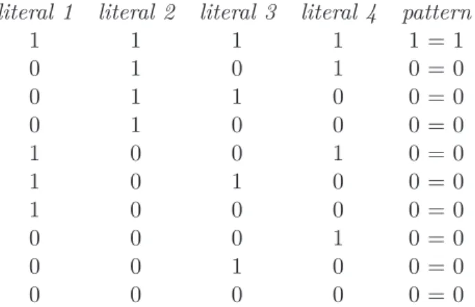
Lemma 1. An equivalence between indicators has exactly 10 valid valuations. Proof: Such an equivalence eq _{, I}a,b ≡ Ic,d is satisfied only when it matches one

of the 2 patterns 1 = 1 or 0 = 0: due to the fact that 0 is an absorbing value for ∧, these patterns correspond to the 10 valuations shown in Table 1 for the literals

involved in the indicators (with obvious notation). Any other valuation2 _{does not}

match anyone of the 2 previous patterns and will lead to the truth value 0 for the

equivalence eq. ✷

literal 1 literal 2 literal 3 literal 4 pattern

1 1 1 1 1 = 1 0 1 0 1 0 = 0 0 1 1 0 0 = 0 0 1 0 0 0 = 0 1 0 0 1 0 = 0 1 0 1 0 0 = 0 1 0 0 0 0 = 0 0 0 0 1 0 = 0 0 0 1 0 0 = 0 0 0 0 0 0 = 0

Table 1: 10 valid valuations for an equivalence between indicators

Proposition 1. The truth table of a logical proportion has 6 and only 6 valuations with truth value 1.

Proof: Since a logical proportion T is the conjunction eq1∧eq2of 2 equalities between

indicators, with eq1 Ó= eq2, it appears from Lemma 1 that T has a maximum of 10

valid valuations and a minimum of 4 valid valuations. Let us start from eq1, having 10 valid valuations which are candidate to validate T . Obviously, adding eq2 to eq1

will reduce the number of valid valuations for T . Let us assume eq2 differs from eq1

with only one literal (or negation operator). This is then a degenerated proportion. Without loss of generality, we can consider that the difference between eq1 and eq2

occurs on the first literal meaning eq1 is a ∧ l2≡ l3∧ l4 and eq2 is a ∧ l2≡ l3∧ l4 or

vice versa. It is then quite clear that the first valuation 1111 valid for eq1 is not valid

any more for T . It remains 9 candidates valuations. Finally any valuation starting with 01 is not valid any more and we have 3 such valuations. All the 6 remaining valuations are still valid for T . Which ends the proof when the 2 equalities differ from one negation (i.e. one literal). Now when they differ from 2 literals, two cases have to be considered:

2_{The only valuations considered in this paper pertain to 4-tuples of variables. In practice, a}

Boolean valuation v will be denoted by the values v(a)v(b)v(c)v(d) without any blank space, e.g., 0100 is short for v(a) = 0, v(b) = 1, v(c) = 0, v(d) = 0.

• either the 2 literals where eq1 differs from eq2 are on the same side of an

equivalence i.e. eq2 is l′1∧ l′2 ≡ l3∧ l4 (degenerated proportion)

• or they are on different side i.e. eq2 is l′1∧ l2 ≡ l′3∧ l4.

In the first case, the valuations 1111, 0010, 0001 and 0000 are not valid any more, but all other ones remain valid. In the second case, the valuations 0100, 0110, 1001 and 0001 are not valid anymore, but all the other ones remain valid. We are done for the case of 2 differences. When they differ from 3 literals, let us suppose l4

appears in both equivalence, the valuations 1001, 0101, 0010 and 0000 are not valid anymore and we stick with the 6 remaining ones. In the case where all the literals are different, obviously the 4 valuations containing only one occurrence of 1 are not valid anymore because they lead to an invalid pattern 0=1 or 1=0 for eq2. And we

have exactly 4 such valuations. It remains 6 valid valuations. ✷ Note that the negation of a logical proportion is not a logical proportion since such a negation has 10 valuations leading to true in its table. Besides, the 120 logical proportions are all distinct as shown below with the help of the following lemma. Lemma 2. Two equivalences between indicators have the same truth table iff they are identical.

Proof: It is sufficient to show that if 2 equalities eq1 and eq2 have the same truth

table, then they are syntactically identical. In other terms, we have to prove that

eq1 ≡ eq2 implies eq1 =Id eq2. Without loss of generality, let us assume that eq1 contains a but eq2 contains a. Considering the unique valuation v such that v(eq1) = 1 with the pattern 1 = 1, v is such that v(a) = 1. By hypothesis, v(eq2) = 1

but in that case with the pattern 0 = 0 since v(a) = 0. Let us now modify v into v′

such that v′_{(a) = v(a) = 0, v}′_{(c) = v(c), v}′_{(d) = v(d) and v}′_{(b) = v(b). Obviously v}′

does not validate eq1 but validates eq2 which contradicts the hypothesis. ✷

Proposition 2. The truth tables of the 120 proportions are all distinct.

Proof: We are going to show that, when 2 proportions T , eq1∧eq2and T′ , eq1′∧eq2′

have the same truth table, they are syntactically identical (up to a permutation of the 2 equalities). In other words, T ≡ T′ _{implies T =}

Id T′. Starting from T ≡ T′,

it amounts to show that if eq1 is syntactically different from eq′1, eq1 is syntactically

equal to eq′

2. This will complete the proof as a similar reasoning will show that eq2

is, in the same context, syntactically equal to eq′ 1.

In fact, if eq1 is syntactically different from eq′1, we can assume for instance

the unique valuation σ, validating T and T′_{, such that σ(eq}

1) = 1 with the pattern

1 = 1. Necessarily, this valuation σ is such that σ(a) = 1. By hypothesis, σ(eq′ 1) = 1

but in that case with the pattern 0 = 0 since σ(a) = 0. Let us now modify σ into σ′

such that σ′_{(a) = σ(a) = 0, σ}′_{(c) = σ(c), σ}′_{(d) = σ(d) and σ}′_{(b) = σ(b). Obviously} σ′_{(T ) = σ}′_(eq

1) = 0 but σ′(eq1) = 1 still following the pattern 0 = 0. The only

option for having σ(T ) = σ(T′_{) = 0 is thus to have σ}′_(eq′

2) = 0 which means a

belongs to eq′

2. Continuing the same reasoning, we show that eq1 =Id eq2′ and we

infer that if eq1Ó= eq1′, necessarily eq1 =Ideq2. ✷

Combined with the fact that there are C₁₆6 = 8008 truth tables with 16 lines, this result makes logical proportions quite rare in the world of quaternary Boolean formulas.

An exhaustive investigation of the whole set of logical proportions with respect to various other properties has been done in [19, 22, 21]. In the next subsection, we focus on one of these properties which allows us to characterize a small subset of remarkable proportions.

2.5 Code independency

Just as a numerical proportion holds independently of the base used for encoding numbers, or of the system of units representing the quantities at hand, it seems desirable that a logical proportion should be independent of the way we encode items in terms of the truth or the falsity of features. It means that the formula defining a proportion T should be valid when we switch 0 to 1 and 1 to 0. The formal expression of this property, that we call code independency, writes:

T (a, b, c, d) → T (a, b, c, d)

Surprisingly, this property highlights the fact once more that a single equivalence would not lead to a satisfactory definition for a logical proportion. Indeed, a unique equivalence between indicators, denoted l1∧ l2 ≡ l3∧ l4, where the li’s are literals

does not satisfy code independency, as explained now. If we consider a valuation v such that v(l1) = v(l2) = v(l3) = 0 and v(l4) = 1, obviously v makes the equivalence

valid since v(l1 ∧ l2) = v(l3∧ l4) = 0. But when we switch 0 to 1 and 1 to 0, it

appears that the new valuation v′_{such that v}′_(l

1) = v′(l2) = v′(l3) = 1 and v′(l4) = 0

does not validate the equivalence anymore. This shows that one equivalence is not enough if we are interested in “code independency”. We have to consider at least 2 equivalences to capture this behavior. For instance, (a ∧ b ≡ c ∧ d) ∧ (a ∧ b ≡ c ∧ d) clearly satisfies code independency.

Unfortunately, being built as the conjunction of two equivalences is not a suffi-cient condition for code independency, and many logical proportions do not satisfy it. We have the following result:

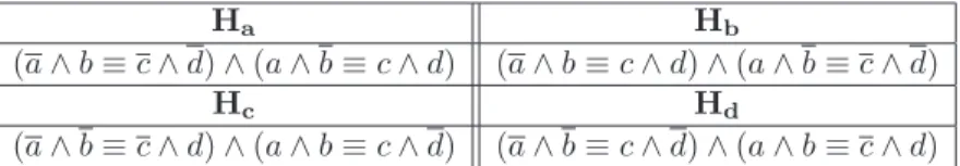
Proposition 3. There are exactly 8 proportions satisfying the code independency property: the 4 homogeneous proportions A, R, P, I, and 4 hybrid proportions (shown in Table 2).

Proof: In fact, the code independency property implies a complete equivalence: T (a, b, c, d) ↔ T (a, b, c, d)

Since both T (a, b, c, d) and T (a, b, c, d) are logical proportions, Proposition 2 tells us that the 2 proportions should be identical up to a permutation of the 2 equalities. This exactly means that the second equivalence is obtained from the first one by negating all the variables. Since we have 4 × 4 equalities between indicators, we can build exactly 16/2 = 8 proportions satisfying code independency property: each time we choose an equivalence, we use it and its negated form to build up a suitable proportion. Since A, R, P, I are built this way, they satisfy code independency. ✷

Ha Hb

(a ∧ b ≡ c ∧ d) ∧ (a ∧ b ≡ c ∧ d) (a ∧ b ≡ c ∧ d) ∧ (a ∧ b ≡ c ∧ d)

Hc Hd

(a ∧ b ≡ c ∧ d) ∧ (a ∧ b ≡ c ∧ d) (a ∧ b ≡ c ∧ d) ∧ (a ∧ b ≡ c ∧ d)

Table 2: The 4 hybrid proportions satisfying code independency

As a consequence of this result, this set of 8 proportions stand out of the whole set of 120 proportions. This set of proportions is clearly divided in 2 subsets: the 4 homogeneous proportions on one hand, and the 4 remaining ones, that we call

heterogeneous proportions, on the other hand. In the next two sections, we first

investigate the 4 homogeneous proportions through the angle of a list of meaningful properties, as well as their interrelationships, and their extensions to multiple-valued settings. After which, we shall move to the study of the 4 heterogeneous proportions in Section 5.

3

The 4 homogeneous proportions

We investigate now the 4 homogeneous proportions A, R, P, I from a semantical point of view. When considered as Boolean formulas, their semantics is given via their

truth tables (which have 24_{= 16 lines since these proportions involve 4 variables).}

3.1 Boolean truth tables

Starting from their syntactic expressions, it is an easy game to build up the truth tables of proportions A, R, P, I: they are exhibited in Table 3, where only the valu-ations leading to the truth value 1, are shown. This means that all the other ones lead to the truth value 0. As expected, only 6 valuations among 16 in the tables lead to a truth value 1. We also observe that there are only 8 distinct valuations that appear in Table 3. This emphasizes their collective coherence as the whole class of homogeneous proportions. Moreover, they go by pairs where 0 and 1 are exchanged, thus pointing out their “code independency”.

A R P I 0 0 0 0 0 0 0 0 0 0 0 0 1 1 0 0 1 1 1 1 1 1 1 1 1 1 1 1 0 0 1 1 0 0 1 1 0 0 1 1 1 0 0 1 1 0 0 1 1 1 0 0 1 1 0 0 0 1 1 0 0 1 1 0 0 1 0 1 0 1 1 0 0 1 0 1 0 1 0 1 1 0 1 0 1 0 0 1 1 0 1 0 1 0 1 0

Table 3: Analogy, Reverse analogy, Paralogy, Inverse paralogy truth tables It is interesting to take a closer look at the truth tables of the four homoge-neous proportions. First, one can observe in Table 3, that 8 possible valuations for (a, b, c, d) never appear among the patterns that make A, R, P , or I true: these 8 val-uations are of the form xxxy, xxyx, xyxx, or yxxx with x Ó= y and (x, y) ∈ {0, 1}2_.

As can be seen, it corresponds to situations where a = b and c Ó= d, or a Ó= b and c = d, i.e., similarity holds between the components of one of the pairs, and dissimilarity holds in the other pair. Moreover, the truth table of each of the four homogeneous proportions, is built in the same manner:

1. 2 lines of the table correspond to the characteristic pattern of the proportion; namely the two lines where one of the two equivalences in its definition holds true under the form 1 ≡ 1 (rather than 0 ≡ 0). Thus,

• A is characterized by the pattern xyxy (corresponding to valuations 1010 and 0101), i.e. we have the same difference between a and b as between

c and d;

• R is characterized by the pattern xyyx (corresponding to valuations 1001 and 0110), i.e., the differences between a and b and between c and d are

in opposite directions;

• P is characterized by the pattern xxxx (corresponding to valuations 1111 and 0000), i.e., what a and b have in common, c and d have it also; • I is characterized by the pattern xxyy (corresponding to valuations 1100

and 0011), i.e. what a and b have in common, c and d do not have it, and conversely.

2. the 4 other lines of the truth table of an homogeneous proportion T are gen-erated by the characteristic patterns of the two other proportions that are not opposed to T (in the sense that A and R are opposed, as well as P and I). For these four lines, the proportion holds true since its expression reduces to (0 ≡ 0) ∧ (0 ≡ 0).

Thus, the six lines of the truth table of A that makes it true are induced by the characteristic patterns of A, P , and I3_{, the six valuations that makes P true are}

induced by the characteristic patterns of P , A, and R, and so on for R and I.

3.2 Relevant properties

Before going deeper in the investigation, remember that the Boolean analogical proportion is supposed to be, in a Boolean setting, the counterpart of the classical numerical proportions. Then, it is interesting to consider Boolean counterparts of the properties satisfied by the numerical proportions, other than code independency. We list these properties below (with T denoting a logical proportion).

• Full identity: A numerical proportion holds when all the numbers are equal, i.e., a = b = c = d, which logically translates into

T (a, a, a, a)

• Reflexivity: A numerical proportion holds between (a, b) and (a, b) which log-ically translates into

T (a, b, a, b)

Obviously, reflexivity entails full identity.

3_{The measure of analogical dissimilarity introduced in [13] is 0 for the valuations corresponding}

to the characteristic patterns of A, P , and I, maximal for the valuations corresponding to the characteristic patterns of R, and takes the same intermediary value for the 8 valuations characterized by one of the patterns xxxy, xxyx, xyxx, or yxxx.

• Sameness: A numerical proportion holds between (a, a) and (b, b), which logi-cally translates into

T (a, a, b, b)

Still, sameness entails full identity.

• symmetry : We can exchange the pair (a, b) with the pair (c, d) in the numerical proportion, which logically translates into

T (a, b, c, d) → T (c, d, a, b)

• Central (and extreme) permutation : This is a well known property of numer-ical proportions, which lognumer-ically translates into

T (a, b, c, d) → T (a, c, b, d) (central permutation)

and

T (a, b, c, d) → T (d, b, c, a) (extreme permutation)

• Transitivity: This property that holds for numerical proportions is logically stated as follows

T (a, b, c, d) ∧ T (c, d, e, f ) → T (a, b, e, f )

• Exchange-mirroring: The negation operator can play for Boolean values the role of an inverse operator for numbers. A numerical proportion holds between a pair (a, b) and the pair(b−1_{, a}−1_{), which logically translates into}

T (a, b, b, a)

• Semi-mirroring: Similarly it is worth to consider

T (a, b, a, b)

This property is not satisfied by numerical proportions. • Negation-compatibility: Similarly it is worth to consider

T (a, a, b, b)

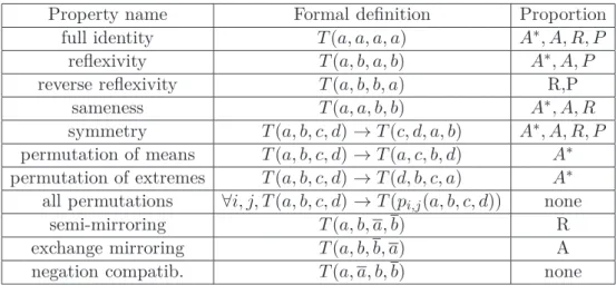
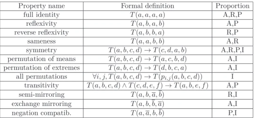
Property name Formal definition Proportion full identity T (a, a, a, a) A,R,P

reflexivity T (a, b, a, b) A,P reverse reflexivity T (a, b, b, a) R,P sameness T (a, a, b, b) A,R symmetry T (a, b, c, d) → T (c, d, a, b) A,R,P,I permutation of means T (a, b, c, d) → T (a, c, b, d) A,I permutation of extremes T (a, b, c, d) → T (d, b, c, a) A,I all permutations ∀i, j, T (a, b, c, d) → T (pi,j(a, b, c, d)) I

transitivity T (a, b, c, d) ∧ T (c, d, e, f ) → T (a, b, e, f ) A,P semi-mirroring T (a, b, a, b) R,I exchange mirroring T (a, b, b, a) A,I negation compatib. T (a, a, b, b) P,I

Table 4: Boolean properties of A, R, P, I

Investigating the homogeneous proportions with regard to the properties listed above can simply be done with an examination of the truth table of the target proportion. We summarize in Table 4 all the properties satisfied by A, R, P, I: the third col-umn enumerates the homogeneous proportions satisfying the property, respectively named and described in the 1st and 2nd columns.

Note that the 4 homogeneous proportions satisfy symmetry: T (a, b, c, d) = T (c, d, a, b), as well as many other properties. In particular, analogical proportion A enjoys properties that parallel properties of numerical proportions: full identity,

reflexivity, symmetry, central and extreme permutations, and transitivity.

One can also establish properties linking the homogeneous proportions, which are easily deducible from their definitions in terms of indicators.

Proposition 4.

A(a, b, c, d) ≡ R(a, b, d, c); A(a, b, c, d) ≡ P (a, d, c, b); A(a, b, c, d) ≡ I(a, d, c, b)

As can be seen, homogeneous proportions are strongly linked together. Especially

A, R, P are exchanged through simple permutation s; in that respect, I stands apart.

Besides, A, R, P, I are mutually exclusive, as a simple examination of their truth tables reveals that their intersection is empty.

Proposition 5. A(a, b, c, d) ∧ R(a, b, c, d) ∧ P (a, b, c, d) ∧ I(a, b, c, d) = ⊥

Lastly, having a closer look on the homogeneous proportions, we can easily build Table 5 which gives what T (a, b, c, d) ∧ T (c, d, e, f ) entails for the 4 homogeneous proportions.

chaining result transitivity A ∧ A A yes R ∧ R A no P ∧ P P yes I ∧ I P no A ∧ R R P ∧ I I

Table 5: Chaining properties for A, R, P, I

All these common properties explain why the homogeneous proportions stand out from the whole set of 120 logical proportions. It makes homogeneous proportions a worth considering Boolean counterpart of numerical proportions.

3.3 Characterization of homogeneous proportions by properties

Some subsets of the properties listed above are sufficient for characterizing one or more homogeneous proportions as unique among the 120 logical proportions. Let us start with the following result:

Proposition 6. • A, R, P are the unique proportions to satisfy full identity and

code independency.

• A is the only proportion to satisfy sameness (T (a, a, b, b)) and reflexivity

(T (a, b, a, b)).

• R is the only proportion to satisfy sameness and reverse reflexivity T (a, b, b, a). • P is the only proportion to satisfy reflexivity and reverse reflexivity.

• There is no proportion simultaneously satisfying sameness, reflexivity, and

re-verse reflexivity.

Proof: The first statement comes from Proposition 3 giving the 8 proportions

sat-isfying code independency, along with an immediate checking of the proportions syntactic form. For instance, Ha defined as (a ∧ b ≡ c ∧ d) ∧ (a ∧ b ≡ c ∧ d) is

defi-nitely not valid for valuation 0000. The same reasoning applies to all the proportions other than A, R, P .

This is an easy proof for the first 3 following statements since each property generates a set of 4 valid valuations (and two of them yield 6 valid valuations). For instance,

sameness (T (a, a, b, b) implies that valuations 1111, 0000, 0011, 1100 should be valid

and reflexivity (T (a, b, a, b)) implies that valuations 1111, 0000, 0101, 1010, which is the truth table of A.

Let us consider the last statement, having the simultaneous satisfaction of the 3 properties leads to a truth table where the 8 valuations 0000, 1111, 1010, 0101, 0110, 1001, 0011, 1100 are valid: then this cannot be the truth table of a logical

proportion. ✷

It is well known that a valid numerical proportion still holds when we exchange the extreme elements or the mean elements. And we have seen that A and I satisfy both of these permutations. In fact, there are 6 pairwise permutations of the 4 variables appearing in a proportion. So, the behavior of logical proportions w.r.t. these permutations is worth investigating. We denote the permutation of element

i and j by pi,j: for instance p2,3 is the mean permutation while p1,4 is the extreme

permutation. We can establish the following result:

Proposition 7. • A is the only proportion to satisfy reflexivity and to be stable

for p1,4 (or p2,3).

• A is the only proportion to satisfy sameness and to be stable for p1,4 (or p2,3).

• R is the only proportion to satisfy sameness and to be stable for p1,3 (or p2,4).

• R is the only proportion to satisfy reverse reflexivity and to be stable for p1,3 (or p2,4).

• P is the only proportion to satisfy reflexivity and to be stable for p1,2 (or p3,4).

• P is the only proportion to satisfy reverse reflexivity and to be stable for p1,2 (or p3,4).

• A and I are the only proportions to satisfy symmetry and to be stable for p1,4 (or p2,3).

• P and I are the only proportions to satisfy symmetry and to be stable for p1,2 (or p3,4).

• I is the unique logical proportion to satisfy the 6 permutations.

Proof: The proofs are quite similar for the 8 first statements. Let us give an example

for the first statement. reflexivity means that valuations 0000, 1111, 0011, 1100 have to be valid. Adding stability for p2,3 leads to add 0101 and 1010 as valid valuations.

Let us consider the last statement which is a bit more tricky. It is easy to check that these permutations induce a partition of the set of valuations into 5 classes, each of them being closed for these 6 permutations:

• the class {0000} and the class {1111} • the class {0111, 1011, 1101, 1110} • the class {1000, 0100, 0010, 0001}

• the class {0101, 1100, 0011, 1010, 1001, 0110}

Taking into account that a logical proportion is true for only 6 valuations (Proposi-tion 1), we only have 3 op(Proposi-tions:

- a proportion valid for {0000}, {1111} and {0111, 1011, 1101, 1110}, - or for {0000}, {1111} and {1000, 0100, 0010, 0001},

- or for {0101, 1100, 0011, 1010, 1001, 0110}.

It appears that the latter class is just the truth table of inverse paralogy. Lemma 3 that we shall prove below allows us to complete the proof. ✷

Lemma 3. A logical proportion cannot satisfies the class of valuation

{0111, 1011, 1101, 1110} or the class {1000, 0100, 0010, 0001}.

Proof: It is enough to show that this is the case for an equivalence between

indica-tors. So let us consider such an equivalence l1∧l2 ≡ l3∧l4. If this equivalence is valid

for {0111, 1011}, it means that its truth value does not change when we switch the truth value of the 2 first literals from 0 to 1: there are only 2 indicators for a and b satisfying this requirement: a ∧ b and a ∧ b. On top of that, if this equivalence is still valid for {1101, 1110}, it means that its truth value does not change when we switch the truth value of the 2 last literals from 0 to 1: there are only 2 indicators for c and

d satisfying this requirement: c ∧ d and c ∧ d. Then the equivalence l1∧ l2 ≡ l3∧ l4

is just a ∧ b ≡ c ∧ d, a ∧ b ≡ c ∧ d, a ∧ b ≡ c ∧ d or a ∧ b ≡ c ∧ d. None of these equivalences satisfies the whole class {0111, 1011, 1101, 1110}. The same reasoning

applies for the other class. ✷

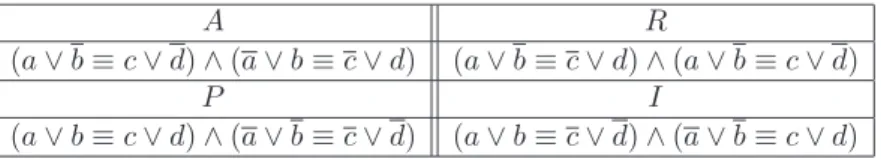
We summarize the results of this subsection by a pair of properties characterizing a subset of homogeneous proportions, in Table 6 and Table 7. An empty cell means that the corresponding properties do not characterize any subset of homogeneous proportion. For instance, the diagonal cells are all empty because an homogeneous proportion cannot be characterized with only one property.

full identity code indep. symmetry sameness reflexivity rev. reflexivity full identity A, R, P code indep. A, R, P A, R, P, I A, R A, P R, P symmetry A, R, P, I A, R R, P sameness A, R A, R A R reflexivity A, P A P rev. reflexivity R, P R, P R P

Table 6: Characteristic properties of A, R, P, I

p1,2 p1,3 p1,4 p2,3 p2,4 p3,4

sameness R A A R reflexivity P A A P rev. reflexivity P R R P symmetry P, I A, I A, I P, I

Table 7: Characteristic properties of A, R, P, I w.r.t. permutations

To conclude this section, we establish a result which shows how singular I is among the set of homogeneous proportions.

Proposition 8.

• A logical proportion satisfying 2 properties among semi-mirroring,

negation-compatibility and exchange-mirroring satisfies the remaining one, and is unique. This is the inverse paralogy I.

• A logical proportion stable for 4 permutations is stable for the 2 remaining

ones and is unique. This is the inverse paralogy I.

Proof: Considering the first statement, let us choose for instance semi-mirroring

and negation-compatibility. First of all, we can observe that, for a proportion T to satisfy semi-mirroring, means the 4 valuations 1010, 1001, 0110, 0101 are valid. For negation-compatibility to be satisfied, the 4 valuations 1100, 0011, 1001, 0110 should be valid. Then the truth table of a proportion satisfying both properties should contains all these valuations i.e. 1010, 1001, 0110, 0101, 1100, 0011. Thanks to Proposition 1, this is the truth table of inverse paralogy I. A similar reason-ing applies for the other cases. Regardreason-ing the second statement, let us consider a proportion stable for 4 pairwise permutations: since such pairwise permutations generate the full group of permutations of 4 elements, it means this proportion is stable for any permutations. We can consider 2 cases:

- either such a proportion is valid for a valuation having an even number of 0 and other than 0000 and 1111. We can consider this is 0110 for instance. The stability leads to have 0011, 0110, 0101, 1001, 1010 valid as well: this is the truth table for i.

- or such a proportion does not have a valid valuation with an even number of 0 other than 0000 and 1111. It means there is a valid valuation with an odd number of 0 like 1000. In that case, the stability w.r.t. the permutations leads to have 1000, 0100, 0010, 0001 as valid valuations, which is not possible thanks to

Lemma 3. ✷

3.4 Equation solving

The idea of proportion is closely related to the idea of extrapolation, i.e. to guess/-compute a new value on the ground of existing values. In the case of geometrical proportions, this leads to the well known “rule of three” where, knowing that a

b = c x

holds, allows us to compute the value of x from a, b, c. In the Boolean setting, if for some reason it is believed or known that a logical proportion holds between 4 binary items, 3 of them being known, then one may try to infer the value of the 4th one, at least when this extrapolation leads to a unique value. For a proportion T , there are exactly 6 valuations v such that:

In our context, the problem can be stated as follows. Given a logical proportion T and a valuation v such that v(a), v(b), v(c) are known, does it exist a Boolean value

x such that v(T (a, b, c, d)) = 1 when v(d) = x, and in that case, is this value unique?

We will refer to this problem as “the equation solving problem”, and for the sake of simplicity, a propositional variable a is denoted as its truth value v(a), and we use the equational notation T (a, b, c, x) = 1, where x ∈ {0, 1} is unknown. First of all, it is easy to see that there are always cases where the equation has no solution. Indeed, the triple a, b, c may take 23 = 8 values, while any proportion T is true only for 6 distinct valuations, leaving at least 2 cases with no solution. For instance, when we deal with analogy A, the equations A(1, 0, 0, x) and A(0, 1, 1, x) have no solution. We have the following results:

Proposition 9.

The analogical equation A(a, b, c, x) is solvable iff (a ≡ b) ∨ (a ≡ c) holds. In that case, the unique solution is x = a ≡ (b ≡ c).

The reverse analogical equation R(a, b, c, x) is solvable iff (b ≡ a) ∨ (b ≡ c) holds. In that case, the unique solution is x = b ≡ (a ≡ c).

The paralogical equation P (a, b, c, x) is solvable iff (c ≡ b) ∨ (c ≡ a) holds.

In each of the three above cases, when it exists, the unique solution is given by x = c ≡ (a ≡ b), i.e. x = a ≡ b ≡ c.

The inverse paralogical equation I(a, b, c, x) is solvable iff (a Ó≡ b) ∨ (b Ó≡ c) holds. In that case, the unique solution is x = c Ó≡ (a Ó≡ b).

Proof: By immediate investigation of the truth tables. ✷

The anthropologist, linguist and computer scientist Sheldon Klein [9, 10] was the first to propose to solve analogical equations of the form A(a, b, c, x) = 1, where

x is unknown, as x = c ≡ (a ≡ b), without however providing an explicit definition

for A(a, b, c, d), nor distinguishing between A, R, and P . As we can see, the first 3 homogeneous proportions A, R, P behave similarly. Still, their conditions of equation solvability differ. Moreover, it can be checked that at least 2 of these proportions are always simultaneously solvable. Besides, when they are solvable, there is a common expression that yields the solution.

3.5 Alternative writings for homogeneous proportions

When sticking to the Boolean setting, we can use standard equivalences to get alternative writings for A, R, P, I. First of all, using the De Morgan’s laws and the fact that p ≡ q is equivalent to p ≡ q, we get definitions where the internal ∧ are

replaced with ∨ as shown in Table 8. It means that, in a Boolean setting, indicators involving ∨ are a perfect replacement for indicators using ∧.

A R

(a ∨ b ≡ c ∨ d) ∧ (a ∨ b ≡ c ∨ d) (a ∨ b ≡ c ∨ d) ∧ (a ∨ b ≡ c ∨ d)

P I

(a ∨ b ≡ c ∨ d) ∧ (a ∨ b ≡ c ∨ d) (a ∨ b ≡ c ∨ d) ∧ (a ∨ b ≡ c ∨ d)

Table 8: A, R, P, I definitions with ∨ operator

A more interesting option is to start from the definition of P with indicators (a ∧ b ≡ c ∧ d) ∧ (a ∧ b ≡ c ∧ d) (P )

and to use again De Morgan’s laws to rewrite the second equivalence. This leads to a definition of P without any negation that we denote P∗_:

(a ∧ b ≡ c ∧ d) ∧ (a ∨ b ≡ c ∨ d) (P∗₎

Then, considering the link between A and P established in Proposition 4, namely

A(a, b, c, d) ≡ P (a, d, c, b), it comes another definition for A, without any negation

operator:

(a ∧ d ≡ b ∧ c) ∧ (a ∨ d ≡ b ∨ c) (A∗₎

It is noticeable that this latter new definition exactly corresponds to what the psy-chologist Jean Piaget [15], called logical proportion! However, strangely enough, he has not developed their study nor pointed out their link with analogy.

Thus, since a and d are the extreme variables, b and c the mean variables, the analogical proportion A(a, b, c, d) can be read as “the conjunction (resp. disjunction) of the extremes is equivalent to the conjunction (resp. disjunction) of the means”.

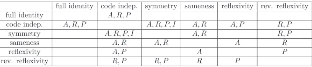
Considering the link between A, R, P, I coming from Proposition 4, we can finally get alternative writing denoted A∗_{, R}∗_{, P}∗ _{and I}∗ _{that are shown in Table 9.}

A∗ _R∗

(a ∧ d ≡ b ∧ c) ∧ (a ∨ d ≡ b ∨ c) (a ∧ c ≡ b ∧ d) ∧ (a ∨ c ≡ b ∨ d)

P∗ _I∗

(a ∧ b ≡ c ∧ d) ∧ (a ∨ b ≡ c ∨ d) (a ∧ b ≡ c ∧ d) ∧ (a ∨ b ≡ c ∨ d)

Since, in the Boolean setting, the equivalence T (a, b, c, d) ≡ T∗_{(a, b, c, d) holds}

(where T denotes any homogeneous proportion among A, R, P, I), one could consider

T∗ _{as an alternative writing for T . It is interesting to note that this approach}

leads to rewrite A, R, P without any negation. We have to be aware that these equivalences, leading to alternative writings, are not necessarily valid outside the Boolean framework.

4

Homogeneous proportions:

multiple-valued semantics

Ultimately, logical proportions, and in particular the homogeneous ones, could be used for practical applications where we have to deal with missing information or features whose satisfaction is a matter of degree. To cover such situations, exten-sions of the Boolean interpretation to multiple-valued logics (3-valued at least) is necessary. A formal way to cope with these situations is to extend the Boolean framework to a multiple-valued one by introducing truth values belonging to [0, 1]. We should carefully distinguish between three cases:

• when feature satisfaction is a matter of degree instead of being binary, i.e., the truth value of a given feature may be an intermediate value between 0 and 1. • when a feature does not make sense for a given item, i.e., the feature is non

applicable to it.

• when information about some features is missing, i.e., we have no clue about the truth value of some features for some items, and the corresponding truth value is not known, i.e., unknown.

At this stage, two questions arise:

1. in a given model, what are the valuations that correspond to a “perfect” pro-portion of a given type (i.e., having 1 as truth value)? For instance, does

T (a, a, a, a) postulate still have to be satisfied by A, R, P , or can we consider

models where A(u, u, u, u) = u, u being a truth value distinct from 0 and 1? 2. are there valuations that could be regarded as “imperfect” proportions of a

given type (i.e., with a truth value distinct from 0 and 1) and in that case, what is their truth value?

We investigate these issues in the following subsections keeping in mind an essential principle: whatever the way we define the truth values, the Boolean model should be the limit case of our models when restricted to Boolean valuations.

4.1 Semantics for gradual features

When the satisfaction of features may be a matter of degree, we have to consider that the truth values belong to a linearly ordered scale L. The simplest case is when L = {0, α, 1}, with the ordering 0 < α < 1, which can be generalized into a finite chain L = {α0 = 0, α1, · · · , αn = 1} of ordered grades 0 < α1 < · · · < 1, or to an

infinite chain using the real interval [0, 1]. A proposal for extending A in such cases has been advocated in [18]. It takes its source in the initial definition

A(a, b, c, d) = (a ∧ ¯b ≡ c ∧ ¯d) ∧ (¯a ∧ b ≡ ¯c ∧ d),

where now

• i) the central ∧ is taken as equal to min;

• ii) s ≡ t is taken as min(s →Lt, t →Ls) where →Lis Łukasiewicz implication,

defined by s →L t = min(1, 1 − s + t), for L = [0, 1] (in the discrete cases,

we take α = 1/2 and αi = i/n), and thus s ≡ t = 1 − |s − t| ; note that

s ≡ t = (1 − s) ≡ (1 − t);

• iii) s ∧ ¯t = max(0, s − t) = 1 − (s →Lt), i.e., ∧¯is understood as expressing a

bounded difference. Note that this choice preserves A(a, b, c, d) = A(¯a, ¯b, ¯c, ¯d)

for the involutive negation ¯x = 1 − x.

The resulting expression for A(a, b, c, d) is given in Table 10. Then, we under-stand the truth value of A(a, b, c, d) as the extent to which the truth values a, b, c, d makes an analogical proportion. For instance, in such a graded model, the truth value of A(0.9, 1, 1, 1) = 0.9, which fits the intuition. It can be checked that the semantics of A(a, b, c, d) thus defined in the graded case, reduces to the previous definition when restricted to the Boolean case.

It is interesting to study in what cases A(a, b, c, d) = 1 (and in what cases

A(a, b, c, d) = 0). Then it is clear that A(a, b, c, d) = 1 when a − b = c − d. When a, b, c, d ∈ {0, α = 1/2, 1}, it yields the 19 following patterns 1111; 0000; αααα;

1010; 0101; 1α1α; α1α1; 0α0α; α0α0; 1100; 0011; 11αα; αα11; αα00; 00αα; 1αα0; 0αα1; α10α; α01α.

This means that A(a, b, c, d) = 1 when the change from a to b has the same direction and the same intensity as the change from c to d. However, the last 4 patterns show that there is no need to have a = b and a = c while these conditions hold for the 15 first patterns, which are all of the form xyxy, xxyy, or xxxx. In contrast, note that the last 4 patterns exhibit 3 distinct values.

A(a, b, c, d) = 0 when a − b = 1 and c ≤ d, or b − a = 1 and d ≤ c, or a ≤ b and c − d = 1, or b ≤ a and d − c = 1. It means the 22 following patterns in the 3-valued

A(a, b, c, d) =

1− | (a − b) − (c − d) | if a ≥ b and c ≥ d, or a ≤ b and c ≤ d 1 − max(| a − b |,| c − d |) if a ≤ b and c ≥ d, or a ≥ b and c ≤ d

R(a, b, c, d) = A(a, b, d, c) P∗_{(a, b, c, d) =}

min(1 − |max(a, b) − max(c, d)|, 1 − |min(a, b) − min(c, d)|)

Table 10: Graded definitions for A, R, P∗

case: 1110; 1101; 1011; 0111; 0001; 0010; 0100; 1000; 1001; 0110; 10αα; 01αα; αα10;

αα01; 100α; 011α; 10α1; α001; 0α10; 1α01; 01α0; α110. Thus, A(a, b, c, d) = 0 when

one change inside the pairs (a, b) and (c, d) is maximal, while the other pair shows no change or a change in the opposite direction.

Using L = {0, α, 1}, A(a, b, c, d) = α for 81 - 19 - 22 = 40 distinct patterns.

In [18], the graded extension of R(a, b, c, d) is defined by permuting c and d in the definition of A, according to Proposition 4. But the extension of the paralogy is no longer obtained by permuting b and d in the definition of A (as Proposition 4 would suggest). In fact, the paralogical proportion is defined directly from P∗

(thus changing ¯a ∧ ¯b ≡ ¯c ∧ ¯d into a ∨ b ≡ c ∨ d), and taking ∧ = min, ∨ = max,

and s ≡ t = 1 − |s − t|, we obtain the definition in Table 10. If we now exchange b and d (using Proposition 4 again) in this definition, we get the graded version of A∗

(which is no longer equivalent to A), namely

A∗_{(a, b, c, d) = min(1 − |max(a, d) − max(b, c)|, 1 − |min(a, d) − min(b, c)|)}

This is the direct counterpart of the definition without negation of the analogical pro-portion in the Boolean case. This alternative extension still preserves A∗_{(a, b, c, d) =} A∗_{(¯a, ¯b, ¯c, ¯d) for the involutive negation ¯x = 1−x. It can be checked that A}∗_{(a, b, c, d)}

= 1 only for the 15 patterns with at most two distinct values (for which A(a, b, c, d) = 1), while A∗_{(a, b, c, d) = α for the 4 other patterns for which A(a, b, c, d) = 1, namely}

for 1αα0; 0αα1; α10α; α01α. Besides, A∗_{(a, b, c, d) = 0 for only 18 among the 22}

patterns that make A(a, b, c, d) = 0. The 4 patterns for which A∗_{(a, b, c, d) = α}

(instead of 0) are 10αα; 01αα; αα10; αα01.

Thus, it appears that A∗_{(a, b, c, d) does not acknowledge as perfect the analogical}

proportion patterns where the amount of change between a and b is the same as between c and d and has the same direction, but where this change applies in different areas of the truth scale. Still, A∗_{(a, b, c, d) remains half-true in these cases, for}

L = {0, α, 1}. When L = [0, 1], it can be checked that A∗_{(a, b, c, d) ≥ 1/2 when} a − b = c − d; in particular, ∀a, b, A∗_{(a, b, a, b) = 1, which corresponds to the case}

where a = c and b = d. In the same spirit, if L = {0, α, 1} as well as for L = [0, 1],

A∗_{(a, b, c, d) = 0 when a change inside the pairs (a,b) and (c,d) is maximal, while the}

other pair shows a change in the opposite direction starting from 0 or 1. However,

A∗_{(1, 0, c, c) = min(c, 1−c) and A}∗_{takes the same value for the 7 other permutations}

of (1, 0, c, c) obtained by applying symmetry and/or central permutation.

As can be seen in Table 11, A∗ _{and A also coincide on some patterns having}

intermediary truth values, but diverge on others. Generally speaking, A∗_{is smoother}

than A in the sense that more patterns have intermediary truth values with A∗_than

with A. A A∗ A(1, 1, u, v) = 1 − |u − v| A∗_{(1, 1, u, v) = 1 − |u − v|} A(1, 0, u, v) = u − v if u ≥ v A∗_{(1, 0, u, v) = min(u, 1 − v)} = 0 if u ≤ v A(0, 1, u, v) = v − u if u ≤ v A∗_{(0, 1, u, v) = min(v, 1 − u)} = 0 if u ≥ v A(0, 0, u, v) = A(1, 1, u, v) A∗_{(0, 0, u, v) = A}∗_{(1, 1, u, v)}

Table 11: The two graded definitions of the analogical proportion in [0, 1]

Both A and A∗ _{continue to satisfy the symmetry property (as P, R, and P}∗_{, R}∗

with R∗_{(a, b, c, d) = A}∗_{(a, b, d, c) = P}∗_{(a, c, d, b)). However, only A}∗ _{still enjoys the} means permutation and the extremes permutation properties. This is no longer the case with A, as shown by the following counter-example.

A(0.8, 0.6, 1, 0.3) = 1− | (0.8 − 0.6) − (1 − 0.3) |= 1− | 0.2 − 0.7 |= 0.5 since

0.8 ≥ 0.6 and 1 ≥ 0.3, and A(0.8, 1, 0.6, 0.3) = 1 − max(| 0.8 − 1 |, | 0.6 − 0.3 |) = 1−max(0.2, 0.3) = 0.7 since 0.8 ≤ 1 and 0.6 ≥ 0.3.

But, as already mentioned, both A and A∗ _{continue to satisfy the code} inde-pendency property with respect to a = 1 − a. Some more Boolean properties that