HAL Id: hal-01882680
https://hal.archives-ouvertes.fr/hal-01882680
Submitted on 5 Jul 2019
HAL is a multi-disciplinary open access
archive for the deposit and dissemination of
sci-entific research documents, whether they are
pub-lished or not. The documents may come from
teaching and research institutions in France or
abroad, or from public or private research centers.
L’archive ouverte pluridisciplinaire HAL, est
destinée au dépôt et à la diffusion de documents
scientifiques de niveau recherche, publiés ou non,
émanant des établissements d’enseignement et de
recherche français ou étrangers, des laboratoires
publics ou privés.
On the search for representative characteristics of PV
systems: Data collection and analysis of PV system
azimuth, tilt, capacity, yield and shading
Sven Killinger, David Lingfors, Yves-Marie Saint-Drenan, Panagiotis Moraitis,
Wilfried van Sark, Jamie Taylor, Nicholas Engerer, Jamie Bright
To cite this version:
Sven Killinger, David Lingfors, Yves-Marie Saint-Drenan, Panagiotis Moraitis, Wilfried van Sark, et
al.. On the search for representative characteristics of PV systems: Data collection and analysis of PV
system azimuth, tilt, capacity, yield and shading. Solar Energy, Elsevier, 2018, 173, pp.1087 - 1106.
�10.1016/j.solener.2018.08.051�. �hal-01882680�
See discussions, stats, and author profiles for this publication at: https://www.researchgate.net/publication/327279306
On the search for representative characteristics of PV systems Data collection
and analysis of PV system azimuth, tilt, capacity, yield and shading
Article in Solar Energy · August 2018
DOI: 10.1016/j.solener.2018.08.051 CITATIONS 8 READS 266 8 authors, including:
Some of the authors of this publication are also working on these related projects:
localization and parameterization of existing PV systems using artificial neural networks and image recognition techniquesView project
Solar charge 2020View project Sven Killinger
Fraunhofer Institute for Solar Energy Systems ISE 47PUBLICATIONS 174CITATIONS SEE PROFILE David Lingfors Uppsala University 33PUBLICATIONS 289CITATIONS SEE PROFILE Yves-Marie Saint-Drenan
MINES ParisTech, PSL Research University 36PUBLICATIONS 191CITATIONS SEE PROFILE Panagiotis Moraitis Utrecht University 14PUBLICATIONS 44CITATIONS SEE PROFILE
On the search for representative characteristics of PV systems: Data
collection and analysis of PV system azimuth, tilt, capacity, yield and
shading
Sven Killingera,b, David Lingforsc, Yves-Marie Saint-Drenand, Panagiotis Moraitise, Wilfried van Sarke, Jamie Taylorf, Nicholas A. Engerera,2,∗∗, Jamie M. Brighta,∗
aFenner School of Environment and Society, The Australian National University, 2601 Canberra, Australia bFraunhofer Institute for Solar Energy Systems ISE, 79100 Freiburg, Germany
cDepartment of Engineering Sciences, Uppsala University, Lgerhyddsvgen 1, 752 37 Uppsala, Sweden
dMINES ParisTech, PSL Research University, O.I.E. Centre Observation, Impacts, Energy, 06904 Sophia Antipolis, France eCopernicus Institute of Sustainable Development, Utrecht University, 3508 TC Utrecht, The Netherlands
fSheffield Solar, University of Sheffield, Hicks Building, Hounsfield Road, Sheffield S3 7RH, UK
Abstract
Knowledge of PV system characteristics is needed in different regional PV modelling approaches. It is the aim of this paper to provide that knowledge by a twofold method that focuses on (1) metadata (tilt and azimuth of modules, installed capacity and specific annual yield) as well as (2) the impact of shading.
Metadata from 2,802,797 PV systems located in Europe, USA, Japan and Australia, representing a total capacity of 59 GWp (14.8% of installed capacity worldwide), is analysed. Visually striking interdependencies of the installed capacity and the geographic location to the other parameters tilt, azimuth and specific annual yield motivated a clustering on a country level and between systems sizes. For an eased future utilisation of the analysed metadata, each parameter in a cluster was approximated by a distribution function. Results show strong characteristics unique to each cluster, however, there are some commonalities across all clusters.
Mean tilt values were reported in a range between 16.1◦ (Australia) and 35.6◦ (Belgium), average specific
annual yield values occur between 786 kWh/kWp (Denmark) and 1,426 kWh/kWp (USA South). The region with smallest median capacity was the UK (2.94 kWp) and the largest was Germany (8.96 kWp). Almost all countries had a mean azimuth angle facing the equator.
PV system shading was considered by deriving viewsheds for ≈ 48,000 buildings in Uppsala, Sweden (all ranges of solar angles were explored). From these viewsheds, two empirical equations were derived related to irradiance losses on roofs due to shading. The first expresses the loss of beam irradiance as a function of the solar elevation angle. The second determines the view factor as a function of the roof tilt including the impact from shading and can be used to estimate the losses of diffuse and reflected irradiance.
1. Introduction 1
With 402.5 GW of installed photovoltaic (PV) 2
capacity globally (IEA,2018), the integration of the 3
large amounts of energy generated by the numerous 4
distributed solar power systems into the electricity 5
supply system is an issue ever gaining in impor-6
tance. Modelling of the power generated by those 7
decentralised solar systems is of utmost importance 8
for several issues ranging from energy trading to 9
network flow control. The estimation and forecast 10
of PV power is made difficult by the fact that only a 11
minority of systems continuously report their gen-12
eration and are publicly accessible. 13
Different strategies have been proposed to over-14
come the lack of reporting (e.g. upscaling
ap-15
proaches or power simulations based on satellite de-16
rived irradiance); an extensive literature overview is 17
provided inBright et al. (2017b). Within this
pa-18
per, the estimation of the aggregated power gen-19
erated in a given region by a fleet of unknown 20
PV systems is referred to as regional PV power 21
modelling. Knowledge of PV system characteris-22
tics is required in the different regional PV mod-23
elling approaches to reconstruct the missing power 24
measurements (Lorenz et al., 2011; Saint-Drenan
25
et al., 2016). Some studies assign simplified
as-26
sumptions of the PV system characteristics. This 27
can result in over-exaggerated grid impacts (Bright
28
et al.,2017a). Unfortunately in most cases,
charac-29
teristics from PV systems are either unknown or 30
∗Corresponding author ∗∗Co-corresponding author
Email addresses: nicholas.engerer@anu.edu.au (Nicholas A. Engerer), jamie.bright@anu.edu.au (Jamie M. Bright), jamiebright1@gmail.com (Jamie M. Bright)
only accessible for a small number of stakehold-31
ers (inverter manufacturers, monitoring solutions 32
providers, etc.). As a result, progress in the area 33
of regional PV power estimation or forecasting can 34
be considered sub-optimal as potential contributors 35
like universities or small companies are partially ex-36
cluded from access to larger datasets of measure-37
ments or metadata. This is still the case despite 38
grid integration of solar energy being considered a 39
strategic societal issue. Therefore, it is the aim of 40
this paper to offer any stakeholders the possibility 41
to develop activities on this research field by col-42
lecting, analysing and disseminating metadata on 43
millions of PV systems installed worldwide. To be-44
gin, we must establish which metadata are the most 45
important. 46
Saint-Drenan (2015) carried out a sensitivity
47
analysis and found that the four most influen-48
tial characteristics impacting PV output genera-49
tion are: (1) tilt angle and (2) azimuth angle of 50
PV modules, (3) installed capacity and (4) total ef-51
ficiency (represented herein as the specific annual 52
yield). Furthermore, (5) shading is of crucial in-53
fluence on the PV power generation but is not ac-54
cessible from PV system metadata. The impact
55
of shading can only be accessed with considerable 56
effort, e.g. simulations that consider digital eleva-57
tion models (DEM) including buildings, trees and 58
other obstacles, by analysing PV power profiles or 59
even weekly performance ratios (seePaulescu et al.
60
(2012);Freitas et al.(2015);Lingfors et al.(2018);
61
Tsafarakis et al. (2017) for further reading). Due
62
to its significant influence, a shading analysis com-63
plements the focus of this study. 64
These five identified characteristics are the cen-65
tral focus of this paper because of their general 66
importance for regional PV modelling approaches. 67
The overall aim of this paper is to achieve a full re-68
producibility of the five characteristics so that they 69
can be used in regional PV power modelling appli-70
cations such as nowcasting or forecasting, but also 71
in power simulations that are used for energy sys-72
tem analysis, studying the grid impact, defining the 73
PV power potential etc. 74
1.1. Related work 75
The relevant literature for this research has three 76
prominent categories: (1) metadata analysis with 77
intention to improve regional PV power simula-78
tions, (2) PV performance due to specific yield, and 79
(3) models that consider shading analysis. 80
Category 1: Examples of literature using meta-81
data to improve regional PV power simulations. 82
Schubert (2012) provides a useful guidebook for
83
the simulation of PV power that sketches impor-84
tant parts of the simulation chain and delivering 85
assumptions for characteristics. An overview of dif-86
ferent characteristics of tilt, azimuth, the module 87
and installation type are given together with sug-88
gested weights. However, these weights seem to be 89
assumptions with no datasets being cited as an em-90
pirical basis and so using these weights in PV sim-91
ulations raise questions of trust. 92
Datasets are used by Lorenz et al. (2011), who
93
evaluated the representativeness of a set of ref-94
erence PV systems to predict regional PV power 95
by analysing the orientation and module types of 96
≈ 8, 000 systems in Germany. The authors note 97
that their dataset seem to have a disproportionate 98
share of large PV systems and so do not fully rep-99
resent a larger portfolio. 100
The problem of poor representativeness was by-101
passed inSaint-Drenan(2015);Saint-Drenan et al.
102
(2017) by feeding a PV model with metadata
statis-103
tics from a larger sample of PV systems as opposed 104
to a smaller and unrepresentative subset. They de-105
rived joint probabilities of azimuth and tilt from 106
35,000 systems and clustered them by their sys-107
tem size and geographic location. These empiric 108
distributions where then used to estimate the char-109
acteristics of all 1,500,000 PV systems installed in 110
Germany at that time. Saint-Drenan et al. (2018)
111
complemented their earlier research by reproduc-112
ing it for more European countries using statistical 113
distributions from 35,000 PV systems in Germany 114
and 20,000 in France. This demonstrates the sig-115
nificant potential of generating representative sta-116
tistical distributions with intended use in regional 117
PV power simulations. 118
K¨uhnert(2016, pp. 80-85) followed a similar
ap-119
proach and derived statistical distributions for tilt 120
and azimuth from ≈ 1,300 PV systems in Germany. 121
Based on this portfolio, the author evaluated the 122
representativeness should PV systems be clustered 123
into different geographic regions and system sizes. 124
The authors quantitatively derived recommenda-125
tions between the two extremes of (1) a portfolio 126
covering all PV systems and (2) a high number of 127
subclasses with a very small number of PV systems. 128
From this, we observe that there must be a well 129
considered clustering approach in order to derive 130
representative subclasses. 131
Killinger et al. (2017c) detailed a regional PV
132
power upscaling approach which estimated the 133
power of ≈ 2,000 target PV systems based on 45 134
continuously measured PV systems in Freiburg, 135
Germany. Whereas the azimuth and tilt of the 45 136
measured systems were known in their case, both 137
parameters were derived through a geographic in-138
formation system (GIS) based approach for the tar-139
get PV systems. 140
Furthermore,Pfenninger and Staffell (2016) use
141
PV power measurements and incorporate metadata 142
from 1,029 systems in 25 European countries to de-143
rive empirical correction factors for PV power sim-144
ulations. A comparison between the analysed tilt 145
and latitude showed an trend towards steeper an-146
gles at higher latitudes, indicating that metadata 147
might vary with the geographic location. 148
PV system metadata is thus used to successfully 149
improve regional PV power upscaling across Europe 150
in Pfenninger and Staffell (2016); Killinger et al.
151
(2017c); Saint-Drenan (2015); Saint-Drenan et al.
152
(2017,2018);K¨uhnert(2016). These works applied
153
information of azimuth, tilt, installed capacity and 154
the geographic location from PV systems to esti-155
mate the power output of a larger PV fleet for sim-156
ilar geographies and different countries. They stand 157
as an powerful and excellent example for how rep-158
resentative metadata distribution statistics can be 159
employed. It is these examples that guide the first 160
usage of our vast dataset towards deriving repre-161
sentative metadata distributions. 162
Category 2: Excerpts of literature that analyse 163
the performance of PV systems. Performance is
164
more complex than just tilt and azimuth as it is 165
inherently influenced by other components, such as 166
soiling and meteorology. 167
Nordmann et al.(2014) found a positive
correla-168
tion between specific annual yield and incoming ir-169
radiance, as well as an observed negative correlation 170
between system performance and ambient temper-171
ature. Their data was obtained via web-scraping of 172
Solar-Log (2,914 systems in the Netherlands, Ger-173
many, Belgium, France and Italy) and collected by 174
participants of the IEA task (>60,000 systems in 175
the USA). 176
Moraitis et al.(2015) observed an increasing yield
177
with decreasing latitude from ≈ 20,000 systems in 178
Netherlands, Germany, Belgium, France and Italy, 179
also achieved using web-scraping techniques. We 180
therefore expect to observe geographical differences 181
due to latitude and climate. 182
Taylor (2015) explored the generation of 4,369
183
distributed systems in the UK to derive the per-184
formance ratio and degradation rate. To allow re-185
producibility, the analysis of the performance ratio 186
was enriched by approximating it with distribution 187
functions. We intend to extend this style of analysis 188
to PV system metadata. 189
Leloux et al.(2012a) examined data from
residen-190
tial PV systems in Belgium; Leloux et al. (2012b)
191
focused on France. In Belgium, specific annual
192
yield was analysed for 158 systems in 2009 and 193
normalised by a factor which compared the incom-194
ing irradiance in this year to a 10 year average. 195
The mean value was 836 kWh/kWp. The same ap-196
proach led to a mean value of 1,163 kWh/kWp for 197
1,635 systems in 2010 in France. Weibull distribu-198
tions were used throughout both papers to approxi-199
mate the specific yield and performance indicators; 200
Weibull distributions were selected for visual simi-201
larity and not for robustness of fit — we aim to use a 202
more statistically rigorous approach to distribution 203
type selection. Furthermore, a relative distribution 204
was provided for combinations of tilt and azimuth. 205
Additionally, the installed capacity was analysed in 206
France, showing a high number of systems with 3 207
kWp or slightly less. The reason for this is due to 208
tax credits being denied for system sizes > 3kWp 209
and a strongly increased VAT for such system sizes 210
(Leloux et al., 2012b). The legal framework can
211
thus have a strong influence on characteristics of 212
PV systems. Further studies exist which analyse 213
the specific energy of PV systems. However, most 214
of these studies are limited to a particular region 215
and less of them propose a parametric approxima-216
tion of the data studied. 217
Category 3 — the impact of shading in many ar-218
ticles is only considered in a highly simplified man-219
ner, e.g. by setting irradiance values zero above 220
a certain solar zenith angle (Lingfors and Wid´en,
221
2016), restricting simulations and analyses to time
222
steps with certain solar zenith angles (Elsinga and
223
van Sark, 2015;Elsinga et al.,2017;Jamaly et al.,
224
2013; Killinger et al., 2016; Saint-Drenan et al.,
225
2017; Yang et al., 2014; Bright et al., 2015),
ap-226
plying constant losses (Mainzer et al., 2017) or as-227
suming a linear decrease in the PV power values 228
(Schubert, 2012). Several authors expect
improve-229
ments in their results, when the influence of shading 230
is better represented (Bright et al.,2017a,b;Pareek 231
et al.,2017)
232
1.2. Contribution 233
Considering the lessons and outcomes of the dif-234
ferent studies described in our literature review, we 235
see a clear need for the production of a represen-236
tative set of distributions to appropriately repre-237
sent PV system metadata. Currently, further ad-238
vancements in regional PV power models in the ab-239
sence of significant knowledge of metadata is hin-240
dered due to several reasons Firstly, implementa-241
tion is hindered due to lack of access to PV sys-242
tem datasets. Empirically derived distributions
243
of these PV system parameters could replace this 244
need, though currently are only provided for per-245
formance indicators (Taylor,2015) and the specific 246
annual yield (Leloux et al.,2012a). Secondly, with 247
exception of a few studies (e.g.,Saint-Drenan et al.
248
(2015)), the issue of sample representativeness is
249
often omitted. This is a major omission, for exam-250
ple, a studied dataset including a majority of roof-251
mounted PV system has to be generalised in order 252
to represent a fleet of systems encompassing a lot 253
of rack-mounted PV systems. Thirdly, most of the 254
identified studies focused on particular PV system 255
characteristics; an integrated analysis encompass-256
ing all five key characteristics is required. Further-257
more, the influence of shading is in most articles 258
excessively simplified or more commonly excluded. 259
Lastly, studies are mostly limited to a specific coun-260
try and it is currently difficult to make comparisons 261
between countries to assess applicability. A holistic 262
overview of important parameters of metadata for 263
multiple countries is clearly missing. 264
The objective of this paper is to address the afore-265
mentioned limitations by following the goals below: 266
1. To collect and process as many data sources 267
as feasible of four identified key metadata pa-268
rameters (tilt, azimuth, installed capacity and 269
specific annual yield) for PV systems installed 270
worldwide (section 2), 271
2. To explore the characteristics of these key pa-272
rameters and their associated interdependen-273
cies (section 3.1), 274
3. To propose a a clustering approach to allow 275
representative generalisation of our datasets 276
(section 3.2),
277
4. To provide an eased access to the character-278
istics of each key parameter by fitting distri-279
bution functions to the observed probabilities 280
(section 4),
281
5. To propose a method that evaluates the im-282
pact of shading (section 5.1) and which derives 283
generalised findings for improved consideration 284
and implementation (section 5.2).
285
The influence of meteorological conditions, panel 286
degradation and soiling are not considered within 287
this research, beyond those losses that are inher-288
ently and statically contained within the specific 289
annual yield. Whilst they are highly interesting
290
topics and research avenues that could be explored, 291
we are more keenly interested in comparisons and 292
parametrisations of PV system metadata and re-293
serve such topics for future research, more ideas of 294
which are presented insection 6. A summary of the
295
paper is then given in section 7. In the Appendix
296
A, the forms of the distributions used in this paper
297
are defined and their fitted variables provided. 298
2. Collection and processing of PV system 299
metadata 300
An intensive effort has been conducted to iden-301
tify, collect and prepare good sources of PV sys-302
tem metadata. Some of the major monitoring
303
companies and inverter manufacturers have been 304
contacted. In parallel, free information on
sev-305
eral solar portals have also been used to gather 306
our dataset either by downloading or web-scraping 307
techniques. Ultimately, we obtained a dataset con-308
taining 2,802,797 PV systems located in Europe, 309
USA, Japan and Australia, which represents a to-310
tal capacity of 59 GWp (14.8% of installed capacity 311
worldwide). Every system in our records reported 312
an installed capacity. However, the other param-313
eters were not always reported. The systems in
314
our database that reported a valid tilt/azimuth only 315
have a relative share from the worldwide installed 316
capacity of 1.7%. Geographic position was almost 317
as often reported as installed capacity and the rel-318
ative share is 14.5%. The specific annual yield has 319
a relative share of 11%. Further detail of the pa-320
rameter shares and subsequent quality filtering are 321
found in Table A.5.
322
An overview of the regions covered by our study, 323
the characteristics of the datasets and their sources 324
are provided inTable 1. For some countries, data is
325
derived from multiple sources. It shouldn’t be ruled 326
out that systems could be listed multiple times, 327
leading to duplicates in the analysis. Due to the 328
nature of reporting, a single PV system may not 329
have the same metadata in different datasets and 330
so it is accepted that this is an inherent error. The 331
inhomogeneous nature of the datasets motivated us 332
to apply some preprocessing operations to ensure 333
that only valid system measurements are considered 334
in our analysis and all datasets are in a consistent 335
format. Some of these operations act as quality fil-336
ters. They were developed based on our empiric 337
experiences with the datasets and are shortly justi-338
fied where presented. 339
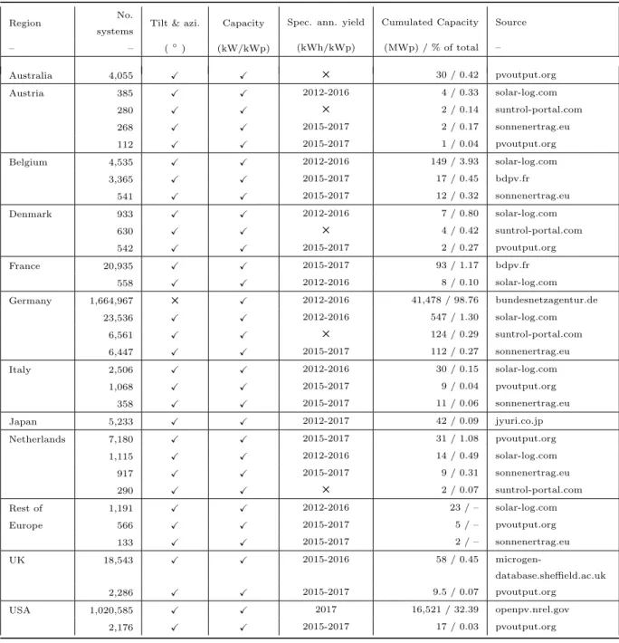
Table 1: Regions, parameters and data sources. “Rest of Europe” contains different European countries not already listed with less than 1,000 systems each. The cumulated capacity is given in MWp and, where available, as a relative share of the total installed capacity in a region (own calculations based onIEA(2018) with data from 2016 andNational Grid UK(2018) in case of UK with data from 2018).
Region No.
systems Tilt & azi. Capacity
Spec. ann. yield Cumulated Capacity Source
– – (◦) (kW/kWp) (kWh/kWp) (MWp) / % of total – Australia 4,055 X X 5 30 / 0.42 pvoutput.org Austria 385 X X 2012-2016 4 / 0.33 solar-log.com 280 X X 5 2 / 0.14 suntrol-portal.com 268 X X 2015-2017 2 / 0.17 sonnenertrag.eu 112 X X 2015-2017 1 / 0.04 pvoutput.org Belgium 4,535 X X 2012-2016 149 / 3.93 solar-log.com 3,365 X X 2015-2017 17 / 0.45 bdpv.fr 541 X X 2015-2017 12 / 0.32 sonnenertrag.eu Denmark 933 X X 2012-2016 7 / 0.80 solar-log.com 630 X X 5 4 / 0.42 suntrol-portal.com 542 X X 2015-2017 2 / 0.27 pvoutput.org France 20,935 X X 2015-2017 93 / 1.17 bdpv.fr 558 X X 2012-2016 8 / 0.10 solar-log.com Germany 1,664,967 5 X 2012-2016 41,478 / 98.76 bundesnetzagentur.de 23,536 X X 2012-2016 547 / 1.30 solar-log.com 6,561 X X 5 124 / 0.29 suntrol-portal.com 6,447 X X 2015-2017 112 / 0.27 sonnenertrag.eu Italy 2,506 X X 2012-2016 30 / 0.15 solar-log.com 1,068 X X 2015-2017 9 / 0.04 pvoutput.org 358 X X 2015-2017 11 / 0.06 sonnenertrag.eu Japan 5,233 X X 2012-2017 42 / 0.09 jyuri.co.jp Netherlands 7,180 X X 2015-2017 31 / 1.08 pvoutput.org 1,115 X X 2012-2016 14 / 0.49 solar-log.com 917 X X 2015-2017 9 / 0.31 sonnenertrag.eu 290 X X 5 2 / 0.07 suntrol-portal.com Rest of 1,191 X X 2012-2016 23 / – solar-log.com Europe 566 X X 2015-2017 5 / – pvoutput.org 133 X X 2015-2017 2 / – sonnenertrag.eu UK 18,543 X X 2015-2016 58 / 0.45 microgen-database.sheffield.ac.uk 2,286 X X 2015-2017 9.5 / 0.07 pvoutput.org USA 1,020,585 X X 2017 16,521 / 32.39 openpv.nrel.gov 2,176 X X 2015-2017 17 / 0.03 pvoutput.org
Longitude and latitude: In cases where this 340
information was not provided, the geographical co-341
ordinates were derived from OpenStreetMap using 342
other given information such as the zip-code, city 343
name, state name, etc. Erroneous locations outside 344
the specific region are set NA. For confidentiality 345
reasons geographic information was provided sep-346
arately from the other parameters in case of the 347
18,543 systems from Sheffield Solar. The derived 348
longitude and latitude are not required to be highly 349
accurate to suit the needs of this paper as they are 350
purely used for trend analysis when studying rough 351
relationships to other parameters and for visualiza-352
tion purposes. The ability to allocate a PV system 353
to a specific country is certain in all cases. 354
Tilt and azimuth: Unfortunately, this impor-355
tant metadata is not available from all sources. In 356
case of Australia the provided data was imprecise 357
(45◦ steps in the azimuth) and thus estimated by
358
the approach described in Killinger et al. (2017b)
359
and improved inKillinger et al.(2017a) as the PV
360
power data was available. As Australia is on the 361
southern hemisphere, azimuth angles were trans-362
formed to normalise the angles expressed for both 363
hemispheres. Within this paper, we consider −90◦
364
to be east, 90◦ to be west, with 0◦ representing
365
south in the Northern hemisphere and north in the 366
Southern hemisphere. Multi-array systems are not 367
considered in this paper. In a few of the listed
368
datasets, an excessive amount of tilt values with 369
0◦ or 1◦and azimuth values of −180◦ are reported.
370
E.g. the Australian dataset reported 36% of all sys-371
tems having a tilt angle ≤ 1◦. Visual inspections
372
based on aerial images and results from the afore-373
mentioned parametrisation, however, showed that 374
such small tilt angles were very rare and regularly 375
incorrectly reported. From previous work with var-376
ious datasets, we know that such boundary values 377
are sometimes used as a default when data is miss-378
ing. As we have no quality control measures on the 379
data, the validity of the data at these boundary val-380
ues is in question and so are removed from consid-381
eration. Tilt ≤ 1◦ or > 89◦ and azimuth < −179◦ 382
or > 179◦ are thus set NA.
383
Specific annual yield: There are many
in-384
stances of systems reporting a specific annual yield 385
of 0 kWh/kWp. Without further information
386
from the datasets, it is not possible to distinguish 387
whether this is a default value for missing data or a 388
valid measurement. We expect that both cases reg-389
ularly occur and so we must remove any input of 390
0 kWh/kWp from our analysis. Furthermore, the 391
specific yield of a system is set NA if it was installed 392
within the year of consideration to ensure that a full 393
year of generation is the basis for the annual yield. 394
In order to compensate annual meteorological fluc-395
tuations within a dataset of a country, all values 396
within a year are divided by the ratio between the 397
mean value from all systems in this year and the av-398
erage of the mean values from all reported years. A 399
similar approach is applied inLeloux et al.(2012a). 400
In datasets reporting a continuous time series, the 401
specific annual yield was derived by the summation 402
of the normalised PV power values. Only systems 403
which have less than 10 days / ≈ 2.7% of miss-404
ing time steps in their generation data are consid-405
ered. The vast minority of systems in the datasets 406
reported specific annual yield values that signifi-407
cantly exceed any meteorological potential. We be-408
lieve that such values are either erroneous reports 409
of either yield or the installed capacity, as the lat-410
ter is used in some datasets to derive the former 411
through division. Whereas Taylor (2015) applied
412
a statistical based upper limit for outliers, a fixed 413
limit of 2,000 kWh/kWp was used in this paper. 414
The fixed value was chosen to ensure a reliable fil-415
tering even though the quality and range of values 416
may differ for the various datasets. A threshold
417
value of 2,000 kWh/kWp acknowledges the increas-418
ing risk of erroneous data beyond this value and is 419
a very cautious limit with the aim of avoiding any 420
erroneous filtering. In fact, this limit was only ex-421
ceeded in 2.65% of all systems that reported a yield 422
value from openpv.nrel.gov where we observed the 423
largest values within the study and only for 0.084% 424
of all systems in this study. 425
Please note that, regarding the installed capac-426
ity, no pattern was recognised that led us to be-427
lieve that there were any systematic quality issues. 428
The same applies for the other parameters that were 429
only available for some datasets, such as informa-430
tion about the network connection for Germany as 431
visualised in Figure 2. Hence, the data was taken
432
on an as-is basis in these cases. 433
A summary of the impact of our proposed qual-434
ity control criteria is provided in the appendix in 435
Table A.5 where percentages of removed data are
436
presented. Data from pvoutput.org were strongly 437
affected by the filtering of the low tilt values and 438
justify the need of such a quality control. There 439
is a significantly higher share of systems filtered 440
by < −179◦ when compared to the filter for
az-441
imuths > 179◦. This is because south is defined
442
as 180◦ in some datasets and are therefore
trans-443
formed by subtracting 180◦. Invalid entries in the
444
same datasets were defined as 0◦ and subsequently
445
filtered post-transformation by the lower threshold 446
value for azimuth values. Insufficient information 447
was given to derive the exact location for PV sys-448
tems, mostly from pvoutput.org. All valid parame-449
ter entries that have passed the quality control are 450
used for the analysis in the next two sections. 451
3. Analysis of PV system metadata 452
3.1. Analysis of parameters and dependencies 453
The datasets presented in section 2are very
in-454
homogeneous with large differences in the number 455
of systems in each region and the availability of 456
parameters. Before starting to explore individual 457
clusters, typical ranges of these parameters and po-458
tential dependencies between them shall be studied 459
on a global dataset. The general principle of the 460
global dataset is that every region has the same 461
weight. Consider Table 1, should all data be used
462
to make global statistics, the results would be bi-463
ased towards the countries with more data (USA 464
and Germany). Therefore, a normalisation method 465
must be employed to weight countries equally. Its 466
derivation follows the following procedure: 467
(1) Specific annual yield is the only parameter 468
that exists multiple times for each PV system. To 469
evenly weight all systems, only one normalised spe-470
cific yield value per system is considered by ran-471
domly selecting a year. This procedure was pre-472
ferred to others such as e.g. taking the mean value 473
for all values of a system in order to conserve sys-474
tem specific variability between years. (2) For each 475
combination of two parameters (e.g. tilt and spe-476
cific annual yield) the algorithm counts the number 477
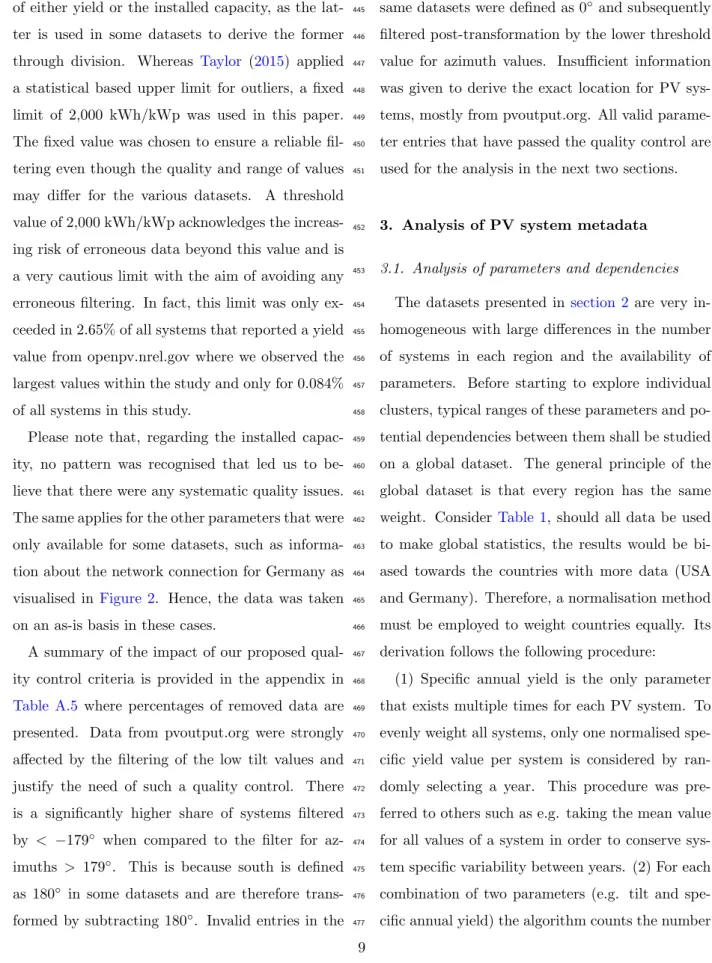
Figure 1: Hybrid graphic with plots of the different parameter pairs from the global dataset. The plots below the diagonal are scatter plots with the 25%, 50% and 75% quantiles as coloured lines. Plots on the diagonal are 1D-histograms of that parameter. Plots above the diagonal are 2D-histograms of the parameter pairs; the change in colour from white to red is an indication of probability and its distribution. The 2D-histograms and scatter plots have the parameter of their column on the x-axis and the parameter of their row on the y-axis. Note that each scatter and 2D-histogram pair have opposite axes but are identical data. 1D-histograms are the only exception with having displayed the density on the y-axis. For reasons of simplification the absolute value of the latitude is taken in these plots to make results from the northern and southern hemisphere comparable. The bold number in each plot shows the number of countries (n) which are considered in the plot as well as the sampling size (si).
of couples per region that have valid reports in both 478
parameters that have passed the quality control in 479
section 2. Only regions with a sample size of at
480
least 500 complete couples are considered to ensure 481
statistical relevance. (3) The smallest number of 482
complete couples from all regions is taken to de-483
fine the sample size for the global dataset. This 484
way, the same number of complete couples is taken 485
from each region. Therefore, all of the data is con-486
sidered for the region with the smallest number of 487
complete couples. In all other regions, the same 488
number of couples is randomly selected. To avoid 489
under-representation of larger systems, the selec-490
tion probability is linearly weighted with installed 491
capacity, not frequency. 492
The significant advantage of this procedure is 493
that regional characteristics are evenly weighted 494
and the availability for each pair of parameters is 495
individually considered. The disadvantage is that 496
many systems are randomly banned due to the re-497
gion with least availability. We applied different 498
methods of sub-sampling the data, however, the re-499
sulting global data was quite insensitive to differ-500
ent sampling procedures indicating the robustness 501
of our approach. 502
Results from the global dataset are displayed 503
in Figure 1 and the following observations can be
504
made: 505
Latitude: To have a robust quantity of data, 506
PV systems in latitudes between 30◦ and 55◦ are
507
studied. Latitude does not show any obvious in-508
fluence to the installed capacity or azimuth angle. 509
The tilt angle shows a tendency to increase with 510
an increasing latitude, corroborating the same ob-511
servation byPfenninger and Staffell(2016) between
512
the latitude ranges in the study. This finding agrees 513
with studies showing that systems should have a 514
smaller tilt closer to the equator in order to opti-515
mise their annual yield (S´ˇuri et al.,2007). It is still 516
surprising since many systems in our analysis are 517
installed on roofs and strongly depend on the roofs’ 518
inclination. It can be suggested that the roof pitch 519
has a tendency to be steeper at higher latitudes in 520
our datasets and agrees with similar observations in 521
Europe (McNeil,1990, p. 883). Furthermore, a
lin-522
ear decline in the specific annual yield is observed 523
with an increasing latitude. This occurs in accor-524
dance to the tendency of a higher solar potential in 525
regions closer to the equator (ˇS´uri et al.,2007). 526
Installed capacity: Within the plot, only sys-527
tems < 100 kWp are displayed for ease of visuali-528
sation. Even though the sampling weights in pref-529
erence of larger systems, there is a clear concentra-530
tion of smaller system sizes. There is a visual trend 531
towards smaller tilts with an increasing installed 532
capacity. Furthermore, there is a clear observation 533
that larger capacity systems are consistently ori-534
ented towards the equator whereas smaller systems 535
have a much broader range of orientation. A depen-536
dency between the installed capacity and the spe-537
cific annual yield cannot be observed in the global 538
dataset. Despite that, we would expect that the 539
efficiency of larger systems is usually higher and 540
systems better maintained. Most likely, this trend 541
is invisible here since data from many geographic 542
regions were sampled. This hypothesis is checked 543
in section 4. The finding that PV system size has
544
interdependencies on the other parameters can be 545
reaffirmed with everyday observations; smaller sys-546
tems are in most cases mounted on the roof of res-547
idential buildings, medium systems are typically 548
found on farming houses or industrial buildings, 549
and large systems are mounted on a rack on the 550
ground. 551
Tilt: Tilt in the dataset mainly occurs in a range 552
up to 50◦ and is often reported in steps of 5◦,
553
though reporting steps of 10◦are also common. No
554
discernible trend between tilt and azimuth is ob-555
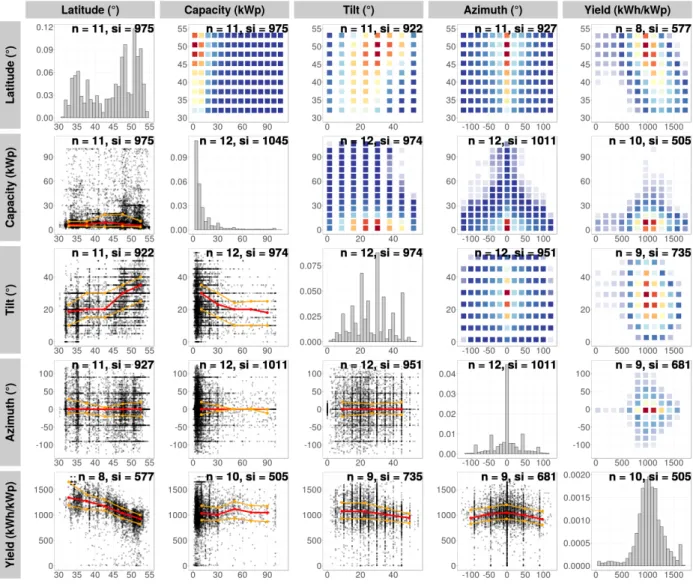
Figure 2: The installed capacity and its relationship to the relative share of systems for different countries (left). The line width and colours vary to simplify the differentiation. The cumulative installed capacity in case of Germany is shown in the right plot represented by the coloured line (colouration indicating the network connection) whereas the black line represents the cumulative number of systems. The dashed line indicates 25 kWp, which is used to sub-categorise the data insection 3.2.
served, however the 2D-histogram shows a signifi-556
cant density peak around the most frequent combi-557
nation of azimuth and tilt with a radially decreasing 558
probability, this was also observed bySaint-Drenan
559
(2015); Killinger et al. (2017c). A decrease in the
560
specific annual yield can be seen with an increas-561
ing tilt. This might be caused by the finding that 562
tilt is usually smaller for decreasing latitudes which 563
occur in combination with an increased specific an-564
nual yield. 565
Azimuth: There is a significant peak of azimuth 566
angles pointing south (north in Australia). It is
567
probable that this distinct peak is due to the tar-568
geted approach of solar installers who favour equa-569
torial orientated rooftops due to performance ben-570
efits. Indeed, azimuth angles tend towards reach-571
ing a higher specific annual yield with systems ori-572
ented towards 0◦. In general, outliers reach a range 573
of +/- 100◦ with discrete reporting intervals being
574
visible in the 1D-histogram and scatter plot, e.g. 575
databases only requiring azimuth reported to near-576
est 15◦. 577
Specific annual yield: The 1D-histogram of 578
yield shows the most distinct shape of all param-579
eters with a peak around 1,000 kWh/kWp. Fur-580
thermore, there is a small peak at 1,650 kWh/kWp 581
which is caused by PV systems in southern re-582
gions of the USA. It is not possible with the lim-583
ited latitude study area to infer that the regression 584
of specific yield with latitude will extend towards 585
the equator; climatic regions are expected to be 586
far more influential on the specific yield whereby 587
around the equator there is a significant presence 588
of clouds, and around the tropics there tends to be 589
desert. It is probable that the secondary peak above 590
1,650 kWh/kWp is for systems installed in particu-591
larly arid regions found in southern USA, however, 592
climatic influence is outside the scope of this paper 593
and is reserved for future study. The specific an-594
nual yield has the most visually recognisable trends 595
to all other parameters, demonstrating the strong 596
inter-relationship. There is a need for a more de-597
tailed multi-variable analysis between specific an-598
nual yield and the other parameters. However, due 599
to its extra complexity it falls outside the scope of 600
this paper. 601
3.2. Representativeness of clusters 602
In the previous section, important characteris-603
tics of PV systems and their dependencies were de-604
rived. With exception of the annual specific yield 605
and installed capacity in Germany, metadata of all 606
the installed systems within the different regions 607
is not known (e.g. we have access to 4,055 systems 608
from Australia when there are an estimated 1.8 mil-609
lion installed). This restriction questions the rep-610
resentativeness and re-usability of our observations 611
when using the statistics of a subset of systems to 612
infer the statistics of the remainder because some 613
characteristics could be over- or underrated in our 614
datasets. To achieve representation, a solution is to 615
sub-categorise metadata from the PV systems into 616
smaller and more homogeneous clusters. By doing 617
so, an end-user can use the statistics of the clusters 618
and weight them individually by the probability of 619
occurrence. Prior to an approximation of metadata 620
insection 4, it is the objective within this section to
621
define groupings or clusters of PV system that allow 622
the derivation of representative characteristics. 623
The interdependency analysis reveals two domi-624
nating parameters which show multiple dependen-625
cies to others: (1) The installed capacity and (2) 626
a geographical influence (c.f. absolute latitudes
627
are used to account for hemispheres). These two 628
findings are in accordance with K¨uhnert (2016);
629
Saint-Drenan (2015); Saint-Drenan et al. (2017)
630
who analysed azimuth and tilt for different classes 631
of installed capacity and multiple regions. Such
632
a separation has the benefit to acknowledge the 633
impact from these two dominating parameters on 634
others, while still allowing us to derive meaning-635
ful statistics within a chosen cluster. As K¨uhnert
636
(2016) evaluates, a balance must be found between
637
the number and size of the clusters, in order to guar-638
antee that each class includes a sufficient number of 639
data to be representative. 640
The left plot inFigure 2provides further insights 641
into the system size and its relative share for differ-642
ent countries in this paper. Differences can be ob-643
served between countries but all show a heightened 644
concentration towards small scale systems with a 645
relative share between 60% (Germany) and 99% 646
(UK) of systems < 10 kWp. Whereas most datasets 647
only cover a selection of systems within a country, 648
the dataset in case of Germany (bundesnetzagen-649
tur.de) covers the vast majority of systems and is 650
detailed on the right plot. Almost one million out 651
of the 1.6 millions German systems are smaller than 652
10 kWp but in total, with an aggregated capacity 653
of ≈ 5 GWp, they only represent ≈ 12% of the 654
installed capacity. Another 650,000 systems occur 655
in a range between 10 and 100 kWp and cover ad-656
ditional ≈17.5 GWp. Only 35,000 systems are > 657
100 kWp yet are responsible for half of the total 658
installed capacity. 659
On the search of a threshold value to split the 660
datasets into representative clusters, a system size 661
of 25 kWp was chosen by considering: (1) An in-662
stalled capacity of 25 kWp is an adequate size 663
between typical roof mounted systems and larger 664
plants, particularly as larger capacities are linked 665
to larger physical space requirements. (2) So even 666
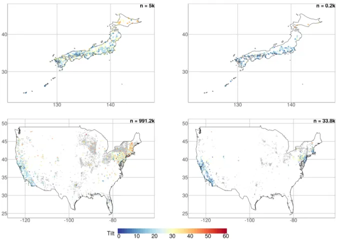
Figure 3: Maps for Australia (top) and Europe (bottom). The left column shows systems ≤ 25 kWp and the right column systems > 25 kWp. Systems which do not report tilt are in grey colour.
though the number of larger systems is rather low in 667
most countries, their strong contribution to the to-668
tal power generation and the knowledge that char-669
acteristics change with the system size justify a con-670
sideration in a separate cluster. The threshold value 671
of 25 kWp is displayed as a dashed vertical line in 672
Figure 2. If the threshold value were higher, only a
673
small number of systems would be left in the upper 674
cluster and the derivation of representative statis-675
tics impeded. (3) Several threshold values were tri-676
alled in our analysis. A value of 25 kWp was finally 677
decided upon as it satisfied the aforementioned cri-678
teria and passed visual inspection by producing dis-679
tinct distribution curves. 680
Both the impact of system size and the geograph-681
ical influence can be studied in respect to the tilt 682
angle of systems in Figure 3and Figure 4. All
re-683
gions show a tendency towards smaller tilt angles 684
for system sizes > 25 kWp. Especially for systems 685
≤ 25 kWp in Europe, the dependency between lat-686
itude and tilt can be observed by an increasing tilt 687
angle from Italy to Denmark. However, it should 688
be noted that the spatial influence is not only lim-689
ited to a pure geographical relationship; the spatial 690
impact depends on regulations and incentives which 691
often occur on a national level. The policy situation 692
Figure 4: Maps for Japan (top) and the USA (bottom). The left column shows systems ≤ 25 kWp and the right column systems > 25 kWp. Systems which do not report tilt are in grey colour.
in France leads to a high number of 3 kWp systems 693
(see Leloux et al.(2012b) in section 1.1). In
Ger-694
many, there are changing regulations and feed-in 695
tariffs for systems > 30 kWp resulting in an in-696
crease in the black line of the right plot inFigure 2. 697
Furthermore, the UK had a higher feed-in tariff for 698
systems ≤ 4 kWp up until January 2016 and has 699
since moved to ≤ 10 kWp (ofgem,2018). These are
700
such examples of significant policy-specific regional 701
influence that can impact upon the characteristics 702
of PV systems. 703
There are many opportunities as to how we sub-704
categorise the data into clusters. Many of which 705
could be explored in order to derive meaningful 706
information depending on the approach. Options 707
include separating by climatic region or grouping 708
by policy similarities. However with respect to the 709
aforementioned aspects, a clustering at a country 710
level seems advisable for the following reasons: (1) 711
National regulations and incentives have a visually 712
evident impact on the occurrence of different sys-713
tem sizes which may itself influence other metadata. 714
(2) A geographical influence was observed on mul-715
tiple parameters. Countries limit this influence by 716
their size. The only exception of this strategy is the 717
USA. The enormous geographic area of this country 718
results in a inhomogeneous pattern of the specific 719
annual yield. This is a direct consequence of the 720
heterogeneity of the solar resource within a country. 721
The USA was thus split at 37.5◦ N into a northern
722
and a southern component. The same approach
723
could be applied to Australia, however, the sample 724
size of available data is too low. Further subdivi-725
sions e.g. by the latitude for systems ≤ 25 kWp in 726
France (see tilt in Figure 4), could be considered
727
but exceed the scope of this paper and is a focus 728
of future work. (3) There is a certain convenience 729
to clustering by countries. Many of the studies pre-730
vious focused mainly on a single country, this is 731
indicative of a researchers interests and data avail-732
ability. We feel that, whilst there are many options 733
of clustering that can be explored, a preliminary 734
study at a country level is of most interest. 735
The region ``Rest of Europe” is not be consid-736
ered further due to its inhomogeneous portfolio of 737
systems across different countries in Europe. The 738
clusters, defined by their belonging to a region and 739
system size, are used in the next section to derive 740
representative distributions for the metadata. 741
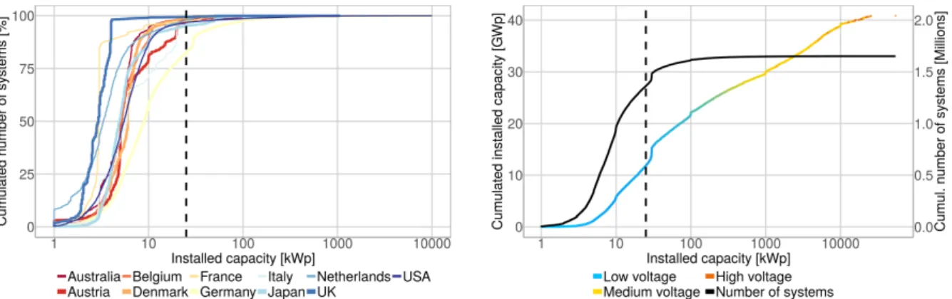
Australia Logistic RMSE = 2% n = 1.1k = 0.86 50 Prob. Dens. (%) 0 -180 0 180 Austria Logistic RMSE = 6% n = 985 = 0.79 -180 0 180 Belgium Logistic RMSE = 3.4% n = 8.2k = 0.83 -180 0 180 Denmark Logistic RMSE = 7.3% n = 2k = 0.66 60 -180 0 180 France tLoc.Scale RMSE = 3.4% n = 20.5k = 0.85 -180 0 180 Germany Logistic RMSE = 5% n = 29.6k = 0.76 -180 0 180 Italy tLoc.Scale RMSE = 5.4% n = 3.6k = 0.67 -180 0 180 Japan Logistic RMSE = 9.6% n = 5k = 0.65 70 -180 0 180 Netherlands Stable RMSE = 5.8% n = 8.6k = 0.81 -180 0 180 UK Logistic RMSE = 2.1% n = 20.4k = 0.91 -180 0 180 USA North Logistic RMSE = 2.6% n = 171.9k = 0.86 -180 0 180 USA South Logistic RMSE = 5.6% n = 165.3k = 0.62 -180 0 180 Azimuth (°) Logistic RMSE = 1.2% n = 1.1k = 0.99 50 Prob. Dens. (%) 0 0 45 90 Weibull RMSE = 2.5% n = 946 = 0.95 0 45 90 Extr.Val RMSE = 3.3% n = 8.2k = 0.93 0 45 90 Loglogistic RMSE = 4.7% n = 2k = 0.82 0 45 90 Lognormal RMSE = 4.1% n = 20.6k = 0.84 0 45 90 Extr.Val RMSE = 2% n = 29.6k = 0.96 0 45 90 Stable RMSE = 2.3% n = 3.3k = 0.96 0 45 90 Extr.Val RMSE = 13.5% n = 5k = 0.6 0 45 90 Extr.Val RMSE = 3% n = 7.4k = 0.88 0 45 90 tLoc.Scale RMSE = 3% n = 19.8k = 0.97 0 45 90 Loglogistic RMSE = 2% n = 174.3k = 0.97 0 45 90 tLoc.Scale RMSE = 0.7% n = 181.4k = 1 0 45 90 Tilt (°) tLoc.Scale RMSE = 2% n = 4k = 0.96 50 Prob. Dens. (%) 0 0 12 25 Gen.Extr.Val RMSE = 6% n = 1k = 0.64 0 12 25 Stable RMSE = 1.1% n = 8.3k = 0.98 0 12 25 tLoc.Scale RMSE = 2.6% n = 2.1k = 0.93 0 12 25 Stable RMSE = 5% n = 20.6k = 0.99 100 0 12 25 Gen.Extr.Val RMSE = 0.8% n = 1404.1k = 0.97 0 12 25 Stable RMSE = 3.8% n = 3.8k = 0.8 0 12 25 Stable RMSE = 1% n = 5k = 0.99 0 12 25 tLoc.Scale RMSE = 0.8% n = 9.3k = 1 0 12 25 Stable RMSE = 1.7% n = 20.7k = 0.99 0 12 25 Gen.Extr.Val RMSE = 0.5% n = 393.1k = 1 0 12 25 Burr RMSE = 0.3% n = 542k = 1 0 12 25 Capacity (kWp) No Data 50 Prob. Dens. (%) 0 0 1 2k tLoc.Scale RMSE = 0.7% n = 1k = 1043 0 1 2k Burr RMSE = 1.4% n = 15k = 922 0 1 2k Stable RMSE = 1.4% n = 2.1k = 784 0 1 2k tLoc.Scale RMSE = 0.3% n = 23.3k = 1101 0 1 2k Stable RMSE = 0.9% n = 5885k = 862 0 1 2k tLoc.Scale RMSE = 0.6% n = 5.4k = 1143 0 1 2k Burr RMSE = 0.5% n = 10.8k = 1221 0 1 2k Stable RMSE = 0.6% n = 6.2k = 853 0 1 2k Stable RMSE = 1.3% n = 28.7k = 897 0 1 2k Stable RMSE = 1.9% n = 111.9k = 1014 0 1 2k Extr.Val RMSE = 4.6% n = 73.1k = 1432 90 0 1 2k Yield (kWh/kWp) Figure 5: Histograms of real data (bar) with appro ximated probabilit y distributions (line) for the differen t clusters (columns) and parameters (ro ws), where capacit y is the installed capacit y and yield is the sp ecific ann ual yield. All systems rep orted within this figure ha v e a capacit y ≤ 25 kWp, see a pp endix for the same plot for > 25 kWp. Within ea ch of the a xes is rep orted the name of the b est fitting distribution typ e (see section 4.1 for detail), the ro ot mean squared error (RMSE) b et w een the scatter of real data in the histogram against the fitted probabilit y densit y dis tr ibu ti o n, the n um b er of data p oin ts con si dered for that cluster (n ), and the P earson correlation co effici en t (ρ ) of the linear regression. The mean v alue µ is sho w n in pl a ce o f ρ for Yield. All y-axes a re sc a led b et w een 0% and 50% probabilit y except where a b old red v alue is assigned to the individual axis.
4. Approximation of parameters in clusters 742
The intentions of parametrisation are twofold. 743
Firstly, we want to discover whether or not the pa-744
rameters (tilt, azimuth, capacity and yield) can be 745
represented with simple parametric distributions. 746
Secondly, we want to explore the relative differ-747
ences between clusters through comparison between 748
probability distributions. We concede that simple 749
distribution fitting has weaknesses such as not ap-750
propriately capturing a more complex relationship 751
offered by non-parametric fitting, however, repro-752
ducibility of the statistics is encumbered with added 753
complexity. For our first presentation of the sub-754
stantial volume of PV system data collected, we 755
focus on simple distribution fitting as interesting 756
comparisons and individual cluster insights can be 757
drawn, and we are able to comment on the ability 758
for these complex parameters to be represented as 759
such. 760
4.1. Methodology of fitting the distributions 761
In order to enable the utilisation of the aggre-762
gated statistics of each cluster (defined in
sec-763
tion 3.2) and for each parameter (defined in
sec-764
tion 3.1), individual distributions are fitted to the
765
real-world probability density histograms. The re-766
sults are presented inFigure 5(≤ 25 kWp) and
Fig-767
ure A.10(> 25 kWp). The total number of
avail-768
able data varies between clusters and parameters; 769
there is no further processing beyond the criteria 770
described in section 2; all possible data available
771
is used. Differences in data within a cluster are
772
due to some PV sites not reporting one or more 773
parameters. There are up to 6 years of reported 774
specific annual yield (2012-2017). The normalised 775
value within each year is taken as an individual 776
sample and so there are up to 6n more samples for 777
this parameter. 778
For each cluster and for each parameter, many 779
different distribution types were fitted to the 780
probability density. Distributions were fit
us-781
ing the inbuilt fitdist function of the software 782
Matlab (R Matlab,2018). There are 23 parametric
783
distribution types available, of which all are fitted 784
to the data. Where distribution types require only 785
positive values (for parameters with negative bins) 786
or values between 0 and 1, the data is scaled to sat-787
isfy the distribution requirements and allowed to re-788
scale so that as many distributions could be tested; 789
note that no distribution requiring this treatment 790
was found to be best fitting, and so no further 791
discussion is made regarding this normalising pro-792
cess. Probability density functions are then scaled 793
to only exist between the x-axes limits as indicated 794
in the figure, for example, the tilt distributions are 795
only relevant between 0◦ and 90◦. This means that
796
the sum of all probabilities between the prescribed 797
x-axis range must be equal to 1. This is important 798
as some distributions facilitate values way outside 799
of the bin limits resulting in the sum of probabili-800
ties between the bins of interest 6= 1, and so would 801
not fit the histogram. The disclaimer is, therefore, 802
that these distributions must be scaled before use 803
and not be extrapolated beyond the specified bin 804
ranges else risk persisting an under/overestimation 805
about the scaling factor, defined as 806
s = 1
Pb
apa:b
where s is the scaling factor, p is the probability 807
at each bin between the lower and upper bin limit, 808
a and b, respectively. The resultant fitted distribu-809
tion is then plotted against the real probability den-810
sity and tested for linear fit; the root mean squared 811
error (RMSE, percentage) and Pearson correlation 812
coefficient (ρ, dimensionless) are derived. A per-813
fectly fitted distribution would result in y = x with 814
ρ = 1 and an RMSE= 0%. The distribution type 815
with the lowest RMSE was selected for the plot. 816
Should there be more than one distribution type 817
that has the same RMSE, then the type with low-818
est ρ is selected. Should there still be more than 819
one distribution type after this, one of the remain-820
ing types is selected at random. 821
The exact parameterisation for each distribution 822
presented inFigure 5andFigure A.10are detailed
823
in Table A.4. Each distribution has up to 4
co-824
efficients and are employed using different equa-825
tions, not all 23 parametric distributions are de-826
tailed, only those that featured within the study. 827
Whilst Table A.4 details the parameterisation of
828
the coefficients, it is Table A.3 that explains how
829
to use those values to form the distribution. Fur-830
thermore, the mean or median values of the whole 831
dataset, exclusive of the 25 kWp separation, are 832
presented inTable 2.
833
4.2. Discussion of the distributions 834
The following discussion about clusters and dis-835
tributions mainly refers to Figure 5 with systems
836
≤ 25 kWp unless explicitly noted otherwise. The 837
reason for this is that the vast majority of systems 838
are within the ≤ 25 kWp category, and so are of 839
most interest. However, important differences to 840
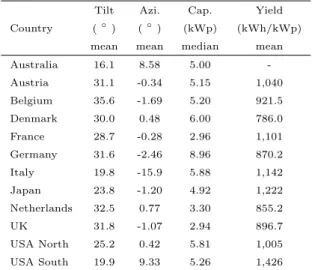
Table 2: Mean or median value extracted from entire data set (without separation by capacity size) for each of the pa-rameters of tilt angle, azimuth angle, system capacity and specific annual yield.
Tilt Azi. Cap. Yield
Country (◦) (◦) (kWp) (kWh/kWp)
mean mean median mean
Australia 16.1 8.58 5.00 -Austria 31.1 -0.34 5.15 1,040 Belgium 35.6 -1.69 5.20 921.5 Denmark 30.0 0.48 6.00 786.0 France 28.7 -0.28 2.96 1,101 Germany 31.6 -2.46 8.96 870.2 Italy 19.8 -15.9 5.88 1,142 Japan 23.8 -1.20 4.92 1,222 Netherlands 32.5 0.77 3.30 855.2 UK 31.8 -1.07 2.94 896.7 USA North 25.2 0.42 5.81 1,005 USA South 19.9 9.33 5.26 1,426
system sizes > 25 kWp are mentioned and can be 841
observed inFigure A.10.
842
It is important to note that only rough dependen-843
cies between parameters, regions and system sized 844
can be considered with this clustering approach. 845
The more intricate and established interdependen-846
cies have not been explored within this paper as it 847
is beyond the scope of the initial objective. The 848
authors reserve this for future work. 849
4.2.1. Azimuth angle 850
The most noticeable feature of the azimuth ob-851
servations is the significant probability of an equa-852
torial facing PV system. This is unsurprising as 853
it offers the best annual specific yield by receiving 854
maximum system efficiency at peak solar position. 855
The topic of extreme probability of an equatorial 856
orientated system was discussed in section 3.1; the
857
prevalence of 0◦is true of all sites for both < 25 and 858
> 25 kWp. The Japan and Netherlands clusters 859
have exaggerated angles of -45◦ or +45◦, assumed 860
to be a result of overly simplified reporting. 861
The distributions could not capture the probabil-862
ity of 0◦ with exception of the Netherlands where
863
a Stable distribution fitted best. Even with large 864
sample sizes for the USA North and south clusters, 865
a distribution could not be fitted that satisfied the 866
observed probability for an azimuth angle of 0◦.
867
Perhaps a more complex or bespoke distribution 868
type is needed to suitably express the probability 869
distribution of azimuth angle with reproducible ac-870
curacy. This large proportionality of 0◦ was also
871
observed bySaint-Drenan et al.(2018), who fitted
872
a normal distribution in similar magnitudes to the 873
logistical distribution fitted in this article. That 874
said, there is an argument that the significant 0◦ az-875
imuth feature is exaggerated when considering the 876
UK cluster. The majority of the data within the UK 877
cluster is from Sheffield Solar. Their users report 878
the system metadata, however, there is a feedback 879
to the user reporting system performance analysis 880
on a monthly basis, inclusive of a nearest-neighbour 881
performance analysis of a system of similar meta-882
data. Users are encouraged to verify their reported 883
metadata and is often double checked with satellite 884
imagery; the result is much more accurate report-885
ing of metadata for the UK cluster leading to the 886
smoothness of distribution fit. With improved PV 887
system metadata reporting, we see a wider spread 888
of azimuth about 0◦. 889
4.2.2. Tilt angle 890
The tilt angle across all clusters is rather unique 891
per cluster with 7 different distribution types be-892
ing found as the best fitting among 10 clusters. We 893
previously discussed the gentle increase of tilt an-894
gle with latitude. Solar installers can mount the PV 895
panels with a steeper tilt angle to that of the roof at 896
higher latitudes through arrangement of the mount-897
ing brackets; this is not expected to be overly com-898
mon practise. The predominant factor for smaller 899
roof integrated systems is expected to be the phys-900
ical roof angle, which is influenced by local archi-901
tectural styles. We suspect this is the case, partic-902
ularly when considering France in Figure 3 where
903
there exists a distinct change in the tilt for the ≤ 25 904
kWp systems at roughly 47.5◦ latitude. Note that
905
France and Denmark have similar distributions de-906
spite France having a significant number of systems 907
south of that 47.5◦ roof tilt feature. Furthermore,
908
Belgium and the Netherlands share similar climate 909
and latitude yet feature distinctive distributions. 910
Interestingly, the Australian cluster consisting of 911
the second lowest number of observations has the 912
second most accurate fit after USA South. This 913
is in part due to the smoothness of the distribu-914
tions and accuracy of method in which the tilt is 915
obtained (seesection 2). The USA cluster has
excel-916
lently fitted distributions suggesting accurate mea-917
surement, particularly for the USA South cluster 918
where the tilt distribution is fitted with ρ = 1 and 919
RMSE=0.7%. The Japan cluster evidently suffers 920
from reporting to the nearest 10◦, and so we suggest 921
to avoid using a best-guess approach to collecting 922
metadata as it leads to biased distributions. The 923
tendency for larger system sizes having smaller tilt 924
angles, introduced in section 3.1, can be confirmed
925
when comparing Figure 5 and Figure A.10. The
926
only exception is Denmark, which reports only a 927
small number of systems > 25 kWp. 928
Within the distributions, the smallest mean tilt 929
angles were reported in Australia (16.07◦), Italy
930
(19.81◦) and USA South (19.89◦). The largest
931
mean tilt values were reported in Belgium (35.58◦)
932
and closely followed by the UK, Germany and Aus-933
tria (31◦). 934
4.2.3. Installed capacity 935
The most obvious observation from the installed 936
capacity is the extreme peak within the French clus-937
ter. Of all 20.6k systems (≤ 25 kWp and > 25 938
kWp), 73.74% of them report an installed capacity 939
of 3 kWp when rounded to nearest integer, though 940
note that the French dataset reported to a high dec-941
imal precision. The best fitting distribution cannot 942
appropriately represent this extreme despite a very 943
high ρ = 0.99; the RMSE value of 5% is indicative 944
of the Stable distribution assigning 100% probabil-945
ity to 3 kWp. This distribution is, therefore, very 946
limited even if it does most accurately capture the 947
data for France. As discussed when defining the 948
clusters, this peak in capacity is a direct response 949
to regulations within that country. This is further 950
observed in the UK database, with the vast major-951
ity of systems being ≤ 5 kWp due to the nature of 952
the feed-in tariff rate. The north and south USA 953
clusters demonstrate the power of a larger and con-954
sistent sample size reporting RMSE 0.5% and 0.3%, 955
respectively, with both reporting ρ = 1. Interest-956
ingly, the distribution type between USA clusters 957
are distinct from each other, with a slightly in-958
creased probability of smaller systems in the south. 959
This is expected to be a result of more rooftop solar 960
in the sunnier States, though this is speculation. 961
The shape of the distribution functions for sys-962
tem sizes > 25 kWp (Figure A.10) differ to systems 963
≤ 25 kWp and show an heightened concentration of 964
systems < 50 kWp. Australia is an exception and 965
reports many systems with an installed capacity of 966
≈ 100 kWp. 967
The mean values of capacity are too heavily in-968
fluenced by the presence of large systems (cf. 2b),
969
and so the median value is reported to reduce bias. 970
From the distributions, the country with smallest 971
capacity median is the UK (2.94 kWp) and the 972
largest is Germany (8.96 kWp). The fact that
973
the German data reveals such a high median is re-974
flective of the thorough nature of data collection 975
whereby nearly all systems are reported; we have 976
very few large systems reported from the UK as 977
the database is primarily used for rooftop solar and 978
so this statistic is not overly representative. 979
4.2.4. Specific annual yield 980
The most noticeable detail of the specific annual 981
yield distribution fits is the smoothness of the his-982
tograms of raw data. This is perceived to be of 983
two reasons. Firstly, the sample size is typically 984
much larger (n = 5.885m for the German clus-985
ter). Secondly, the data is digitally recorded and 986
not reliant on human reporting. The mean µ is
987
presented in place of the correlation coefficient so 988
as not to over busy the plot, though for complete-989
ness, all sites reported ρ ≥ 0.98 except USA South 990
with ρ = 0.93. Recall that the specific annual yield 991
is normalised for inter-annual differences and so we 992
can directly compare clusters. Each cluster exhibits 993
reasonably unique subtle traits, it is expected that 994
the larger the share of equatorial orientated systems 995
with more optimal tilts, the larger the specific yield, 996