Finite pure bending of curved pipes

HAL Id: hal-00111513

https://hal.archives-ouvertes.fr/hal-00111513

Submitted on 26 Sep 2019

HAL is a multi-disciplinary open access

archive for the deposit and dissemination of

sci-entific research documents, whether they are

pub-lished or not. The documents may come from

teaching and research institutions in France or

abroad, or from public or private research centers.

L’archive ouverte pluridisciplinaire HAL, est

destinée au dépôt et à la diffusion de documents

scientifiques de niveau recherche, publiés ou non,

émanant des établissements d’enseignement et de

recherche français ou étrangers, des laboratoires

publics ou privés.

Finite pure bending of curved pipes

D. Boussaa, K. Dang Van, P. Labbé, H. T. Tang

To cite this version:

D. Boussaa, K. Dang Van, P. Labbé, H. T. Tang. Finite pure bending of curved pipes. Computers

and Structures, Elsevier, 1996, 60 (6), pp.1003-1012. �10.1016/0045-7949(96)00011-9�. �hal-00111513�

FINITE PURE BENDING OF CURVED PIPES

Dj. Boussaa,t,t K. Dang Van,t P. Labbe§ and H. T. Tang�

tLaboratoire de Mecanique et d'Acoustique, CNRS, _31, chemin Joseph Aigmer, 13402 Marseille cedex 20, France

§Service Etudes et Projets Thermiques et Nucleaires, Electricite de France, Villeurbanne, France �Nuclear Power Division, Electric Power Research Institute, Palo Alto, CA, U.S.A

Abs

�

act-We present �n �riginal treatment for the finite bending of curved pipes with arbitrary cross sectiOns. The curved pipe IS successively regarded as a three-dimensional continuum and a shell and a

formulati�m is proposed for eac

?

model. We show that, from a numerical point of view, the finite

b

ending problem IS reductble to an axisymmetric analysis augmented with I d.f. We also show how to take

advantage of this analogy to solve the bending problem using standard axisymmetric FE routines.

l. INTRODUCTION

Curved pipes are among the most vulnerable com­ ponents of piping systems. When compared to straight pipes of the same cross section and length, real-life curved pipes prove much more flexible and suffer much more severe stresses under the same bending moment. This contrast is due to the ovaling of the curved pipe cross section during bending, a phenomenon that thus cannot be accounted for by the usual beam theory_

Even though the experimental discovery of the high flexibility of curved pipes is generally credited to Bantlin ( 1910), the above basic facts were actually known by the end of the 19th century. Piping systems of steamers were designed using beam theory, the extra flexibility of the curved parts being acounted for by multiplying their beam-stiffness by an empirical coefficient of 6/ 10, well-suited to the curved pipe geometries used at that time in naval engineering

[I].

As regards modeling, the earliest conclusive contribution, in the small displacement setting, is due to von Karman (191 1 ). Many attempts however preceded this work. In 190 I, as is reported in its

Comptes Rendus de l'Academie des Sciences

(pp. l057-1058), the French Academy of Sciences acknowledged the contribution of naval engineer Marbec to justify the flexibility coefficient of 6/ 10. Always in the small displacement setting, Clark

et al. [2, 3]

proposed general formulae which are commonly used in the design of piping systems. An illustration is provided by the rigidity factor l'f. Let 1/EI denote the beam flexibility of the curved pipe and lll'fEI its effective flexibility, respectively. Clark

t To whom correspondence should be addressed.

and Reissner

[2]

showed that IJ, for a wide range of geometries, is given by

(I) where fJt is the radius of curvature of the curved pipe, b the radius of its cross section assumed to be circular h its thickness assumed to be constant and v it

�

Poisson's ratio.

In the large displacement setting, many researchers have paid attention to the problem ((4-7] and refer­ ences therein). Except for the last reference, the treatment is purely analytical, involves many assump­ tions, and is based on Fourier series expansions which impose serious limitations (e.g. perfect ge­ ometries required) and suggests that more flexible solution techniques, such as the FE method, could prove better suited_

Guidelines are given in Ref. (8] to treat the curva­ ture controlled case using a standard axisymmetric FE analysis. A full formulation restricted to the small displacements case is developed in Ref. (9]. Moreover, it is shown in this reference that the FE dicretized pure bending problem may be regarded as an axisym­ metric analysis augmented with I d.f. In some re­ spects, our work may be inscribed as an extension of these two references, although we followed a different approach from those developed therein.

The paper is organized as follows. The second section is devoted to the statment of the problem in the full three-dimensional framework. The simi­ larities between this problem and an axisymmetric analysis are emphasized by a systematic decompo­ sition of the kinematics of the bending problem into an axisymmetric part and additional terms. In the

third section we reduce this three-dimensional formu­ lation to a shell formulation. In the fourth section, by resorting to a FE discretization, we derive a matrix statement of the problem. The similarities between the present problem and an axisymmetric analysis are accounted for and the discretized formulation is shown to be reducible to an axisymmetric problem augmented with I d.f. Finally, we present some numerical comparisons with existing results, followed by a brief conclusion.

2. THE CURVED PIPE AS A THREE-DIMENSIONAL CONTINUUM

2.1.

Notations

Throughout the paper, the symbol ® will denote the standard tensor product of two vectors ((x, y)�--+x®y) or two second order tensors ((X, Y)�--+X®Y), the dot the Euclidean inner product of two vectors ((x, y)�--+x, · y) or two second order

tensors ((X, Y)t--+X

·

Y = trace(XYT)).

2.2.

Kinematics

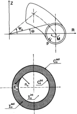
In its initial configuration assumed stress free, the curved pipe under study, shown in Fig. I with the main notations, is supposed to be a three-dimensional body occupying a sector no of an axisymmetric body. Let 1:0 denote a typical cross section, 1:0°1 and

I:i;"

the parts of 1:0 occupied by the matter and the hole, respectively,

9'�"'

and .'l'g" the inner and outer skins, 1/10 the bend angle of the curved pipe, Bl0 the radius

R

Fig. I. General view and typical cross section of the curved pipe.

of curvature defined by

and M the position of a typical particle with cylindri­ cal coordinates

(R,

e, Z), and a normalized natural basis (ER, E8, E2):

Under external loads, the body deforms and a par­ ticle with initial position M occupies the new position

m(r, 8, z) with a normalized natural basis (e, e0, ez): m = 0 + re,(8) + zez. (4)

The pure in-plane bending of the curved pipe can be described conveniently with the following relations:

{

r

=

r (R,

Z,

t),

8 = (1 +

a (t))e,

z = z(

R

, Z,

t),

where

a(t)

is a scalar function of time.

Remarks

(5)

(I)

No assumption was made on the cross section: the wall may be thin or thick, with constant or varying thickness.

(2) The kinematics, eqn (5), includes the usual assumptions for the in-plane bending problem. As an illustration, the assumption that cross sections remain plane is accounted for by the dependence of () on e solely, the assumption that all the cross sections deform likewise in their plane by the inde­ pendent of rand z of e, the assumption of uniformity of the stretching of the parallels by the linearity between () and e' etc.

(3) Fixing

a (t)

to zero in eqn (5) yields an axisym­ metric evolution. Accordingly, releasing

a (t)

adds only I d.f. to those of this companion axisymmetric evolution.

(4) In the small deformation setting, the above assumptions will make it possible to exhibit one solution to the problem; the existence and uniqueness of the solution will ensure that the exhibited solution is the solution. In the large displacement setting, imposing eqn (5) beforehand means that only rotationally symmetric instability modes can be accounted for. These modes are closer to those observed experimentally.

(5) Rigid body displacements compatibile with eqn (5) are translations along the Z -axis. A simple means to get rid of them is to fix the displacements along the Z -direction of one parallel.

Let V no denote the spatial derivative referred to the initial configuration. The deformation gradient,

denoted by

F,

is by definition:

Direct differentiation of eqn (4) with respect to its arguments and insertion of the results into eqn (6) yields

The expression of

F-1

can be obtained from that of

F

by substituting in eqn (7) upper case letters to lower case letters and vice versa.

From now on, all the kinematical quantities will be decomposed into axisymmetric and additional terms. Let

F

t be the deformation gradient associated with the companion axisymmetric evolution, that is

The deformation gradient

F

may be decomposed as follows:

A similar multiplicative decomposition can also be applied to

J,

the determinant of

F:

with bmt the VVF associated with the axisymmetic companion transformation.

If the initial configuration is considered as the reference configuration, the gradient of a VVF may be written as

or

+ bO- eO ®Ez.

az (14)

If, on the contrary, it is the current configuration that is taken as the reference configuration, eqn (14) is simplified to

To simplify the notations, we introduce

(16) Let b D and 8 Dt denote the symmetric part of b L and

bLt, respectively. Then the following relation holds: (17) where

(18)

(IO) _{By substituting the real velocity field riJ for} bm, we define in the same manner L, D, Lt and Dt.

where lt is the determinant of Ft.

The virtual velocity fields (VVF) compatible with the kinematics [eqn (5)] are of the form

bm=c>re,+rb!1e0+bze., ( I I )

with the rotational symmetry conditions:

l

c>r = c>r(R, Z}, c>O=c>ae, c>z = bz(R, Z),

(12)

where c>r and c>z are arbitrary scalar functions of R

and Z, and c>a an arbitrary constant. Note that the right-hand side of eqn (l l) can be written as

2.3. External loading

The Cauchy, first and second Piola-Kirchhoff stress tensors will be denoted by

T,

Sand

P,

respect­ ively. They are related by

s =

J TF-IT

=

FP.

(19) If the current configuration is considered as the reference configuration, the relations, eqn (19), reduce to

T

=

S

=

P

. (20)

Differentiating eqn (19) with respect to time and (13) choosing the current configuration as the reference

configuration leads to

(21) The applied loads are of two types: those (typical in three-dimensional continuum descriptions) given pointwise, and those (less common) prescribed on average [1

0

], which, under the present context, are the bending moment

.A

and the normal force .AI, defined on the current configuration by

(22)

(23) The first type of boundary conditions in our problem is the vanishing of the stress vector on the outer and inner skins of the curved pipe and the shear force at the end cross sections:

Tn, = 0 on .9'int and .9'�xt, (24)

The boundary condition given on average corre­ sponding to a pure bending is the vanishing normal force, and a prescribed moment in the case of moment controlled loading. In the case of curvature controlled loading, the moment is an unknown variable of the problem which needs to be calculated. The forms ofT and

S

are needed in the sequel. The rotational symmetry and the vanishing shear at both ends of the pipe imply that at each point in the body,

Equations (26), ( 19), (7) and the remark on

F-1

that follows eqn (7) yield that at each point in the body:

2.4.

Constitutive equations

The form of the constitutive equations is crucial for the quality of the predictions of the model as well as for the numerical strategy to be implemented. We deliberately choose a simple form which has the advantage of involving only the standard axisymmet­ ric small displacement stiffness matrix and the initial stress matrix, which are easily computable using standard FE routines. Discussion of other types of constitutive equations and the corresponding implementations can be found in Ref. [11]. We assumed the following constitutive equation with

the current configuration as the reference configur­ ation [12]:

P=CD, (28)

where C is the standard constant elastic modulus tensor of the material which is assumed to be homo­ geneous and isotropic.

2.5.

Weak form of equilibrium

The local equilibrium equation written in the current configuration with zero body forces reads

div0,T=0. (29)

Multiplying this equation by an arbitrary virtual velocity field and using the usual arguments leads to

Inserting the boundary conditions, eqns (24) and (25), into eqn (30), the vanishing of the normal force and the value of the moment [eqn (22)], and writing the virtual work of the internal forces on the initial configuration, gives

- l

S·bFdO+ba.AI/1,=0.

(31)

Jno

Differentiating this equation with respect to time and then choosing the current configuration as the reference configuration yields the following rate equation: -a

I

8DI:. (Do®S)Do d

O

,

Jn,

- ba

l

DI: · (D0 ®S)D0 d

O

,

Jn,

(32) In obtaining eqn (32), we made use of the following relation:

which can be proved by a direct application of the principle of virtual work with the (noncompatible) virtual velocity field r8 2e,.

Inserting eqns (21) and (28) into eqn (32) and applying the decomposition, eqn ( 17), to D and taking into account the equality between

P

and

S

Fig. 2. Portion of the cross section. Some notations. since the current configuration is chosen as a refer­ ence, yields the expression of the principle of virtual work given in Box 1.

0=

-L.

bD�. CD� dO,

-i

L�P·bL�dO, a, -ba

i

D� · CD0d0, -it

i

bD� · CD0dn, n, n, -2ba

i

D� · (D0®P)D0d!l, a, -2a

i

bD� · (D0®P)D0 dO, a, +baa .Itt/!, -baa

l

D0 · CD0 do, a, +ba.itt/1,

Box I. Pnnciple of vtrtual work. 3. THE CURVED PIPE AS A SHELL 3.1.

Assumptions

{I} {2} {3} {4} {5} {6} {7}

We will now develop a shell model for our prob­ lem. This can be done in several ways. One approach consists of developing a formulation ab

initio

stated in a two-dimensional framework. An alternative approach, which we have adopted, consists in starting from the three-dimensional formulation in Box I and reducing it to a shell formulation. Note that, by doing so, and owing to eqn (13) and its consequences, this amounts to assuming that bm� and not 8m taken as a whole is a shell velocity field (say of Kirchhoff-Love type). This contrasts with the usual formulations in which bm is entirely taken as a shell velocity field. This latter assumption gives rise to coupling terms between the longitudinal and hoop directions in the strain rate tensor which are usually neglected without justification as discussed in Ref. [13].

The notations to be used are defined in Fig. 2. We

shall denote the reference surface by !/', the outward normal to !/' by n, the spatial derivative defined over

!/' by V y and � as the third coordinate measured from

!/. Moreover, we define the tensor p as:

(33)

The derivation of a two-dimensional model from a three-dimensional one is achieved by reducing the three-dimensional fields and integrals defined over n to surface fields and integrals. Kinematical fields Dt, Lt and their virtual counterparts <5 Dt and

b

Lt are treated first. In the shell framework, these fields are usually reduced to affine functions of �.

(34) where y and 'f.., respectively the membrane strain rate and the curvature rate tensors, are fields defined over the reference surface !/'. We have adopted the Kirchhoff-Love approximation. However, the form of eqn (34) is common to many shell models starting from a three-dimensional description.

The integrals defined over n are reduced to surface integrals by the following approximation on p. The equality

L

(.) d!l, =

LJ�1:12

(.) det(p) d� dY'.

(35)

where ( · ) is any suitable argument, is approximated by

r

<.) dn, �

f fh/2

<.) d� dY.

(36)

Jnt

�,

�ht2

i.e. det(p) = I. This approximation is compatible with many models (Koiter, Donne!, etc.) [14].

A last approximation, classical in shell theory, consists in approximating C by the plane-stress elastic modulus tensor which is denoted hereafter by the same symbol. On the other hand, it is convenient to introduce

h3 Cm = h C and Cr = -C

12 '

(37)

the membrane and flexural stiffnesses, respectively.

0.2 E 0.1 2 <) -�resent result

· Present resuh without push forward

o Boyte's result

4 6

a

Fig. 3. A.* = 0.2.

3.2.

A

shell version of the three-dimensional formu­ lation

We once again assume that we can solve the companion axisymmetric problem and will focus our attention on the additional terms 3-7 in Box I. To make them shell terms, one has to approximate volume integrals in Terms {3, 4 and 6} by surface integrals. Equation (34) will make it possible to write .:5DI and DI in terms of surface fields.

If we designate by y0 the restriction of D0 to the reference surface !/, it is easy to prove that

This reduces Term {3} to {3} = -ba

f

YI · CmYo dY,

fl',

-a

L

.:5yi. CmyodY,. (39)

Resorting to eqn (34) once again yields

where

f

h/2

N= Pd.;

-h/2

+

f

XI· (Yo ®M)y0 dY, (40)

fl',

f

h/2 and M = �Pd�.

-h/2 (41)

The second term of {4} is likewise computable. So we have

{4} = -2.:5a

(L

, YI · (Yo®N)yodY,

+

L.

li · (Yo®M)yodY

)

-u(L.

by);· CYo ®N)yo dY,

+

L

• .:5zi

·

(Yo ®M)Yo d!/

)

(42)

Term { 5} is to be kept in its original form in Box l . Replacing C by its value in the term { 6} yields

{5} = -baa

(

�

f

h

dY,

)

. (43) 1-v .'1',

With the hypothesis det(p) = l, the integral of the right-hand side of eqn (43) is the volume

'1"501•

Finally, Term {7} is to be kept unchanged.

Putting Terms {3}-{6} together yields the formu­ lation in Box 2.

"axisymmetrical" terms

-2t5a

(L

, Yr . (Yo ®N)yo dSI',

+

L

. Xr · (Yo®M)yodSI'

)

{2}

-2a

(L

, t5yr . (Yo ®N)yo dSI'

+

L

. t5xr · (Yo®M)yo dSI'

)

{3}

{4}

-t5aa

(

�

_1-v

f

_y, h dSI',

)

{5}

{6}

Box 2. Shell version of formulation m Box I.

4. FINITE ELEMENT SOLUTION PROCEDURE We give in the sequel the discretized version of the full three-dimensional formulation in Box I, and develop a numerical solution procedure based on FE techniques for spatial discretization. A discretized version of the shell formulation in Box 2 can be obtained in the same manner.

4.1. Spatial discretization

We have mentioned that, if a and ba are assumed to be zero, the problem is reduced to an axisymetrical analysis, and then the kinematical unknowns are the velocities of the particles at any cross section. If moreover, the cross section is discretized into finite elements, the set of unknowns reduce to the set of mesh nodes velocities, represented as usual by a vector

v�

= { ... , r, z, . . .

},

(44) where f; and i, are the components of the velocity vector of the ith node.

Releasing a adds I d. f. Accordingly, the set of unknowns of the problem is VI augmented by a; that is,

(45) The following notations are needed. Let .:5 VI be the virtual counterpart of VI and

F0

be the force vector

associated with the "initial stress" CD0 in a purely axisymmetric evolution: the vector F0 is such that for every velocity field bVr,

[

<}Dr· CD0dil.

=

FJbVr.

Jo,

(46)

The expression for F0 is well known and is given by (47) where Br is the strain-displacement matrix for a purely axisymmetric transformation

Jo,·

Let U0 be a fictitious displacement associated with

Fo:

(48) These vectors will be used to restate Terms { 1 }-{7} in Box 1. Term

{l}

now reads

(49) where K� is the standard axisymmetric small displace­ ment stiffness matrix. By analogy with this equation, Term {2} can be rewritten as

(50) where K� is the standard initial stress matrix [15, 16].

Term {3} reads

{3}

=

-FJ(baVr +a<5Vr). ₍₅₁₎ Term {4} can be evaluated in the same way as F0• Let P0 be defined as follows:

(5 2) Then

(53) Thus

(54) Term { 5} is to be kept in its present form:

{5}

=

oati.ltt/1,. {55) Term {6} reads

{10} = -oati(A. + 2Jl)'t"501, (56)

where A. and J.l are the Lame constants.

Putting Terms { 1 }-{7} together, and taking into account the arbitrariness of b V yields a system of the form

(57) where

(58) (59)

We consider curvature controlled loading. Solving eqn (57) in this case produces the following solution: (61) with

Ux=

-Ki1X, (62)

(63) Physically, J appears to be the instantaneous stiff­ ness to bending of the curved pipe.

4. 2. Time discretization

A one-iteration incremental scheme with very small increments is implemented for time-discretization. This scheme yields the displacement increment L\U resulting from a force increment L\Q, as follows [17]:

step 1: R' = Q' -K'U',

step 2: L\U = [K1-1(R' + AQ),

step 3: u+

I=

U' +AU. ₍₆₄₎ In our context, the residue consists of an axisymmet­ ric residue R� and a residue R'.tt computed at the beginning of any step i + 1 using

R� = -

[

BfT' d!l,

Jo,

R'.tt

=

..H�-

_Jr.

[

rT00 dl:.

(65)

(66) We restrict ourselves in the sequal to the curvature controlled case. Adapting the above algorithm to this case yields

{AUz; =

[K')-1(R�- 1\aX'),

4.3.

About the numerical implementation

In this section, we restrict ourselves to the discus­ sion of two points related to the grafting of the numerical procedure described above onto standard FE codes. The first is concerned with the "push­ forward" of the second Piola-Kirchhoff stress tensor between two consecutive configurations. This oper­ ation is to be achieved through

(68)

Using eqns

(9)

and (10), this relation may be rewritten as

I

T=

-­

I+a

(69)

The term

(1/JI:FI:PFD,

denoted by

TI:,

corresponds to the axisymmetrical push-forward, and the extra terms to opening or closing of the curved pipe. In terms of components,

T I:

reads

The tensor

TI:

is expressed in the base generated by the tensor product of ER, E9 and E2, since these vectors do not rotate in a purely axisymmetric evol­ ution.

Inserting eqn (70) in eqn

(69),

we obtain

In short, the global push-forward of the second Piola-Kirchhoff stress tensor amounts to an axisym­ metric push-forward followed by the division by

(I + a)

of all the terms, except for the component

e0 ®eo which is multiplied by this value ( l

+ a).

The second point is a comment on the time dis­ cretization of a. If the increment

lla

is chosen to be a constant between two consecutive steps, i.e.

Ill/!

lla =

T,

=

constant, (72) 0.3 0 E 0.2 0.1 -Present resutt

Present result without push forward

o Boyle's result

4 a Fig. 4. 2 • = 0.5.

6 8

then the value of

a,

referred to the initial configur­ ation, i.e.

1/1,

a=-

_{' 1/Jo}

is, after

n

steps of calculations, given by

a,= (I+ lla)"l/!0•

5. NUMERICAL RESULTS 5.1.

Existing results

(73)

(74)

Reissner's formula for finite bending

[6]

may be summed up as follows. Let

m

be a nondimensional moment defined by

(75) The moment-rotation curve is then, according to Reissner, given by 0.5 0.4 0.3 E 0.2 0.1 0.0 0 0 0 . 0 - Present result

Present result without push forward

0 Boyle's result 2 4 a Fig. 5. 2 * = !. (7

6

) 6 8

0.8 0.6 E 0.4 0.2 0.0 ---� -where 0 1 -Present result

Present result w1thout push forward

0 Boyle's result 2 3 a Fig. 6. A* = 2. 4 5 (77) provided

b «fll

and

A.*= fllhjb2

�

)

1

2

(1-

v2)j2.

Using a thin shell theory developed by Reissner, Boyle [7] proposed a combined analytical-numerical formulation. In the latter, equilibrium was written in a strong form: the system of partial differential equations which express this equilibrium was reduced to a system of first order nonlinear differential equations which is solved by means of the multi-point shooting method.

In this respect, our approach is notably different. Among the differences, in addition to the strong dissimilarity between the two approaches to establish the governing equations, one can note weak formu­ lation against strong formulation, and FE against multi-point shooting method.

5.2. Comparison with existing results

Figures

3-9

show the relations between

m

and

a

we obtained by the shell version of our formulation. In these figures are also reported the results obtained by Boyle, and those corresponding to eqn (76).

1.0

I

0.8 L 0.4

r:�9

E 0.6

I

00 .. 20

��-'

� � P � resent� resu� ��� Present result wit hout push forward

0 Boyle's result 0 2 a Fig. 7. A*= 5. 3 4 0.9 i E 0.6 -Present result

Present result without push fomard

- � Retssner's formula o Boyle's result 2 3 a Fig. 8. J. * = 10. 4

On these figures, we have also added the results that were obtained by skipping the push-forward procedure of the second Piola-Kirchhoff stress tensor. The motivation for the introduciton of this approximation is the way the behavior is formulated in [6]. It seems to us that in this reference, the constitutive equation amounts to relating directly the Cauchy stress tensor

T

to the Green-Lagrange strain tensor (E =

l/2(FTF-

1)) through

T =

CE. Accordingly, our formulation could be better compared to the existing ones by adopting the same constitutive equations.

When the push-forward procedure is skipped, in which case the second Piola-Kirchhoff and the Cauchy stress tensors are identical, the various approaches give very similar results. However, with the complete version of our algorithm, the limit points tend to occur for lower values of the parameter

a.

Note that the coordinates of the calculated limit points are outside the range of elasticity of real life curved pipes.

Accordingly, a more realistic modeling of the bending problem should include material nonlineari­ ties, and, if need be, nonlinear effects due to internal pressure (follower forces).

1.4 1 2 1 .0 0.8 E 0.6 1/

0 ,

_//\

/ .. ,· / � Present result

Present result wrthout push forward - Aeissner's fonnula

2 a Fig. 9. A*= 20.

6. CONCLUSION

In this paper, an original formulation for the in-plane bending of curved tubes including geometri­ cal nonlinearities has been proposed. It has been shown that, from a numerical point of view, the bending problem could be reduced to an axisym­ metric problem augmented with I d.f. This similarity has been turned into account for the numerical treatment of the problem of bending using standard axisymmetric FE routines.

REFERENCES

I. M. Marbec, Flexibilite des tubes. Bull. Ass. Tech. Marit.

22, 441-457 (1911).

2. R. A. Clark and E. Reissner, Bending of curved tubes.

Adv. Appf. Mech. 2, 93-122 (1951).

3. R. A. Clark, T. I. Gilroy and E. Reissner, Stress and deformations of toroidal shell problems. Trans. ASME

J. appf. Mech. 19, 37-48 (1952).

4. A. Thuloup, Essai sur Ia fatigue des tuyaux minces a fibre moyenne plane ou gauche. Bull. Ass. Tech. Marit. Aeronaut. 32, 643-680 (1928).

5. S. H. Crandall and N. C. Dahl, The influence of pressure on the bending of curved tubes. In: Proc. 9th Int. Congress on Applied Mechanics (1956).

6. E. Reissner, On finite bending of pressurised tubes.

Trans. ASME J. Appf. Mech. 81, 386-392 (1959). 7. J. T. Boyle, The finite bending of curved pipes. Int. J.

Solids Struct. 17, 515-529 (1981).

8. G. A. Greenbaum, L. D. Hofmeister and D. A. Evensen, Pure moment loading of axisymmetric finite element models. Int. J. Numer. Meth. Engng 5, 459-463 (1973).

9. R. Cook, Axisymmetric finite element analysis for pure moment loading of curved beams and pipe bends.

Comput. Struct. 33, 483-487 (1989).

10. J. L. Ericksen, Special topics in elastostatics. Adv. Appl. Mech. (1977).

I I. Dj. Boussaa, Flexion plane du tuyau coude et endom­ magement sous seisme. PhD thesis, Ecole National des Ponts et Chaussees (1992).

12. K. J. Bathe, H. Ozdemir and E. L. Wilson, Static and dynamic-geometric and material nonlinear analysis. Technical Report UCSESM 74-4, University of Califor­ nia, Berkeley, CA (1974).

13. E. L. Axelrad and F. A. Emmerling, Elastic tubes. Appl. Mech. Rev. 31, 891-897 (1984).

14. P. Destuynder, Modelisation des Coques Minces Elas­ tiques. Masson, Paris (1990).

15. 0. C. Zienkiewicz, The Finite Element Method, 3rd edn. McGraw Hill, Maidenhead (1977).

16. K. J. Bathe, Finite Element Procedures in Engineering Analysis. Prentice-Hall, Englewood Cliffs, NJ (1982). 17. G. Dhatt and G. Touzot, Une Presentation de Ia