This is an author-deposited version published in:
http://oatao.univ-toulouse.fr/
Eprints ID: 4314
To link to this article: DOI:
10.1109/TSP.2010.2055562
http://dx.doi.org/10.1109/TSP.2010.2055562
To cite this version:
Chaari, Lotfi and Pesquet, Jean-Christophe and Tourneret,
Jean-Yves and Ciuciu, Philippe and Benazza-Benyahia, Amel (2010) A
Hierarchical Bayesian Model for Frame Representation. IEEE Transactions on
Signal Processing, vol. 58 (n° 11). pp. 5560-5571. ISSN 1053-587X
O
pen
A
rchive
T
oulouse
A
rchive
O
uverte (
OATAO
)
OATAO is an open access repository that collects the work of Toulouse researchers and
makes it freely available over the web where possible.
Any correspondence concerning this service should be sent to the repository
administrator:
staff-oatao@inp-toulouse.fr
A Hierarchical Bayesian Model for Frame
Representation
Lotfi Chaâri, Student Member, IEEE, Jean-Christophe Pesquet, Senior Member, IEEE,
Jean-Yves Tourneret, Senior Member, IEEE, Philippe Ciuciu, Member, IEEE, and Amel Benazza-Benyahia
Abstract—In many signal processing problems, it is fruitful to represent the signal under study in a frame. If a probabilistic ap-proach is adopted, it becomes then necessary to estimate the hy-perparameters characterizing the probability distribution of the frame coefficients. This problem is difficult since in general the frame synthesis operator is not bijective. Consequently, the frame coefficients are not directly observable. This paper introduces a hi-erarchical Bayesian model for frame representation. The posterior distribution of the frame coefficients and model hyperparameters is derived. Hybrid Markov chain Monte Carlo algorithms are sub-sequently proposed to sample from this posterior distribution. The generated samples are then exploited to estimate the hyperparam-eters and the frame coefficients of the target signal. Validation ex-periments show that the proposed algorithms provide an accurate estimation of the frame coefficients and hyperparameters. Appli-cation to practical problems of image denoising in the presence of uniform noise illustrates the impact of the resulting Bayesian esti-mation on the recovered signal quality.
Index Terms—Bayesian estimation, compressed sensing, frame representations, generalized Gaussian, hyperparameter estima-tion, MCMC, Metropolis Hastings, sparsity, wavelets.
I. INTRODUCTION
D
ATA representation is a crucial operation in many signal and image processing applications. These applications include signal and image reconstruction [1], [2], restora-tion [3], [4] and compression [5], [6]. In this respect, many linear transforms have been proposed in order to obtain suitable signal representations in other domains than the original spatial or temporal ones. The traditional Fourier and discrete cosine transforms provide a good frequency localization, but at the expense of a poor spatial or temporal localization. To improve localization both in the spatial/temporal and frequency domains, the wavelet transform (WT) was introduced as a powerful toolManuscript received November 06, 2009; accepted June 12, 2010. Date of publication June 28, 2010; date of current version October 13, 2010. The as-sociate editor coordinating the review of this manuscript and approving it for publication was Dr. Wing-Kin Ma. This work was supported by grants from Ré-gion Ile de France and the Agence Nationale de la Recherche by Grant ANR-05-MMSA-0014-01.
L. Chaâri and J.-C. Pesquet are with the LIGM and UMR-CNRS 8049, Université Paris-Est, 77454 Marne-la-Vallée, France (e-mail: lotfi.chaari@univ-paris-est.fr; jean-christophe.pesquet@univ-paris-est.fr).
J.-Y. Tourneret is with the University of Toulouse, IRIT/ENSEEIHT/TSA, 31071 Toulouse, France (e-mail: jean-yves.tourneret@enseeiht.fr).
P. Ciuciu is with the CEA/DSV/I2BM/Neurospin, CEA Saclay, 91191 Gif-sur-Yvette cedex, France (e-mail: philippe.ciuciu@cea.fr).
A. Benazza-Benyahia is with the Ecole Supérieure des Communications de Tunis (SUP’COM-Tunis), Unité de Recherche en Imagerie Satellitaire et ses Applications (URISA) , Cité Technologique des Communications, 2083, Tunisia (e-mail: benazza.amel@supcom.rnu.tn).
Digital Object Identifier 10.1109/TSP.2010.2055562
in the 1980’s [7]. Many wavelet-like basis decompositions have been subsequently proposed offering different features. For instance, we can mention the wavelet packets [8] or the grouplet bases [9]. To further improve signal representations, redundant linear decomposition families called frames have become the focus of many works during the last decade. For the sake of clarity, it must be pointed out that the term frame [10] is understood in the sense of Hilbert space theory and not in the sense of some recent works like [11].
The main advantage of frames lies in their flexibility to cap-ture local feacap-tures of the signal. Hence, they may result in sparse representations as shown in the literature on curvelets [10], con-tourlets [12], bandelets [13] or dual-trees [14] in image pro-cessing. However, a major difficulty when using frame repre-sentations (FRs) in a statistical framework is to estimate the pa-rameters of the frame coefficient probability distribution. Actu-ally, since frame synthesis operators are generally not injective, even if the signal is perfectly known, the determination of its frame coefficients is an underdetermined problem.
This paper studies a hierarchical Bayesian approach to estimate the frame coefficients and their hyperparameters. Although this approach is conceptually able to deal with any desirable distribution for the frame coefficients, we focus in this paper on generalized Gaussian (GG) priors. Note however that we do not restrict our attention to log-concave GG prior probability density functions (pdf), which may be limited for providing accurate models of sparse signals [15]. In addition, the proposed method can be applied to noisy data when im-precise measurements of the signal are only available. One of the contributions of this work is to address the case of uni-form noise that has been used for bounded error measurement models [17]–[20] and to model quantization errors in data compression [16].
Our work takes advantage of the current developments in Markov chain Monte Carlo (MCMC) algorithms [21]–[23] that have already been investigated for instance in image separation [24], image restoration [25] and brain activity detection in func-tional MRI [26]. These algorithms have also been investigated for signal/image processing problems with sparsity constraints. These constraints may be imposed in the original space like in [27], where a sparse image reconstruction problem is assessed in the image domain. They may also be imposed on some redun-dant representation of the signal like in [28], where a time-series sparse coding problem is considered.
Hybrid MCMC algorithms [29], [30] combine Metropolis-Hastings (MH) [31] and Gibbs [32] moves to sample according to the posterior distribution of interest. MCMC algorithms and
WT have been jointly investigated in some works dealing with signal denoising under a Bayesian framework [24], [33]–[35]. However, in contrast with the present paper where overcomplete FRs are considered, these works are limited to wavelet bases for which the hyperparameter estimation problem is much easier to handle. Other interesting works concerning the use of MCMC methods for generating sparse representations [36], [37] assume Gaussian noise models, which may facilitate the derivation of the proposed sampler, especially when a mixture of Gaussians. Alternative Bayesian approaches have also been proposed in [38] and [39] for some specific forms of FRs.
This paper is organized as follows. Section II presents a brief overview on the concepts of frame and FR. The hierarchical Bayesian model proposed for FR is introduced in Section III. Two algorithms for sampling the posterior distribution are pro-posed in Section IV. To illustrate the effectiveness of these al-gorithms, experiments on both synthetic and real data are psented in Section V. In this section, applications to image re-covery problems are also considered. Finally, some conclusions are drawn in Section VI.
II. PROBLEMFORMULATION
A. The Frame Concept
In the following, we will consider real-valued digital signals of length as elements of the Euclidean space endowed with the usual scalar product and norm denoted as and , respectively. Let be an integer greater than or equal to . A family of vectors in the finite-dimensional space is a frame when there exists a constant in such that1
(1)
If the inequality (1) becomes an equality, is called a
tightframe. The bounded linear frame analysis operator and the adjoint synthesis frame operator are defined as
(2)
Note that is injective whereas is surjective. When , is an orthonormal basis, where . A simple example of a redundant frame is the union of orthonormal bases. In this case, the frame is tight with and thus, we have where is the identity operator.
B. Frame Representation
An observed signal can be written according to its FR involving coefficients as follows:
(3)
1The classical upper bound condition is always satisfied in finite dimension.
The frame condition here is also equivalent to saying that has full rank !.
where is the error between the observed signal and its FR . This error is modeled by imposing that belongs to the closed convex set
(4) where is some error bound and can be any norm on .
In signal/image recovery problems, is nothing but an addi-tive noise that corrupts the measured data. In this paper, we will focus on the case of a bounded observation error modeled by uniform noise. By adopting a probabilistic approach, and are assumed to be realizations of random vectors and . In this context, our goal is to characterize the probability distribution of , by considering some parametric probabilistic model and by estimating the associated hyperparameters. A useful ex-ample where this characterization may be of great interest is based signal/image denoising under a Bayesian frame-work. Actually, denoising in the wavelet domain using wavelet frame decompositions has already been investigated since the seminal work in [40] as this kind of representation provides sparse description of regular signals. The related hyperparam-eters have then to be estimated. When is bijective and , this estimation can be performed by inverting the transform so as to deduce from and by resorting to standard estimation techniques on . However, as mentioned in Section II-A, for re-dundant frames, is not bijective, which makes the hyperpa-rameter estimation problem more difficult. This paper presents hierarchical Bayesian algorithms to address this issue.
III. HIERARCHICALBAYESIANMODEL
In a Bayesian framework, we first need to define prior distri-butions for the frame coefficients. For instance, this prior may be chosen so as to promote the sparsity of the representation. In the following, denotes the pdf of the frame coefficients that depends on an unknown hyperparameter vector and is the a priori pdf for the hyperparameter vector . In compli-ance with the observation model (3) and the constraint (4), is assumed to be uniformly distributed on the ball
(5) From (3), it can be deduced that is the uniform pdf on the closed convex ball defined as
(6) Denoting by the random vector associated with the hyperpa-rameter vector and using the hierarchical structure between and , the conditional pdf of given can be written as
(7) where means proportional to.
In this work, we assume that frame coefficients are a priori independent with marginal GG distributions. This assumption
has been successfully used in many studies [41]–[45] and leads to the following frame coefficient prior
(8)
where (with ) are the scale and shape parameters associated with , which is the component of the frame coefficient vector and is the Gamma function. Note that small values of the shape parameters are appropriate for modeling sparse signals. For instance, when , for , (8) reduces to the Laplace prior which plays a central role in sparse signal recovery [46] and compressed sensing [47]. By introducing , the frame prior can be rewritten as2
(9)
The distribution of a frame coefficient generally differs from one coefficient to another. However, some frame coefficients can have very similar distributions (that can be defined by the same hyperparameters and ). Consequently, we propose to split the frame coefficients into different groups. The th group will be parameterized by a unique hyperparameter vector denoted as (after the reparameterization afore-mentioned). In this case, the frame prior can be expressed as
(10) where the summation covers the index set of the elements of the group containing elements and . Note that in our simulations, each group will correspond to a given wavelet subband. A coarser classification may be made when using multiscale frame representations by considering that all the frame coefficients at a given resolution level belong to a same group.
The hierarchical Bayesian model for the frame decomposi-tion is completed by the following improper hyperprior:
2The interest of this new parameterization will be clarified in Section IV.
(11)
where is the function defined on by if and otherwise.
The motivations for using this kind of prior are summarized: • the interval covers all possible values of encoun-tered in practical applications. Moreover, there is no addi-tional information about the parameter .
• The prior for is a Jeffrey’s distribution that reflects the absence of knowledge about this parameter. This kind of prior is often used for scale parameters [48].
The resulting posterior distribution is given by (12) as shown at the bottom of the page. The Bayesian estimators [e.g., the maximum a posteriori (MAP) or minimum mean square error (MMSE) estimators] associated with the posterior distribution (12) have no simple closed-form expression. The next section studies different sampling strategies that allow one to generate samples asymptotically distributed according to the posterior distribution (12). The generated samples will be used to estimate the unknown parameter and hyperparameter vectors and .
IV. SAMPLINGSTRATEGIES
This section proposes different MCMC methods to generate samples asymptotically distributed according to the posterior
defined in (12).
A. Hybrid Gibbs Sampler
A very standard strategy to sample according to (12) is pro-vided by the Gibbs sampler (GS). GS iteratively generates sam-ples distributed according to conditional distributions associated with the target distribution. Precisely, the GS iteratively gener-ates samples distributed according to and .
1) Sampling the Frame Coefficients: Straightforward calcu-lations yield the following conditional distribution
(13)
where is defined in (4). This conditional distribution is a product of GG distributions truncated on . Actually, sampling according to this truncated distribution is not always easy to per-form since the adjoint frame operator is usually of large di-mension. However, two alternative sampling strategies are de-tailed in what follows.
a) Naive Sampling: This sampling method proceeds by sampling according to independent GG distributions
(14)
and then accepting the proposed candidate only if . This method can be used for any frame decomposi-tion and any norm. However, it can be inefficient because of a very low acceptance ratio when takes small values.
b) Gibbs Sampler: This sampling method is designed to sample more efficiently from the conditional distribution in (13) when the considered frame is the union of orthonormal bases and is the Euclidean norm. In this case, the analysis frame operator and the corresponding adjoint can be written as
.. .
and
respectively, where , is the decomposi-tion operator onto the orthonormal basis such as
. In what follows, we will decompose every
with as where , for
every . The GS for the generation of frame co-efficients draws vectors according to the conditional distribution under the constraint , where is the reduced size vector of dimension built from by removing the vector . If is the Euclidean norm, we have for every
where
To sample each , we propose to use an MH step whose pro-posal distribution is supported on the ball defined by
(15) Random generation from a pdf defined on is described in Appendix A. Having a closed form expression of this pdf is important to be able to calculate the acceptance ratio of the MH move. To take into account the value of obtained
at the previous iteration , it may however be prefer-able to choose a proposal distribution supported on a restricted ball of radius containing . This strategy sim-ilar to the random walk MH algorithm [21, p. 287] results in a better exploration of regions associated with large values of the conditional distribution . More precisely, we propose to choose a proposal distribution defined on , where and is the projection onto the ball defined as
if
otherwise. (16) This choice of the center of the ball guarantees that
. Moreover, any point of can be reached after con-secutive draws in . Note that the radius has to be ad-justed to ensure a good exploration of . In practice, it may also be interesting to fix a small enough value of (compared with ) so as to improve the acceptance ratio.
Remark:Alternatively, a GS can be used to draw successively the elements of under the following constraint
for every by setting :
where is the element of the vector . However, this method is very time-consuming since it proceeds sequentially for each component of the high dimensional vector .
2) Sampling the Hyperparameter Vector: Instead of sam-pling according to , we propose to iteratively sample according to and . Straightforward calculations allow us to obtain the following results:
(17) Consequently, due to the new parameterization introduced in (9), is the pdf of the inverse gamma distribution that is easy to sample. Conversely, it is more difficult to sample according to the truncated pdf . This is achieved by using an MH move whose proposal is a Gaussian distribution truncated on the interval with standard deviation [49]. Note that the mode of this distribution is the value of the parameter
at the previous iteration .
The resulting method is the hybrid GS summarized in Algo-rithm 1. Although this algoAlgo-rithm is intuitive and simple to im-plement, it must be pointed out that it was derived under the restrictive assumption that the considered frame is the union of orthonormal bases. When these assumptions do not hold, an-other algorithm proposed in the next section allows us to sample
frame coefficients and the related hyperparameters by exploiting algebraic properties of frames.
Algorithm 1Hybrid GS to simulate according to
(superscript indicates values computed at th iteration) Initialize with some
and , and set . Sampling
for to do
—Compute
and .
—Simulate as follows:
• Generate where is defined on (see Appendix A).
• Compute the ratio (see the equation at the bottom of the page) and accept the proposed candidate with the probability . end for Sampling for to do —Generate . —Simulate as follows: • Generate
• Compute the ratio
and accept the proposed candidate with the probability .
end for
Set and goto until convergence.
B. Hybrid MH Sampler Using Algebraic Properties of Frame Representations
As a direct generation of samples according to is generally impossible, we propose here an alternative that re-places the Gibbs move by an MH move. This MH move aims at sampling globally a candidate according to a proposal distri-bution. This candidate is accepted or rejected with the standard MH acceptance ratio. The efficiency of the MH move strongly
depends on the choice of the proposal distribution for . We denote as the accepted sample of the algorithm and the proposal that is used to generate a candidate at iteration . The main difficulty for choosing
stems from the fact that it must guarantee that (as men-tioned in Section II-B) while yielding a tractable expression of
.
For this reason, we propose to exploit the algebraic proper-ties of frame representations. More precisely, any frame coef-ficient vector can be decomposed as , where and are realizations of random vectors taking their
values in and ,
respectively.3 The proposal distribution used in this paper
al-lows us to generate samples and . More precisely, the following separable form of the proposal pdf is considered:
(18)
where , and ,
i.e., and are sampled independently.
If we consider the decomposition , sampling in is equivalent to sampling , where
. Indeed, we can write where and, since , . Sampling in can be easily achieved, e.g., by generating from a distribution on the ball and by taking .
To make the sampling of at iteration more efficient, taking into account the sampled value at the previous
itera-tion may be
inter-esting. Similarly to Section IV-A.1b, and to random walk gen-eration techniques, we proceed by generating in
where and . This allows us to draw a vector such that and . The generation of can then be performed as explained in Appendix A provided that is an norm
with .
Once we have simulated (which en-sures that is in ), has to be sampled as an element of . Since , there is no in-formation in about . As a consequence, we propose to sample by drawing according to the Gaussian distribution
and by projecting onto , i.e.,
(19) where is the orthogonal projection operator onto .4
3We recall that the range of is !"# $ % !!! ! "#""" ! # """ % !!!$
and the null space of is &'((# $ % !!! ! " !!! % $.
4Note here that using a tight frame makes the computation of both!!! and
Let us now derive the expression of the proposal pdf. It can be noticed that, if , there exists a linear operator from to which is semi-orthogonal (i.e., ) and orthogonal to (i.e., ), such that
(20)
and . Standard rules on bijective linear transforms of random vectors lead to
(21) where, due to the bijective mapping between and
(22) and is the pdf of the Gaussian distribution with mean . Recall that denotes a pdf defined on the ball as expressed in Appendix A. Due to the symmetry of the Gaussian distribution, it can be deduced that
(23)
This expression remains valid in the degenerate case when (yielding ). Finally, it is important to note that, if is the uniform distribution on the ball , the above ratio reduces to 1, which simplifies the computation of the MH acceptance ratio. The final algorithm is summarized in Algo-rithm 2. Note that the sampling of the hyperparameter vector is performed as for the hybrid GS in Section IV-A.2.
Algorithm 2Hybrid MH sampler using algebraic properties of frame representations to simulate according to
Initialize with some
and . Set and .
Sampling
• Compute .
• Generate where is defined on (see Appendix A).
• Compute .
• Generate .
• Compute and .
• Compute the ratio
and accept the proposed candidates and with probability . Sampling for to do —Generate . —Simulate as follows: • Generate
• Compute the ratio
and accept the proposed candidate with the probability .
end for
Set and goto until convergence.
V. SIMULATIONRESULTS
A. Validation Experiments
1) Example 1: To show the effectiveness of our algorithm, a first set of experiments is carried out on synthetic images. As a FR, we use the union of two 2D separable wavelet bases and using Daubechies and shifted Daubechies filters of length 8 and 4, respectively. The norm is used for in (3) with . To generate a synthetic image (of size 128 128), we synthesize wavelet frame coefficients from known prior distributions.
Let and
be the sequences of wavelet basis coefficients generated in and , where , , , stand for approximation, horizontal, vertical and diagonal co-efficients and the index is the resolution level. Wavelet frame coefficients are generated from a GG distribution in accordance with the chosen priors. The coefficients in each subband are modeled with the same values of the hyperparameters and , which means that each subband forms a group of index . The number of groups (i.e., the number of subbands) is therefore equal to 14. A uniform prior distribution over is chosen for parameter whereas a Jeffrey’s prior is assigned to each parameter . For each group, the hyperparameters and are first generated from a uniform prior distribution over and a beta distribution, respectively. Drawing the hyperparameters from different distributions than the priors al-lows us to evaluate the robustness of our approach to modeling errors. A set of frame coefficients is then randomly generated to synthesize the observed data. The hyperparameters are then supposed unknown, sampled using the proposed algorithm, and estimated based on the generated samples by:
(i) computing the mean according to the MMSE principle; (ii) computing the MAP estimate.
Having reference values, the normalized mean square erors (NMSEs) related to the estimation of each hyperparameter belonging to a given group (here a given subband) are computed
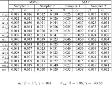
TABLE I
NMSES FOR THEESTIMATEDHYPERPARAMETERSUSING THEMMSE
ANDMAP ESTIMATORS
Fig. 1. Examples of empirical approximation (left) and detail (right) his-tograms and pdfs of frame coefficients corresponding to a synthetic image.
from 30 Monte Carlo runs. The NMSEs computed for the esti-mators associated with the two samplers of Sections IV-A and IV-B are reported in Table I. Table I shows that the proposed algorithms (using Sampler 1 of Section IV-A and Sampler 2 of Section IV-B) provide accurate estimates of the hyperparameters using the MMSE or the MAP estimator (with a slightly better performance for the MMSE estimator). The two samplers per-form similarly for this experiment. However, one advantage of Sampler 2 is that it can be applied to different kinds of redundant frames, unlike Sampler 1. Indeed, as reported in Section IV-A, the conditional distribution (13) is generally difficult to sample when the FR is not a union of orthonormal bases.
To further illustrate the good performance of the proposed estimator, Fig. 1 shows two examples of empirical histograms of wavelet frame coefficients (corresponding to ) that are in good agreement with the corresponding pdfs obtained after re-placing the hyperparameters by their estimates.
2) Example 2: In this experiment, another FR is considered, namely a tight frame version of the translation invariant wavelet transform [50] with Daubechies filters of length 8. The norm is also used for in (3) with . We use the same process to generate frame coefficients as for Example 1. The coefficients in each subband (i.e., each group) are modeled with the same values of the hyperparameters and , the number of groups being equal to 7. The same priors for the hyperparam-eters and as for Example 1 are used.
After generating the hyperparameters and frame coefficients, the hyperparameters are then sampled using the proposed
TABLE II
NMSES FOR THEESTIMATEDHYPERPARAMETERSUSING THEMMSE
ANDMAP ESTIMATORSWITHSAMPLER2
TABLE III
NMSES FOR THEESTIMATEDHYPERPARAMETERSUSING THEMMSE
ANDMAP ESTIMATESWITHSAMPLER2
algorithm, and estimated using the MMSE estimator. Table II shows NMSEs based on reference values of each hyperpa-rameter, where the frame coefficient vector is denoted by . Note that Sampler 1 is difficult to be implemented in this case because of the used frame properties. Consequently, only NMSE values for Sampler 2 have been reported in Table II.
3) Example 3: A third frame is considered in this experiment to show the versatility of our approach with respect to the choice of the FR: the contourlet transform [12] with Ladder filters over two resolution levels. The norm is used for in (3) with . We use the same procedure to generate frame coef-ficients as for Examples 1 and 2. The coefcoef-ficients in each of the eight groups are modeled with the same values of the hyperpa-rameters and and the same hyperparameter priors. After generating the hyperparameters and frame coefficients, the hy-perparameters are then supposed unknown and estimated using the MMSE estimator based on samples drawn with Sampler 2. Table III shows NMSEs based on reference values of each hy-perparameter.
B. Convergence Results
To be able to automatically stop the simulated chain and ensure that the last simulated samples are appropriately dis-tributed according to the posterior distribution of interest, a convergence monitoring technique based on the potential scale reduction factor (PSRF) is used by simulating several chains in parallel (see [51] for more details). This convergence monitoring technique indicates that sample convergence arises as soon as PSRF . Using the union of two orthonormal bases as a FR, Figs. 2 and 3 illustrate the variations w.r.t. the iteration number of the NMSE between the MMSE estimator and a reference estimator (computed by using a large number of burn-in and computation iterations, so as to guarantee that convergence has been achieved). The NMSE plots show that
Fig. 2. NMSE between the reference and current MMSE estimators w.r.t. iter-ation number corresponding to in .
Fig. 3. NMSE between the reference and current MMSE estimators w.r.t. iter-ation number corresponding to in .
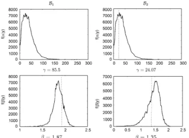
Fig. 4. Ground truth values (dashed line) and posterior distributions (solid line) of the sampled hyperparameters! and ", for the subbands # and# in and , repectively.
convergence is reached after about 150,000 iterations (burn-in period of 100,000 iterations), which corresponds to about 4 hours of computational time using Matlab 7.7 on an Intel Core 4–3 GHz architecture. When comparing the two proposed samplers in terms of convergence speed, it turns out from our simulations that Sampler 1 shows faster convergence than Sampler 2. Indeed, Sampler 1 needs about 110,000 iterations to converge, which reduces the global computational time to about 3 hours.
The posterior distributions of the hyperparameters and related to the subbands and in and are shown in Fig. 4, as well as the known original values. It is clear that the modes of the posterior distributions are around the ground truth
value, which confirms the good estimation performance of the proposed approach.
Note that when the resolution level increases, the number of subbands also increases, which leads to a higher number of hy-perparameters to be estimated and a potential increase of the re-quired computational time to reach convergence. For example, when using the union of two orthonormal wavelet bases with two resolution levels, the number of hyperparameters to esti-mate is .
C. Application to Image Denoising
1) Example 1: In this experiment, we are interested in re-covering an image (the Boat image of size 256 256 coded at 8 bpp) from its noisy observation affected by a noise uni-formly distributed over the ball with . We recall that the observation model for this image denoising problem is given by (3). The noisy image in Fig. 5(b) is simu-lated using the available reference image in Fig. 5(a) and the noise properties described above.
The union of two 2D separable wavelet bases and using Daubechies and shifted Daubechies filters of length 8 and 4 (as for validation experiments in Section V-A) is used as a tight FR. Denoising is performed using the MMSE esti-mator denoted as computed from sampled wavelet frame co-efficients. The adjoint frame operator is then applied to recover the denoised image from its denoised estimated wavelet frame coefficients . The obtained denoised image is de-picted in Fig. 5(d). For comparison purpose, the denoised image using a variational approach [52], [53] based on a MAP crite-rion using the estimated values of the hyperparameters with our approach is illustrated in Fig. 5(c). This comparison shows that, for denoising purposes, the proposed method gives better visual quality than the other reported methods. Signal-to-noise ratio and structural similarity (SSIM) [54] values are also given in Table IV to quantitatively evaluate denoising performance. Additional comparisons with respect to Wiener filtering and the algorithm developed in [36] (denoted here by SLR) are given in this table. Note that SLR can be applied only when the employed frame is the union of orthonormal bases, while our approach remains valid for any FR. Note also that SLR and Wiener filtering are basically de-signed to deal with Gaussian noise. This comparison shows that assuming the right noise model is essential to achieve good de-noising performance. On the other hand, comparisons with the variational approach, which accounts for the right uniform noise model and uses the same FR and coefficient groups, show that the improvement achieved by our algorithm is not only due to the model choice. The SNR and SSIM values are given for two additional test images ( Sebal and Tree) with different textures and contents to better illustrate the good performance of the pro-posed approach and its robustness to model mismatch. The cor-responding original, noisy and denoised images are displayed in Figs. 6 and 7.
It is worth noticing that the visual quality and quantitative results show that the denoised image based on the MMSE estimator of the wavelet frame coefficients is better than the one obtained with the Wiener filtering or the variational approach.
Fig. 5. Original Boat image (a), noisy image (b), denoised images using a vari-ational approach (c) and the proposed MMSE estimator (d).
TABLE IV
SNRANDSSIM VALUES FOR THENOISY ANDDENOISEDIMAGES
For the latter approach, it must be emphasized that the choice of the hyperparameters always constitute a delicate problem, for which our algorithm brings a numerical solution. Note also that compared with the variational approach, our algorithm recovers sharper and better denoised edges. However, our approach seems to be less performant in smooth regions, even if it does not introduce blurring effects like the variational approach.
In contrast with Wiener filtering and the variational approach which are very fast, SLR and our approach are more time-con-suming. Table V gives the iteration numbers and computational times for the used methods on an Intel Core 4–3 GHz architec-ture using a Matlab implementation. However, a high gain in computational time can be expected through code optimization and parallel implementation using multiple CPU cores. In fact, since the frame coefficients are split into groups with a couple of hyperparameters for each of them, a high number of loops is required, which is detrimental to the computational time in a Matlab implementation.
2) Example 2: In this experiment, we are interested in re-covering an image (the Straw image of size 128 128 coded at 8 bpp) from its noisy observation affected by a noise uniformly distributed over the centered ball of radius
Fig. 6. Original 1282 128 Sebal image (a), noisy image (b), denoised images using a variational approach (c) and the proposed MMSE estimator (d).
Fig. 7. Original 1282 128 Tree image (a), noisy image (b), denoised images using a variational approach (c) and the proposed MMSE estimator (d).
TABLE V
COMPUTATIONALTIME(INMINUTES)FOR THEUSEDMETHODS
when . Experiments are conducted using two dif-ferent FRs: the translation invariant wavelet transform with a
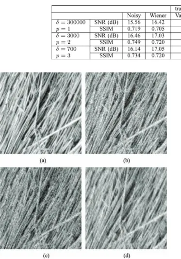
TABLE VI
SNRANDSSIM VALUES FOR THENOISY ANDDENOISEDSTRAWIMAGES
Fig. 8. Original Straw image (a), noisy image (b) and denoised images using the variational approach (c) and the proposed MMSE estimator (d).
Symmlet filter of length 8 and the contourlet transform with Ladder filters, both over 3 resolution levels. The norm was used for in (3). Figs. 8(a) and 8(b) show the original and noisy images using a uniform noise over the ball of radius 3000. When using the translation invariant wavelet transform, Figs. 8(c) and 8(d) illustrate the results generated by the denoising strategies based on the variational approach and the MMSE estimator using frame coefficients sampled with our algorithm. Table VI shows the SNR and SSIM values for noisy and denoised images using the pro-posed MMSE estimator for different values of and . This second set of image denoising experiments shows that the pro-posed approach performs well when using different kinds of FRs and various noise properties, which emphasizes its robust-ness to modelling errors.
VI. CONCLUSION
This paper proposed a hierarchical Bayesian model for frame coefficient from a noisy observation of a signal or image of in-terest. The signal perturbation was modeled by introducing a bound on a distance between the signal and its observation. A hierarchical model based on this maximum distance property was then defined. This model assumed flexible GG priors for
the frame coefficients. Vague priors were assigned to the hy-perparameters associated with the frame coefficient priors. Dif-ferent sampling strategies were proposed to generate samples distributed according to the joint distribution of the parameters and hyperparameters of the resulting Bayesian model. The gen-erated samples were finally used for estimation purposes. Our validation experiments indicated that the proposed algorithms provide an accurate estimation of the frame coefficients and hy-perparameters. The good quality of the estimates was confirmed on statistical processing problems in image denoising. Clearly, the proposed Bayesian approach outperforms the other methods because it allows us to use the right noise model and an appro-priate frame coefficient prior. The numerous experiments which were conducted also showed that the proposed algorithm is ro-bust to model mismatch. The hierarchical model studied in this paper assumed GG priors for the frame coefficients. However, the proposed algorithm might be generalized to other classes of prior models. Another direction of research for future work would be to extend the proposed framework to situations where the observed signal is degraded by a linear operator.
APPENDIX
SAMPLING ON THEUNIT BALL
This appendix explains how to sample vectors in the unit ball of . First, it is interesting to note that sam-pling on the unit ball can be easily performed in the particular case , by sampling independently along each space co-ordinate according to a distribution on the interval . Thus, this appendix focuses on the more difficult problem associated with a finite value of . In the following, denotes the norm. We recall the following theorem:
Theorem A.1 [55]: Let be the
random vector of i.i.d. components which have the following pdf
(24)
Let . Then, the random vector is uniformly distributed on the surface of the unit sphere of and the joint pdf of is
where and .
The uniform distribution on the unit sphere of will be denoted by . The construction of a random vector distributed within the ball of with can be derived from Theorem A.1 as expressed.
Theorem A.2 [55]: Let .
For every , the pdf of is given by
(26) In particular, if and , we obtain the uniform distribution on the unit ball of .
Sampling from a distribution on an ball of radius is straightforwardly deduced by scaling .
ACKNOWLEDGMENT
One of the authors (J.-C. Pesquet) would like to thank Prof. C. Vignat for some fruitful discussions.
REFERENCES
[1] H. Kawahara, “Signal reconstruction from modified auditory wavelet transform,” IEEE Trans. Signal Process., vol. 41, no. 12, pp. 3549–3554, Dec. 1993.
[2] L. Chaâri, J.-C. Pesquet, A. Benazza-Benyahia, and P. Ciuciu, “Auto-calibrated parallel MRI reconstruction in the wavelet domain,” in IEEE
Int. Symp. on Biomed. Imag. (ISBI), Paris, France, May 14–17, 2008, pp. 756–759.
[3] E. L. Miller, “Efficient computational methods for wavelet domain signal restoration problems,” IEEE Trans. Signal Process., vol. 47, no. 2, pp. 1184–1188, Apr. 1999.
[4] C. Chaux, P. L. Combettes, J.-C. Pesquet, and V. Wajs, “A for-ward-backward algorithm for image restoration with sparse represen-tations,” in Signal Process. Adaptat. Sparse Structured Represent., Rennes, France, Nov. 2005, pp. 49–52.
[5] M. B. Martin and A. E. Bell, “New image compression techniques using multiwavelets and multiwavelet packets,” IEEE Trans. Image
Process., vol. 10, no. 4, pp. 500–510, Apr. 2001.
[6] M. De Meuleneire, “Algebraic quantization of transform coefficients for embedded audio coding,” in Proc. IEEE Int. Conf. Acoust., Speech,
Signal (ICASSP), Las Vegas, NV, Apr. 4, 2008, pp. 4789–4792. [7] S. Mallat, A Wavelet Tour of Signal Processing. New York:
Aca-demic, 1999.
[8] R. Coifman, Y. Meyer, and V. Wickerhauser, “Wavelet analysis and signal processing,” in Wavelets and Their Applications. Boston, MA: Jones & Bartlett, 1992, pp. 153–178.
[9] S. Mallat, “Geometrical grouplets,” Appl. Comput. Harm. Anal., vol. 26, no. 2, pp. 161–180, 2009.
[10] E. J. Candès and D. L. Donoho, “Recovering edges in ill-posed inverse problems: Optimality of curvelet frames,” Ann. Stat., vol. 30, no. 3, pp. 784–842, 2002.
[11] F. Destrempes, J.-F. Angers, and M. Mignotte, “Fusion of hidden Markov random field models and its Bayesian estimation,” IEEE
Trans. Image Process., vol. 15, no. 10, pp. 2920–2935, Oct. 2006. [12] M. N. Do and M. Vetterli, “The contourlet transform: An efficient
di-rectional multiresolution image representation,” IEEE Trans. Image
Process., vol. 14, no. 12, pp. 2091–2106, Dec. 2005.
[13] E. Le Pennec and S. Mallat, “Sparse geometric image representations with bandelets,” IEEE Trans. Image Process., vol. 14, no. 4, pp. 423–438, Apr. 2005.
[14] C. Chaux, L. Duval, and J.-C. Pesquet, “Image analysis using a dual-tree m-band wavelet transform,” IEEE Trans. Image Process., vol. 15, no. 8, pp. 2397–2412, Aug. 2006.
[15] M. Seeger, S. Gerwinn, and M. Bethge, “Bayesian inference for sparse generalized linear models,” Mach. Learn., vol. 4701, pp. 298–309, Sep. 2007.
[16] A. B. Watson, G. Y. Yang, J. A. Solomon, and J. Villasenor, “Visibility of wavelet quantization noise,” IEEE Trans. Image Process., vol. 6, no. 8, pp. 1164–1175, Aug. 1997.
[17] Y. Zhang, A. O. Hero, and W. L. Rogers, “A bounded error estima-tion approach to image reconstrucestima-tion,” in Proc. Nucl. Sci. Symp. Med.
Imag. Conf., Orlando, FL, Oct. 1992, pp. 966–968.
[18] S. Rangan and V. K. Goyal, “Recursive consistent estimation with bounded noise,” IEEE Trans. Inf. Theory, vol. 47, no. 1, pp. 457–464, Jan. 2001.
[19] T. M. Breuel, “Finding lines under bounded error,” Pattern Recogn., vol. 29, no. 1, pp. 167–178, Jan. 1996.
[20] M. Alghoniemy and A. H. Tewfik, “A sparse solution to the bounded subset selection problem: A network flow model approach,” in Proc.
IEEE Int. Conf. Acoust., Speech, Signal (ICASSP), Montreal, Canada, May 17–21, 2004, pp. 89–92.
[21] C. Robert and G. Castella, Monte Carlo Statistical Methods. New York: Springer, 2004.
[22] O. Cappé, “A Bayesian approach for simultaneous segmentation and classification of count data,” IEEE Trans. Signal Process., vol. 50, no. 2, pp. 400–410, Feb. 2002.
[23] C. Andrieu, P. M. Djuric, and A. Doucet, “Model selection by MCMC computation,” Signal Process., vol. 81, pp. 19–37, Jan. 2001. [24] M. Ichir and A. Mohammad-Djafari, “Wavelet domain blind image
separation,” in Proc. SPIE Tech. Conf. Wavelet Appl. Signal and Image
Process. X, San Diego, CA, Aug. 2003.
[25] A. Jalobeanu, L. Blanc-Féraud, and J. Zerubia, “Hyperparameter esti-mation for satellite image restoration using a MCMC maximum likeli-hood method,” Pattern Recogn., vol. 35, no. 2, pp. 341–352, Nov. 2002. [26] S. Makni, P. Ciuciu, J. Idier, and J.-B. Poline, “Joint detection-estima-tion of brain activity in funcdetection-estima-tional MRI: A multichannel deconvoludetection-estima-tion solution,” IEEE Trans. Signal Process., vol. 53, no. 9, pp. 3488–3502, Sep. 2005.
[27] N. Dobigeon, A. O. Hero, and J.-Y. Tourneret, “Hierarchical Bayesian sparse image reconstruction with application to MRFM,” IEEE Trans.
Image Process., vol. 19, no. 9, pp. 2059–2070, Sep. 2009.
[28] T. Blumensath and M. E. Davies, “Monte Carlo methods for adaptive sparse approximations of time-series,” IEEE Trans. Signal Process., vol. 55, no. 9, pp. 4474–4486, Sep. 2007.
[29] S. Zeger and R. Karim, “Generalized linear models with random effects a Gibbs sampling approach,” J. Amer. Statist. Assoc., vol. 86, no. 413, pp. 79–86, Mar. 1991.
[30] L. Tierney, “Markov chains for exploring posterior distributions,” Ann.
Stat., vol. 22, no. 4, pp. 1701–1762, 1994.
[31] W. K. Hastings, “Monte Carlo sampling methods using markov chains and their applications,” Biometrika, vol. 57, pp. 97–109, 1970. [32] S. Geman and D. Geman, “Stochastic relaxation, Gibbs distribution and
the Bayesian restoration of image,” IEEE Trans. Pattern Anal. Mach.
Intell., vol. 6, pp. 721–741, 1984.
[33] D. Leporini and J.-C. Pesquet, “Bayesian wavelet denoising: Besov priors and non-Gaussian noises,” Signal Process., vol. 81, no. 1, pp. 55–67, Jan. 2001.
[34] P. Mueller and B. Vidakovic, “MCMC methods in wavelet shrinkage: Non-equally spaced regression, density and spectral density estima-tion,” in Bayesian Inference in Wavelet-Based Models, P. Mueller and B. Vidakovic, Eds. New York: Springer, 1999, pp. 187–202. [35] G. Heurta, “Multivariate Bayes wavelet shrinkage and applications,” J.
Appl. Statist., vol. 32, no. 5, pp. 529–542, Jul. 2005.
[36] C. Févotte and S. J. Godsill, “Sparse linear regression in unions of bases via Bayesian variable selection,” IEEE Signal Process. Lett., vol. 13, no. 7, pp. 441–444, Jul. 2006.
[37] P. J. Wolfe and S. J. Godsill, “Bayesian estimation of time-frequency coefficients for audio signal enhancement,” in Adv. Neural Inf. Process.
Syst., 2003, vol. 15, pp. 1197–1204.
[38] M. Kowalski and B. Torrésani, “Random models for sparse signals ex-pansion on unions of bases with application to audio signals,” IEEE
Trans. Signal Process., vol. 56, no. 8, pp. 3468–3481, Aug. 2008. [39] S. Molla and B. Torrésani, “A hybrid scheme for encoding audio signal
using hidden Markov models of waveforms,” Appl. Comput. Harmon.
Anal., vol. 18, no. 2, pp. 137–166, Mar. 2005.
[40] D. L. Donoho, “Denoising by soft-thresholding,” IEEE Trans. Inf.
Theory, vol. 41, no. 3, pp. 613–627, May 1995.
[41] S. G. Mallat, “A theory for multiresolution signal decomposition: The wavelet representation,” IEEE Trans. Pattern Anal. Mach. Intell., vol. 11, no. 7, pp. 674–693, 1989.
[42] R. L. Joshi, H. Jafarkhani, J. H. Kasner, T. R. Fischer, N. Farvardin, M. W. Marcellin, and R. H. Bamberger, “Comparison of different methods of classification in subband coding of images,” IEEE Trans. Image
Process., vol. 6, no. 11, pp. 1473–1486, Nov. 1997.
[43] E. P. Simoncelli and E. H. Adelson, “Noise removal via Bayesian wavelet coring,” in IEEE Int. Conf. on Image Process. (ICIP), Lau-sanne, Switzerland, Sep. 16–19, 1996, pp. 379–382.
[44] P. Moulin and J. Liu, “Analysis of multiresolution image denoising schemes using generalized-Gaussian priors,” in Proc. IEEE-SP Int.
Symp. Time-Frequency Time-Scale Analysis, Pittsburgh, PA, Oct. 1998, pp. 633–636.
[45] M. N. Do and M. Vetterli, “Wavelet-based texture retrieval using gen-eralized Gaussian density and Kullback-Leibler distance,” IEEE Trans.
Image Process., vol. 11, no. 2, pp. 146–158, Feb. 2002.
[46] M. W. Seeger and H. Nickisch, “Compressed sensing and bayesian experimental design,” in Int. Conf. Mach. Learn., Helsinki, Finland, Jul. 5–9, 2008, pp. 912–919.
[47] S. D. Babacan, R. Molina, and A. K. Katsaggelos, “Fast Bayesian compressive sensing using Laplace priors,” in Proc. IEEE Int. Conf.
Acoust., Speech, Signal (ICASSP), Taipei, Taiwan, Apr. 19–24, 2009, pp. 2873–2876.
[48] H. Jeffreys, “An invariant form for the prior probability in estimation problems,” Proc. Royal Soc. London. Series A, vol. 186, no. 1007, pp. 453–461, 1946.
[49] N. Dobigeon and J.-Y. Tourneret, “Truncated multivariate Gaussian distribution on a simplex,” Univ. Toulouse, France, Tech. rep., Jan. 2007.
[50] R. Coifman and D. Donoho, “Translation-invariant de-noising,” in
Wavelets and Statistics. New York: Springer, 1995, vol. 103, Lecture Notes in Statistics, pp. 125–150.
[51] A. Gelman and D. B. Rubin, “Inference from iterative simulation using multiple sequences,” Statist. Sci., vol. 7, no. 4, pp. 457–472, Nov. 1992.
[52] C. Chaux, P. L. Combettes, J.-C. Pesquet, and V. R. Wajs, “A varia-tional formulation for frame-based inverse problems,” Inv. Problems, vol. 23, no. 4, pp. 1495–1518, Aug. 2007.
[53] P. L. Combettes and J.-C. Pesquet, “A proximal decomposition method for solving convex variational inverse problems,” Inv. Problems, vol. 24, no. 4, p. 27, Nov. 2008.
[54] Z. Wang, A. C. Bovik, H. R. Sheikh, and E. P. Simoncelli, “Image quality assessment: From error visibility to structural similarity,” IEEE
Trans. Image Process., vol. 13, no. 4, pp. 600–612, Apr. 2004. [55] A. K. Gupta and D. Song, “Lp-norm uniform distribution,” J. Statist.
Plann. Inference, vol. 125, no. 2, pp. 595–601, Feb. 1997.
Lotfi Chaâri(S’08) was born in Sfax, Tunisia, in 1983. He received the en-gineering and master degrees in telecommunication from the École Supérieure des Communications (SUP’COM), Tunis, Tunisia in 2007.
He is currently pursuing the Ph.D. degree in 2008 with Professor J.-C. Pesquet at the Laboratoire d’Informatique (UMR-CNRS 8049) of the Uni-versité Paris-Est Marne-la-Vallée. His research is focused on Bayesian and variational approaches for image processing and their application to parallel MRI reconstruction.
Jean-Christophe Pesquet(S’89–M’91–SM’99) received the engineering de-gree from Supélec, Gif-sur-Yvette, France, in 1987, the Ph.D. dede-gree from the
Université Paris-Sud (XI), Paris, France, in 1990, and the Habilitation à Diriger des Recherches from the Université Paris-Sud in 1999.
From 1991 to 1999, he was a Maître de Conférences at the Université Paris-Sud, and a Research Scientist at the Laboratoire des Signaux et Systèmes, Centre National de la Recherche Scientifique (CNRS), Gif sur Yvette. He is currently a Professor with Université Paris-Est Marne-la-Vallée, France, and a Research Scientist with the Laboratoire d’Informatique of the university (UMR-CNRS 8049).
Jean-Yves Tourneret(SM’08) received the ingénieur degree in electrical en-gineering from the École Nationale Supérieure d’Électronique, d’Électrotech-nique, d’Informatique et d’Hydraulique of Toulouse (ENSEEIHT), France, in 1989 and the Ph.D. degree from the National Polytechnic Institute, Toulouse, in 1992.
He is currently a professor with the University of Toulouse (ENSEEIHT), France and a member of the IRIT laboratory (UMR 5505 of the CNRS). His research activities are centered around statistical signal processing with a par-ticular interest to Markov chain Monte Carlo methods.
Dr. Tourneret was the Program Chair of the European Conference on Signal Processing (EUSIPCO), held in Toulouse in 2002. He was also member of the Organizing Committee for the International Conference ICASSP’06 held in Toulouse in 2006. He has been a member of different technical committees including the Signal Processing Theory and Methods (SPTM) Committee of the IEEE Signal Processing Society (2001–2007 and 2010-present). He is cur-rently serving as an Associate Editor for the IEEE TRANSACTIONS ONSIGNAL
PROCESSING.
Philippe Ciuciu(M’02) was born in France in 1973. He graduated from the École Supérieure d’Informatique Électronique Automatique, Paris, France, in 1996. He received the DEA and Ph.D. degrees in signal processing from the Université de Paris-sud, Orsay, France, in 1996 and 2000, respectively.
In November 2000, he joined the fMRI Signal Processing Group as a Post-doctoral Fellow with Service Hospitalier Frédéric Joliot (CEA, Life Science Di-vision, Medical Research Department) in Orsay, France. Since November 2001, he has been a permanent CEA Research Scientist. In 2007, he moved to Neu-roSpin, an ultrahigh magnetic field center in the LNAO lab. Currently, he is Principal Investigator of the Neurodynamics Program in collaboration with A. Kleinschmidt (DR INSERM) at the Cognitive Neuroimaging Unit (INSERM/ CEA U562). His research is focused on the application of statistical methods (e.g., Bayesian inference, model selection), stochastic agorithms (MCMC), and wavelet-based regularized approaches to functional brain imaging (fMRI) and to parallel MRI reconstruction.
Amel Benazza-Benyahiareceived the engineering degree from the National Institute of Telecommunications, Evry, France, in 1988, the Ph.D. degree from the Université Paris-Sud (XI), Paris, France, in 1993, and the Habilitation Uni-versitaire from the Ecole Supérieure des Communications (SUP’COM), Tunis, Tunisia, in 2003.
She is currently a Professor with the Department of Applied Mathematics, Signal Processing and Communications, SUP’COM. She is also a Research Sci-entist with the Unité de Recherche en Imagerie Satellitaire et ses Applications (URISA), SUP’COM. Her research interests include multispectral image com-pression, signal denoising, and medical image analysis.