Impedance active control of flight control devices

To c

Ced

Inte

Mon

This

Epri

Any

adm

cite this

dric. Imp

ernationa

ntréal, C

s is an

ints ID: 3

y corresp

ministrato

docume

pedance

al Confe

Canada.

author-d

3914

pondence

or:

staff-o

ent:

DEF

e active c

erence on

deposited

e concer

oatao@in

FAY Fra

control o

n Advan

d version

rning thi

np-toulo

ancois, A

of flight

nced Inte

n publis

is servic

use.fr

ALAZAR

control d

elligent M

shed in:

ce should

RD Dani

devices.

Mechatro

http://oa

d be sen

iel, ANT

In: 2010

onics , 0

atao.univ

nt to the

TRAYGU

0 IEEE/A

06-09 Jul

v-toulous

e reposito

UE

/ASME

l 2010,

se.fr/

ory

Impedance Active control of flight control devices

Francois Defa¨y, Daniel Alazard

Universit´e de Toulouse - ISAE

Toulouse, France

C´edric Antraygue

Ratier-Figeac

Figeac, France

Abstract— The work presented in this paper concerns the active control of flight control devices (sleeves, yokes, side-sticks, rudder pedals , ...). The objective is to replace conventional technologies by active technology to save weight and to feedback kinesthetic sensations to the pilot. Some architectures are proposed to control the device mechanical impedance felt by pilot and to couple pilot and co-pilot control devices. A first experimental test-bed was developed to validate and illustrate control laws and theirs limitations due to dynamic couplings with the pilot own-impedance.

I. INTRODUCTION

In the past, pilots used their own physical strength to pilot aircraft since their yokes and rudder pedals were directly connected to control surfaces by cables. Therefore, the pilot felt exactly what happened during the flight. Gradually, the performance and the size of aircraft increased, hydraulic actuators were added to the aircraft’s control systems. This hardware facilitated the piloting, especially after the advent of digital control systems. Thus, the pilot acts no more directly on the control surfaces; onboard computers and avionics operate between the pilot and control surfaces deflections. It is true that this technology brings greater accuracy, security, comfort and makes the flight more enjoyable. However, the pilot has now lost the feeling provided by traditional devices.

To overcome this problem, an active device with force feedback can be used to control the mechanical impedance felt by the pilot. Such an active device can be used also to feedback kinesthetic sensations to the pilot according to the operational state of the aircraft. It is also important to note that the introduction of this technology can actively generate significant gains in terms of mass, volume, assembly time and number of modules to be installed as shown in Fig. 1. This technology can be used to couple pilot and co-pilot control devices removing mechanical links between them.

This work has strong links with human-machine interfaces (HMI) [4], [9], [10] and [11], tele-operation [5] and [7] in medical or nuclear fields, automotive industry (steer-by-wire [2], [3] and [16]) and more generally in the context of haptic interfaces.

Haptic interfaces:

The word haptic comes from the Greek word haptein which means touch. It is defined by ”on the skin sensitivity” and ”scientific study of touch.” In practice, the term haptic is used to refer to two types of sensory feedbacks: the force or kinesthetic feedback and tactile feedback. The first relates

to the perception of contact forces, hardness, weight and inertia of an object. This type of return acts on the operator movements and solicits muscles, tendons and joints. The tactile feedback, in turn, concerns the perception of surface (roughness, texture), temperature shifts and detection of edges [4]. In a general way, the integration of haptic feedback includes several steps: one must first master the control of the actuator, which represents the most inner loop; then, the highest level control loop design, eg at the end effector (the control device). And finally, to create a virtual environment able to simulate physical phenomena and to provide artificial sensations associated with these physical phenomena to the user (the operator).

The overall aim of the project is to control the mechanical impedance of the control device in order to:

• adjust the impedance to the morphology of the pilot

• feedback kinesthetic sensations to the pilot in order to

advise on the operational state of the aircraft (eg: near the boundaries of the flight envelope)

• coupling pilot and copilot yokes,

• assess the impact of such a system on human factors

(tolerance to defects, pilot fatigue, . . . ).

An experimental test bed, composed of two identical and active yokes, was developed to illustrate various control con-cepts. In this paper the control of the mechanical impedance of each yoke and the coupling of pilot and copilot yokes

Electric Motor Electric Control Friction device

device with a spring trim actuator fill au-topilot mode

Shock

17 module, 11 connecting rods, 8 cables Old techology

4 module, 3 connecting rods Active techology Fig. 1. Controls assets and liabilities to an aircraft

are particularly considered: the required stiffness for the pilot-copilot yokes coupling and the mechanical impedance reduction of each yoke are antagonist specifications. This is the specific feature of this application which is not addressed in previous works in the field of tele-operation or steering by wire. In [17], two complementary control architecture was proposed to control the mechanical impedance of each yoke. The first one (also called maximal impedance ap-proach) involves a very stiff inner angular position servo-loop and an outer servo-loop feedbacking the measured torque to the position input reference through the admittance reference model. The second one (also called maximal admittance approach) involves an inner torque servo-loop and an outer loop feedbacking the yoke angular position to the torque input reference through the impedance reference model. In this paper the first approach is considered to simply couple pilot and co-pilot yokes. This solution is validated on the experimental test-bed. Experimental tests highlight some dynamic couplings with the pilot own-impedance which depends on the way the pilot holds the yoke.

The article is structured as follows:

In Section II, the model of the experimental test-bed and the control objectives are presented. In section III, the maximal impedance approach is presented and used to coupled pilot and co-pilot yokes. Experimental results are presented in section IV with a particular focus on the destabilizing cou-pling with pilot own-impedance when the pilot tightens the yoke firmly. Maximal admittance approach is summarized in appendix.

II. MODEL AND OBJECTIVES

The experimental test-bed is depicted in Fig. 2 and is composed of two identical and active yokes. Each active yoke is composed of:

• a motor applying a torqueC_m. Its inertia is denotedJ_m

and its angular position θ_mis measured by a resolver,

• a gear box (gear ratio is 100),

• a torque-meter C_mes. The strain torsion gauge

intro-duces a stiffnessk (with a small damping coefficient f)

in the transmission,

• the steering wheel whose inertia is denoted J_y and

position θ_y is measured by a resolver. The manual

torque applied by the pilot on this yoke is denotedC_y.

Remarks: in the sequel all parameters and variables are ex-pressed from the gear output side (slow side). The exponent p and c will refer respectively to the pilot and the co-pilot yoke, respectively.

In [17] a detailed model of the active yoke and its transmission is presented. The simplified string-inertia model

presented in Fig. 3 is considered here. The 4-th order

model G(s) between the 2 inputs C_y and C_m and the 3

outputsθ_y,θ_mandC_mesis described by the following state

Control Unit

Copilot yoke Pilot yoke Real Time PC

Fig. 2. Active yoke demonstrator

representation: ˙x =     0 0 1 0 0 0 0 1 −k Jy k Jy −f Jy f Jy k Jm −k Jm f Jm −f Jm    x +     0 0 0 0 1 Jy 0 0 1 Jm    u y =   1 0 0 0 0 1 0 0 k −k 0 0  x (1) with: x = [θyθm ˙θy ˙θm]T, u = [CyCm]T, y = [θy θmCmes] . θm θy Cy Cm k f Cmes Jm Jy

Fig. 3. Simplified mechanical model test

Some experiments have been carried to identify these parameters:

• k = 800N.m/rad, f = 1.28 Nm/(rad/s)

• Jm= 8.7.10−2kg.m2;J_y = 2.3.10−2kg.m2.

Finally the sampling periodT_s= 0.0025 s is chosen as low

as possible, the limitation comes from the torque sensor.

Gd(z) is the continuous to discrete-time conversion of G(s)

assuming zero-order holds (ZOH) on the inputs ofG(s) and

G(i : j, k : l) is the sub-system of G(s) restricted to inputs k to l and outputs i to j.

The dynamics of this system is characterized by a

rigid mode and a flexible mode with a pulsation ω_f =

p

k(Jm+ Jy)/Jm/Jy = 210 rad/s and a very low

damp-ing ratio (ξ = 0.08).

From the single yoke control point of view, the objective (objective #1) is to shape the yoke mechanical impedance

in order to meet a reference impedance modelZ_ref(s). The

impedanceZ_y(s) felt by the pilot is defined as the transfer

between the steering wheel positionθ_y and the pilot torque

Cy such that Z_y(s) = C_θy

model is defined by:Z_ref(s) = J_a.s2+ D_a.s + K_a where

Ja,D_aandK_aare respectively the apparent inertia, damping

and stiffness of the yoke. One can also define the mechanical

admittance as the inverse of the impedance Y (s) = _Z(z)1 .

Admittance have the interest to be a strictly proper transfer. The control design will be as much more efficient than it will allow a large reference impedance range (that is: a

large range on parametersJ_a,D_a andK_a) to be taken into

account.

From the pilot/copilot yokes couplings point of view, the objective (objective #2) is to minimize the frequency domain

response R(ω) of the 2 × 1 transfer between the pilot and

copilot torques[C_yp, C_yc]T and the 2 yokes relative position

θp

y−θcy.

III. FEEDBACKCONTROL SCHEME

The discrete-time control architecture involving pilot and copilot yoke models is depicted on Fig. 4.

Pilot Yoke Gp_(s) Cc mes θp y Cp mes θp m ZoH Position Servo Loop Cθ(z) Cp y

Y

Y

Fig. 4. Control architecture based on the maximal impedance approach Gp+c_cl .

This architecture involves, for each yoke:

• an inner position servo-loop through the controller

Cθ(z),

• an outer feedback between the sum of pilot and copilot

measured torques (C_mesp +C_mesc ) and the position input

referenceθ_refi , through the admittance reference model

Yi

ref(z) (i = p, c). Yrefi (z) is obtained from Yrefi (s)

by a continuous to discrete time TUSTINconversion.

This solution is called maximal impedance solution (or minimal admittance solution) because the position servo loop is tuned very stiff in such way that if the position input

reference is set to 0 (i.e. Y_ref(s) = 0), then the position

servo-loop rejects external disturbances including the pilot

torqueC_y. Therefore the yoke seems to be strongly clamped

on its reference position i.e. the impedance is closed to infinite.

The servo-loop controllerC_θ(z) is the same for both yokes

and is defined by the following discrete-time transfer:

Ci m = Cθ(z)   θi y−θiref θi m Ci mes   (2) = [−Kp, −Kvz − 1_T sz , −Kc z − 1 Tsz ]   θi y−θiref θi m Ci mes  (3).

This servo-loop feedbacks:

• the tracking errorθi_y−θi_ref through a proportional gain

Kp,

• the motor angular rate through a gainK_v,

• the time-derivative of the measured torque C_mesi

through a gainK_c. One can note that _dtdC_mesi = ˙C_mesi

is proportional (through the stiffness k) to the relative

angular rate ˙θi_y− ˙θ_mi . This feedback allows the flexible

mode to be damped. Indeed, although ˙θ_m is collocated

with the actuator, the motor rate feedback (through the

gain K_v) does not damp the flexible mode enough

because this flexible mode is badly observable from ˙θi_m

as J_mis much greater than J_y.

Kp, K_v and K_c are tuned to maximize the closed-loop

flexible mode damping ratio and to increase the closed-loop rigid-mode bandwidth:

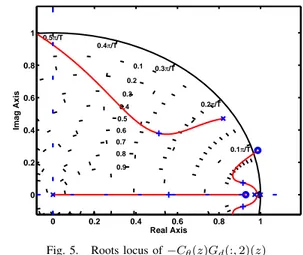
Kp = 150 Nm/rd; Kv= 4.5 Nms/rd, Kc= 0.013 s .

Such a tuning is highlighted by the root locus depicted in Fig. 5. 0 0.2 0.4 0.6 0.8 1 0 0.2 0.4 0.6 0.8 1 0.9 0.8 0.7 0.6 0.5 0.4 0.3 0.2 0.1 0.5π/T 0.4π/T 0.3π/T 0.2π/T 0.1π/T Real Axis Imag Axis

Fig. 5. Roots locus of −C_θ(z)G_d(:, 2)(z)

The yoke admittance Y_y(z) once the position loop is

closed (i.e: when Y_refi (z) = 0) is depicted in Fig. 7 (green

line) with the open-loop yoke impedance (blue line) and the impedance obtained by the maximal admittance approach (red line) (see appendix).

Inside the position servo loop bandwidth, it can shown

thatC_mes≈C_y(≈ −C_m). Then, objective #1 can be simply

met feedbacking the measured torque C_mes to the position

input referenceθ_ref through the admittance reference model

Yref. Of course, the magnitude of Y_ref is limited by the

outer loop stability. Qualitatively, this structure supports

any admittance modelY_ref whose low frequency response

is inside the area bounded by the minimal (green) and maximal (red) admittance responses in Fig. 7. For instance,

forY_ref(s) = 1/(0.025s2+ 0.22s + 1) (nominal admittance

reference model) that is: a quite weak apparent inertia and stiffness, the root locus of the outer loop in depicted in

Fig. 6. The obtained yoke admittance once the outer loop is closed is plotted in Fig. 7 (purple line) with the admittance

reference model Y_ref(s) (dashed purple line). The obtained

yoke admittance is very closed to the reference model.

0 0.2 0.4 0.6 0.8 1 0 0.2 0.4 0.6 0.8 1 0.9 0.8 0.7 0.6 0.5 0.4 0.3 0.2 0.1 0.5π/T 0.4π/T 0.3π/T 0.2π/T 0.1π/T Real Axis Imag Axis

Fig. 6. Roots locus of outer loop withYref(s) = 1/(0.025s2_+0.22s+1). To satisfy objective #2, a simple solution consists in feedbacking the sum of the pilot and copilot torques to the admittance reference model input of each yoke. Then, although each yoke seems very ”light” due to the choice of

Yref(s), the dynamic coupling between yokes is quite strong,

that is: the magnitude of the frequency responseR(ω) of the

coupling performance is very low (see Fig. 7, cyan plot).

Singular Values Frequency (rad/sec) Singular Values (dB) 10−1 100 101 102 103 104 −150 −100 −50 0 50 100

Fig. 7. Yoke admittance frequency-domain responses: open-loop (blue), minimal admittance or closed-loop withYref= 0 (green), maximal admit-tance (red), nominal admitadmit-tance reference modelYref(s) = 1/(0.025s2₊ 0.22s + 1) (dashed purple), closed loop with nominal admittance reference model (purple) and coupling performanceR(ω) (cyan).

IV. EXPERIMENTAL RESULTS A. Quasi-static impedance of the yoke

The first experiment consists to apply very low frequency

(≤ 1 rd/s) hand made solicitations to the yoke in order

to illustrate the quasi-static (or low frequency) impedance of the controlled yoke for various tuning. For the maximal impedance and maximal admittance tunings, the results are presented in Fig. 8 where the measured torque is plotted vs the yoke angular position:

• for the maximal impedance tuning (green plot),

one can compute the static admittance 0.15/21 =

0.007 rd/N/m (i.e. −43 dB) which was predicted by frequency-domain analysis presented in Fig. 7 (also the green plot),

• for the maximal admittance tuning (red plot), the

impedance is almost zero (according also to the frequency-response of 7). -0.2 0 0.2 0.4 0.6 0.8 1 1.2 -5 0 5 10 15 20 25

Yoke angular position (rad)

M e a s u re d t o rq u e ( N .m )

Fig. 8. Maximal (green) and minimal (blue) static impedances of the yoke (experimental responses).

B. Dynamic impedance of the yoke and pilot/copilot yokes coupling

The objective is now to highlight the dynamic coupling of pilot and co-pilot yokes. The manual solicitation is a

quasi-periodic signal fast enough (pulsation is around10 rd/s) on

the pilot yoke, the co-pilot yoke being free. The control law presented in Fig. 4 is tuned with the nominal impedance

reference model Y_ref(s) = 1/(0.025s2+ 0.22s + 1). The

results are presented in Fig. 9 for pilot and copilot angular positions and Fig. 10 for the pilot measured torque. The peak

to peak values are around1 Nm for the torque and 0.5 rd for

the position. Thus the theoretical value predicted on Fig. 7

(−6 dB at 10 rd/s, marked by a black diamond) is confirmed

by this experimental test. Although the yoke seems to be very light, the coupling between the pilot and co-pilot yokes

positions is very strong and the errorθp_y−θ_yc is quite small.

C. Dynamic coupling with pilot own-impedance

The control structure proposed in Fig.4 is very interesting because it allows a wide range of admittance reference model to be taken into account but works better for low admittances. For very high admittance reference models, some dynamic couplings with the pilot own impedance can destabilize the system. This behavior is highlighted by the experiment reported in Fig. 11 where, after a double square form maneuver (one can also appreciate the efficiency of pilot and co-pilot yokes couplings), the pilot tightens the

25 26 27 28 29 30 31 32 33 -0.3 -0.2 -0.1 0 0.1 0.2 0.3 0.4 Time (s) A n g u la r p o s it io n ( ra d ) θ_yp θc y θc y-θ p y

Fig. 9. Angular positions of pilotθ_ypandθ_yccopilot yokes when the pilot applies a periodic excitation on its yoke and the co-pilot yoke is free.

25 26 27 28 29 30 31 32 33 -1 -0.5 0 0.5 1 1.5 Time (s) P ilo t T o rq u e ( N .m )

Fig. 10. Measured torque on the pilot yoke when the pilot applies a periodic excitation on its yoke and the co-pilot yoke is free.

11 s). Then an unstable oscillation (around 4 Hz) appears till the motor current becomes too important and activates the security switch.

Although the torque is measured, the pilot cannot be con-sidered as a pure torque generator. The pilot own-impedance acts as an external feedback on the control device. Such a modeling of the human hand holding a yoke is not a trivial task but this dynamic coupling phenomenon can be analyzed

assuming the pilot introduces an inertiaJ_h, a dampingG_han

a stiffnessK_hacting as feedback gains between yoke angular

acceleration ¨θ_yp, rate ˙θ_ypand positionθ_yp, respectively, and the

pilot torque C_yp (with a negative feedback). Then one can

plot the corresponding root locus to analyze the destabilizing values for these 3 gains. This analysis is presented in Fig.12: one can notice that the system becomes unstable at low frequency for quite low values of these gains and one can

imagine that a combination of these 3 gainsJ_h,D_h andK_h

can explain the experimental instability encountered around 4 Hz.

For high admittance requirement, the maximal admittance

5 6 7 8 9 10 11 12 13 -0.8 -0.6 -0.4 -0.2 0 0.2 0.4 0.6 Time (s) Y o k e s a n g u la r p o s it io n s ( ra d ) θ y c θ_yp

Fig. 11. Measured torque on the pilot yoke when the pilot applies a periodic excitation on its yoke and the co-pilot yoke is free.

0.3 0.4 0.5 0.6 0.7 0.8 0.9 1 1.1 −0.1 0 0.1 0.2 0.3 0.4 0.9 0.8 0.7 0.6 0.5 0.1π/T Real Axis Imag Axis

Fig. 12. Analysis of un-stabilizing couplings with pilot own-impedance. Roots locus of closed-loop systemGp+c_cl between the pilot torqueC_ypand: (i) the yoke angular acceleration ¨θyp(blue locus; instability appears forJh= 0.045 Kgm2_{), (ii) the yoke angular rate ˙θ}p

y(red locus; instability appears forDh= 2.7 Nms/rd) and (iii) the yoke angular position θp_y(green locus; instability appears forK_h= 12Nm/rd.)

approach presented in appendix is more efficient and is more insensitive to the dynamics couplings with the pilot (co-pilot) own-impedance. But as a counterpart this approach is not suitable to strongly couple the pilot and copilot yokes (objective #2).

V. CONCLUSIONS AND FUTURE WORKS In this article two methods have been presented to control the mechanical impedance of a yoke. These methods are based on position and force servo-loops designed by con-ventional control design methods. The control design must take into account the flexible mode introduced by the torque-meter into the system and must be done in discrete-tome domain to quite representative of all dynamic phenomena. The maximal impedance method is more efficient for high impedance reference models and to couple pilot and copilot yokes. For low impedance, unstable dynamic couplings with pilot own-impedance were highlighted in experiments and analyzed.

Future works on this project will concern the use of robust and multi-variable methodologies to:

• take into account uncertainties in modeling of

bio-impedance [3] of the human operator,

• generalize the control design to multi-degree of

free-dom control devices (side-stick): the two methodologies proposed in this article are based on the analysis of graphical tools (root locus). This kind of approach is quite suitable for one degree of freedom systems. To deal with several degrees of freedom systems, a sys-tematic methodology is required, allowing controllers to be defined directly from desired impedance reference models.

REFERENCES

[1] D. Alazard et J.P. Chr´etien. Commande active des structures flexibles : applications a´eronautiques et spatiales. Notes de cours de SUPAERO, Toulouse, 2000.

[2] N. Bajc¸inca, R. Cortes˜ao, J. Bals, G. Hirzinger, M. Hauschild, Haptic Control for Steer-by-Wire Systems, Proceedings of the 2003 IEEE/RSJ Intl. Conference on lnielligent Robots and Systems, Las Vegas, Nevada, 2003.

[3] N. Bajc¸inca. Robust Control Methods with Applications to Steer-by-Wire Systems. PhD Thesis, Elektrotechnik und Informatik Technische Universit¨at Berlin, 2006.

[4] G. Casiez. Contribution `a l’´etude des interfaces haptiques. Le DigiHap-tic : un p´eriph´erique haptique de bureau `a degr´es de libert´e s´epar´es. Th`ese de Doctorat, Universit´e des Sciences et Technologies de Lille, 2004.

[5] J. E. Colgate, P. E. Grafing, M. C. Stanley, G. Schenkel. Implementa-tion of stiff virtual walls in force-reflecting interfaces. Department of Mechanical Engineering, Northwestern University, Illinois, 1993. [6] M. A. Hassouneh, H. C. Lee, E. H. Abed, Washout Filters in Feedback

Control: Benefits, Limitations and Extensions, Proceeding of the 2004 American Control Conference, Boston, Massachusetts, 2004

[7] N. Hogan, Impedance Control: An Approach to Manipulation, Journal of Dynamic Systems, Measurement and Control, vol. 107, pp. 1–24, 1985.

[8] A. J. Johansson, J. Linde, Using Simple Force Feedback Mechanisms as Haptic Visualization Tools, Proceedings of IEEE Instrumentation and Measurement Technology Conference, 1999.

[9] F. Khatounian. Contribution `a la mod´elisation, l’identification et `a la commande d’une interface haptique `a un degr´e de libert´e entraˆın´ee par une machine synchrone `a aimants permanents. Th`ese de Doctorat, Ecole Normale Sup´erieure de Cachan, 2006.

[10] K. Kosuge, Y. Fujisawa, T. Fukuda, Control of mechanical system with man-machine interaction, Proceedings of the IEEE Intl. conference on intelligent robots and systems, vol. 1, pp. 87–92, 1992.

[11] T. H. Massie. Design of a Three Degree of Freedom Force-Reflecting Haptic Interface. PhD thesis, Massachusetts Institute of Technology, 1993.

[12] The Mathworks. SimDriveline User’s Guide. The Mathworks, Inc., 2007.

[13] The Mathworks. xPC Target User’s Guide. The Mathworks, Inc., 2007. [14] M. Minsky, M. Ouh-young, 0. Steele, F.P. Brooks, M. Behensky, Feeling and Seeing: Issues in Force Display, Computer Graphics, vol. 24, no. 2, pp. 235–243, 1990.

[15] P. Osborne, K. Hashtrudi-Zaad, N. McEvoy, R. McLellan, A Force-Feedback Joystick for Control and Robotics Education Control Issues for Microelectromechanical Systems, IEEE Control Systems Magazine, 2006.

[16] A. T. Zaremba, M. K. Liubakka, R. M. Stuntz, Control and Steering Feel Issues in the Design of an Electric Power Steering System, Proceedings of the American Control Conference, Philadelphia, Penn-sylvania, 1998.

[17] B. Atik, D. Alazard, C. Antaygue, Controle de l’Impedance Mecanique d’un Organe de Commande Actif, Conference Internationale Franco-phone d Automatique, Bucarest, Poland, 2008.

[18] S. Di Gennaro and M. Tursini, Control techniques for synchronous motor with flexible shaft Proceedings of the Third IEEE Conference on Control Applications, 1994

APPENDIX

MAXIMAL ADMITTANCE APPROACH

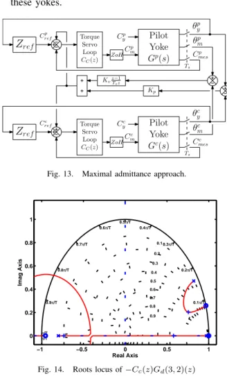
The maximal admittance solution is depicted in Fig.13 and involves:

• an inner torque servo-loop through the controller

Cc(z) = 0.17z

2_−1.932z+1

(z−1)(z+0.8), that is: an integral action

with a notch filter to damp the flexible mode. The roots locus of the inner loop is depicted in Fig.14,

• an outer feedback from the angular position of the

yoke θ_y to the torque input reference C_ref through

the impedance reference model Z_ref(z) (that is: the

continuous to discrete time conversion of the regularized

impedance model Z_ref(s) (in order to be a proper

transfer),

• a proportional derivative control (through gainsK_pand

Kv) of the two yokes relative position in order to couple

these yokes. Pilot Yoke Gp_(s) θp y Cp mes θp m ZoH Torque Servo Loop CC(z) Cp y Zref Cp ref Cp m Ts Pilot Yoke Gc_(s) θc y Cc mes θc m ZoH Torque Servo Loop CC(z) Cc y Zref Cc ref Cc m Ts Kvz−1Tsz Kp

Fig. 13. Maximal admittance approach.

−1 −0.5 0 0.5 1 0 0.2 0.4 0.6 0.8 1 0.9 0.8 0.7 0.6 0.5 0.4 0.3 0.2 0.1 π/T π/T 0.9π/T 0.8π/T 0.7π/T 0.6π/T 0.5π/T 0.4π/T 0.3π/T 0.2π/T 0.1π/T Real Axis Imag Axis

Fig. 14. Roots locus of −Cc(z)G_d(3, 2)(z)

This solution is called maximal admittance solution (or minimal impedance solution) because the torque servo-loop is tuned very stiff in such way that if the torque input

reference is set to0 (i.e. Z_ref(s) = 0), the actuator works

with the pilot torque C_y (to cancel the measured torque)

then the yoke seems to be completely free and ”light” i.e. the admittance is very great. The response of the admittance once the torque servo-loop is closed is depicted in Fig.7 (red plot).