Robust impedance active control of flight control devices
Texte intégral
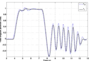
Figure

Documents relatifs
The objective of this paper is design a New Robust Control for Doubly fed Induction Machine based on Type-2 Fuzzy Logic Controller , The term fuzzy Presented by a controller
The main contribution of this paper is to optimize in a single step the control surfaces span, the control allocation module, and flight control laws, in order to guarantee
This paper focuses on the design of a centralized control system robust to asymmetrical downlink packet losses in a mixed MDV/CACC scenario. The key contributions are as fol- lows:
The phase slope of the FRF has been used in the design of fractional order PD/PI controller based on an auto-tuning method that requires knowledge of the process modulus, phase
On the other hand, recall from linear systems theory, that quite basic tools such as the Bode diagram permit to design the cut-off frequency of a linear controller in order to
The remainder of this paper is structured as follows: Section 2 shows our method for over-bounding Hermitian terms via Elimination lemma; Section 3 shows the proposed design method
The main contribution of this paper is the design of a robust finite time convergent controller based on geometric homogeneity and sliding mode control which can be easily applied
HIGH ORDER SLIDING MODE CONTROLLER The use of assumptions for the model design implies that, if a high accuracy in position control is the objective, a robust control law with
