Modes dégradés résultant de l'utilisation multi constellation du GNSS

(1)

ccc

T

H

È

S

E

En vue de l'obtention du

D

O

C

T

O

R

A

T

D

E

L

’

U

N

I

V

E

R

S

I

T

É

D

E

T

O

U

L

O

U

S

E

Délivré par l’Institut National Polytechnique de Toulouse Discipline ou spécialité : télécommunications - SIAO

Ecole doctorale : Mathématiques Informatique Télécommunications de Toulouse

JURY

Pr Francis Castanié (Président) Pr Igor Nikiforov (Rapporteur) Pr Bernd Eissfeller (Rapporteur) Dr Christophe Macabiau (Directeur)

Dr Benoît Roturier (Examinateur)

Présentée et soutenue par Christophe OUZEAU Le 08/04/2010

Titre : Modes dégradés résultant de l’utilisation multi constellation du GNSS Title : Degraded Modes Resulting From the Multi Constellation Use of GNSS

(2)

(3)

Résumé

Actuellement, on constate dans le domaine de la navigation, un besoin croissant de localisation par satellites. Après une course à l’amélioration de la précision (maintenant proche de quelques centimètres grâce à des techniques de lever d’ambiguïté sur des mesures de phase), la relève du nouveau défi de l’amélioration de l’intégrité du GNSS (GPS, Galileo) est à présent engagée. L’intégrité représente le degré de confiance que l’on peut placer dans l’exactitude des informations fournies par le système, ainsi que la capacité à avertir l’utilisateur d’un dysfonctionnement du GNSS dans un délai raisonnable.

Le concept d’intégrité du GNSS multi-constellation nécessite une coordination au niveau de l’architecture des futurs récepteurs combinés (GPS-Galileo). Le fonctionnement d’un tel récepteur dans le cas de passage du système multi-constellation en mode dégradé est un problème très important pour l’intégrité de navigation.

Cette thèse se focalise sur les problèmes liés à la navigation aéronautique multi-constellation et multi-système GNSS. En particulier, les conditions de fourniture de solution de navigation intègre sont évaluées durant la phase d’approche APV I (avec guidage vertical). En disposant du GPS existant, du système Galileo et d’un système complémentaire géostationnaire (SBAS), dont les satellites émettent sur des fréquences aéronautiques en bande ARNS, la question fondamentale est comment tirer tous les bénéfices d’un tel système multi-constellation pour un récepteur embarqué à bord d’un avion civil. En particulier, la question du maintien du niveau de performance durant cette phase de vol APV, en termes de précision, continuité, intégrité et disponibilité, lorsque l’une des composantes du système est dégradée ou perdu, doit être résolue.

L’objectif de ce travail de thèse est donc d’étudier la capacité d’un récepteur combiné avionique d’effectuer la tâche de reconfiguration de l’algorithme de traitement après l’apparition de pannes ou d’interférences dans une partie du système GNSS multi-constellation et d’émettre un signal d’alarme dans le cas où les performances de la partie du système non contaminée ne sont pas suffisantes pour continuer l’opération en cours en respectant les exigences de l’aviation civile. Egalement, l’objectif de ce travail est d’étudier les méthodes associées à l’exécution de cette reconfiguration pour garantir l’utilisation de la partie du système GNSS multi-constellation non contaminée dans les meilleures conditions. Cette étude a donc un intérêt pour les constructeurs des futurs récepteurs avioniques multi-constellation.

(4)

Abstract

The International Civil Aviation Organization (ICAO) has defined the concept of Global Navigation Satellite System (GNSS), which corresponds to the set of systems allowing to perform satellite-based navigation while fulfilling ICAO requirements.

The US Global Positioning Sysem (GPS) is a satellite-based navigation system which constitutes one of the components of the GNSS. Currently, this system broadcasts a civil signal, called L1 C/A, within an Aeronautical Radio Navigation Services (ARNS) band. The GPS is being modernized and will broadcast two new civil signals: L2C (not in an ARNS band) and L5 in another ARNS band.

Galileo is the European counterpart of GPS. It will broadcast three signals in an ARNS band: Galileo E1 OS (Open Service) will be transmitted in the GPS L1 frequency band and Galileo E5a and E5b will be broadcasted in the same 960-1215 MHz ARNS band than that of GPS L5.

GPS L5 and Galileo E1, E5a, E5b components are expected to provide operational benefits for civil aviation use. However, civil aviation requirements are very stringent and up to now, the bare systems alone cannot be used as a means of navigation. For instance, the GPS standalone does not implement sufficient integrity monitoring.

Therefore, in order to ensure the levels of performance required by civil aviation in terms of accuracy, integrity, continuity of service and availability, ICAO standards define different systems/algorithms to augment the basic constellations. GPS, Galileo and the augmentation systems could be combined to comply with the ICAO requirements and complete the lack of GPS or Galileo standalone performance.

In order to take benefits of new GNSS signals, and to provide the service level required by the ICAO, the architecture of future combined GNSS receivers must be standardized. The European Organization for Civil Aviation Equipment (EUROCAE) Working Group 62, which is in charge of Galileo standardization for civil aviation in Europe, proposes new combined receivers architectures, in coordination with the Radio Technical Commission for Aeronautics (RTCA).

The main objective of this thesis is to contribute to the efforts made by the WG 62 by providing inputs necessary to build future receivers architecture to take benefits of GPS, Galileo and augmentation systems. In this report, we propose some key elements of the combined receivers’ architecture to comply with approach phases of flight requirements.

In case of perturbation preventing one of the needed GNSS components to meet a phase of flight required performance, it is necessary to be able to switch to another available component in order to try to maintain if possible the level of performance in terms of continuity, integrity, availability and accuracy. That is why future combined receivers must be capable of detecting the impact of perturbations that may lead to the loss of one GNSS component, in order to be able to initiate a switch. These perturbations are mainly atmospheric disturbances, interferences and multipath. In this thesis we focus on the particular cases of interferences and ionosphere perturbations.

(5)

The interferences are among the most feared events in civil aviation use of GNSS. Detection, estimation and removal of the effect of interference on GNSS signals remain open issues and may affect pseudorange measurements accuracy, as well as integrity, continuity and availability of these measurements. In literature, many different interference detection algorithms have been proposed, at the receiver antenna level, at the front-end level. Detection within tracking loops is not widely studied to our knowledge. That is why, in this thesis, we address the problem of interference detection at the correlators outputs. The particular case of CW interferences detection on the GPS L1 C/A and Galileo E1 OS signals processing is proposed.

Nominal dual frequency measurements provide a good estimation of ionospheric delay. In addition, the combination of GPS or GALILEO navigation signals processing at the receiver level is expected to provide important improvements for civil aviation. It could, potentially with augmentations, provide better accuracy and availability of ionospheric correction measurements. Indeed, GPS users will be able to combine GPS L1 and L5 frequencies, and future GALILEO E1 and E5 signals will bring their contribution. However, if affected by a Radio Frequency Interference, a receiver can lose one or more frequencies leading to the use of only one frequency to estimate the ionospheric code delay.

Therefore, it is felt by the authors as an important task to investigate techniques aimed at sustaining multi-frequency performance when a multi constellation receiver installed in an aircraft is suddenly affected by radiofrequency interference, during critical phases of flight. This problem is identified for instance in [NATS, 2003]. Consequently, in this thesis, we investigate techniques to maintain dual frequency performances when a frequency is lost (L1 C/A or E1 OS for instance) after an interference occurrence.

(6)

Remerciements / Acknowledgments

Je tiens tout d’abord à remercier mon directeur de thèse, Christophe Macabiau. Tu m’as permis de commencer cette thèse dans de bonnes conditions. Tes conseils précieux m’ont permis d’améliorer considérablement mon travail. De plus, je te remercie pour avoir relu à plusieurs reprises ce rapport. Merci aussi pour tes qualités humaines et tes rires bruyants.

Merci à Benoît d’avoir cru en ce travail et m’avoir permis de mener à bout ces travaux de recherche.

Merci à Frédéric Bastide pour la qualité de son encadrement et ses conseils avisés lors des premiers mois de cette thèse.

I thank all the EUROCAE members for their remarks about this thesis. I was really pleased to work with you. I’d like to thanks in particular, Benoît, Mikael, Laurent and Eric. It was really a pleasure to work with you!

Merci au Professeur Igor Nikiforov pour avoir accepté d’être rapporteur de cette thèse et merci pour tous ses conseils.

I would like also to thank Pr Bernd Eissfeller for being my reviewer and for its remarks and advices during my PhD defense.

Merci à Francis Castanié pour avoir été mon président de jury de thèse, pour sa sympathie, mais aussi pour toutes les discussions intéressantes que nous avons eues tout au long des mon séjour au TéSA.

Je remercie tous mes anciens collègues du LTST dans l’ordre alphabétique : Axel, Damien, Damien, Emilie, Hanaa, Anais, Mathieu, Na, Olivier, Anne-Christine, Paul, Philippe et Gaël. Merci à vous tous pour ces excellentes conditions de travail. Ce fut un plaisir de travailler en votre compagnie.

Je tiens à remercier Hanaa, Na et Cyril pour leurs relectures de ce rapport et leurs conseils avisés.

J’ai été très heureux de pouvoir travailler en compagnie de nombreux collègues d’une grande sympathie et d’une grande générosité à l’ENAC. Je ne peux malheureusement tous vous citer tant vous êtes nombreux ! Merci à Coco et Cathy pour leur soutien administratif mais aussi humain.

Un grand merci aussi à tous les collègues du TéSA. Je pense en particulier à Marie-Jo et Sarah, dont la bonne humeur a ensoleillé chaque matin de mes passages au TéSA. Merci aussi les filles pour la préparation de mes nombreuses missions parfois un peu compliquées !

I really thank Chris Hegarty for giving me advices about ionospheric code delay estimations and for our pleasant discussions about my thesis and some professional points.

(7)

Sommaire / Outline

RESUME III

ABSTRACT IV

REMERCIEMENTS / ACKNOWLEDGMENTS VI

SOMMAIRE / OUTLINE VII

LIST OF FIGURES XIII

LIST OF TABLES XV

GLOSSARY XVI

1. INTRODUCTION 2

1.1. BACKGROUND AND MOTIVATIONS 2

1.2. THESIS OUTLINE 3

1.3. THESIS ORIGINAL CONTRIBUTIONS 5

RESUME 4

2. GNSS APPLIED TO CIVIL AVIATION OPERATIONS 5

2.1. INTRODUCTION 5

2.2. CIVIL AVIATION APPLICATION 5

2.2.1. INTRODUCTION 5

2.2.2. CIVIL AVIATION OPERATIONS 5

2.2.2.1. Phases of flight 5

2.2.2.1.1. Non-precision approach (NPA) 5 2.2.2.1.2. Approach and landing operations with vertical guidance (APV) 6 2.2.2.1.3. CAT-I, CAT-II, CAT-III precision approach 6 2.2.2.1.4. Missed Approach (MA) 6

2.2.2.2. ICAO requirements 7

2.2.2.3. Accuracy 7

2.2.2.4. Integrity 7

2.2.2.5. Availability 9

2.2.2.6. Continuity of service 9 2.2.2.7. ICAO performance requirements for each phase of flight 9

2.3. DEFINITION AND DESCRIPTION OF GNSS 10

2.3.1. GNSS PRINCIPLE AND MEASUREMENTS 10

2.3.2. GNSS MEASUREMENTS FOR CIVIL AVIATION USE 11

2.3.2.1. Smoothing process and civil aviation requirement 12 2.3.2.2. Least squares position solution 13

2.3.3. GNSS COMPONENTS 15

2.3.3.1. GPS 15

(8)

2.3.3.3. Augmentation systems 16 2.3.3.3.1. Aircraft Based Augmentation System 16 2.3.3.3.1.1. Protection levels calculation 17 2.3.3.3.2. Satellite Based Augmentation System 18 2.3.3.3.2.1. Protection levels calculation 19 2.3.3.3.3. Ground Based Augmentation System 21

2.3.4. GNSS SERVICES 21

2.3.4.1. Galileo services [ESA, 2004] 21 2.3.4.1.1. Safety Of Life (SoL) 21

2.3.4.1.2. Open Service (OS) 21

2.3.4.1.3. Public Regulated Service (PRS) 21 2.3.4.1.4. Commercial Service (CS) 22 2.3.4.1.5. Search And Rescue service (SAR) 22

2.3.4.2. Conclusion 22 2.3.5. SIGNALS CHARACTERISTICS 22 2.3.5.1. GPS L1 signals 23 2.3.5.2. GPS L5 23 2.3.5.3. Galileo E1 24 2.3.5.4. Galileo E5a/E5b 25 2.3.5.5. Conclusion 26 2.3.6. SIGNALS RECEPTION 26 2.3.7. RF SIGNAL CONDITIONING 26 2.3.7.1. Antenna 27 2.3.7.2. Preamplification 27 2.3.7.3. Reference oscillator 27 2.3.7.4. Frequency synthesizer 27 2.3.7.5. Down conversion and filtering 28 2.3.7.6. Sampling and quantization 28 2.3.7.7. Digital signal processing 28

2.3.7.7.1. Acquisition 29

2.3.7.7.2. Acquisition to tracking transition 30

2.3.7.7.3. Tracking 30

2.3.7.7.4. Correlation 31

2.3.7.7.5. Discriminators 33

2.3.7.7.6. Loop filters 34

2.3.7.8. Conclusions 35

2.4. PERTURBATIONS AFFECTING GNSS SIGNALS 35

2.4.2. IONOSPHERE 35

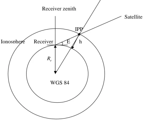
2.4.2.1. THIN SHELL MODEL 40

2.4.3. TROPOSPHERE 41

2.4.4. MULTIPATH 41

2.4.5. INTERFERENCES 42

2.4.6. SATELLITE CLOCK ERROR 43

2.4.7. RECEIVER DYNAMICS 43

2.5. CONCLUSIONS 44

RESUME 47

3. COMBINED USE OF GNSS COMPONENTS AND RECEIVER ARCHITECTURE 48

3.1. DEFINITION OF MODES OF OPERATION 48

(9)

3.1.2. ALTERNATE MODE 48

3.1.3. DEGRADED MODE 48

3.1.4. CONCLUSION 49

3.2. GNSS COMBINATIONS IDENTIFIED BY THE EUROCAEWG62 49

3.3. GLOBAL CIVIL AVIATION COMBINED RECEIVERS ARCHITECTURE 51

3.3.2. GLOBAL RECEIVER SWITCHING ARCHITECTURE 52

3.4. THE NAVIGATION FUNCTION 53

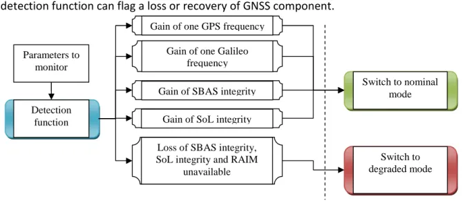
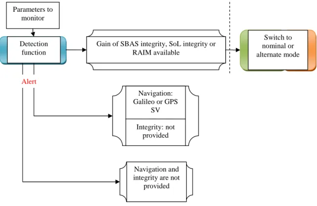
3.5. THE DETECTION FUNCTION 53

3.5.1. DETECTION ALGORITHMS AND CIVIL AVIATION REQUIREMENTS 53

3.5.3. DETECTION FUNCTION AND PERFORMANCE LEVELS 54

3.6. CONCLUSION 55

RESUME 58

4. DETECTION OF DEGRADATIONS AND RECONFIGURATION OF THE NAVIGATOR

IN CASE OF DEGRADED MODE 59

4.2. STRATEGY FOR EACH MODE OF OPERATION 59

4.2.1. NOMINAL MODE STRATEGY FOR EN ROUTE DOWN TO NPA 59

4.2.2. ALTERNATE MODE STRATEGY FOR EN ROUTE DOWN TO NPA 61

4.2.3. DEGRADED MODE STRATEGY FOR EN ROUTE DOWN TO NPA 62

4.2.4. NOMINAL MODE STRATEGY FOR APVI 63

4.2.5. ALTERNATE MODE STRATEGY FOR APVI 64

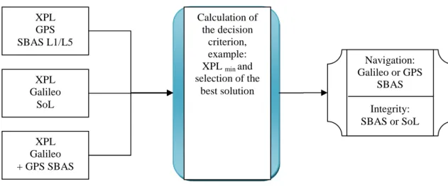
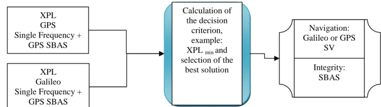
4.2.6. DEGRADED MODE STRATEGY FOR APVI 65

4.3. NAVIGATOR RECONFIGURATION IN CASE OF DEGRADED MODE 66

4.4. CONCLUSION 67

RESUME 71

5. PERFORMANCE OF MULTI CORRELATORS GNSS INTERFERENCE DETECTION

AND REPAIR ALGORITHMS 72

5.2. REVIEW OF EXISTING INTERFERENCE DETECTION TECHNIQUES 72

5.2.1. DETECTION TECHNIQUES AT THE RECEIVER FRONT END LEVEL 73

5.2.1.1. Chi-square test at the ADC Level 73 5.2.1.2. Temporal blanker and FDIS 73

5.2.2. INTERFERENCE DETECTION WITHIN THE TRACKING LOOPS 73

5.2.2.1. Computation of the Signal to Noise Ratio (SNR) 73 5.2.2.2. Detection at the correlators outputs 73

5.3. GNSS SIGNALS STUDIED 74

5.3.1. BUDGET OF SIGNALS POWER 76

5.4. IMPACT OF CW INTERFERENCES ON SIGNALS PROCESSING 77

5.4.1. CODE SPECTRUM LINES CORRELATED WITH INTERFERENCES 77

5.4.1.1. Identified worst case code spectrum lines 79 5.4.1.2. Position of the interference in the code spectrum 79

(10)

5.4.3. OBSERVED INFLUENCE ON TRACKING LOOPS 84

5.5. ELABORATION OF THE INTERFERENCES DETECTION TECHNIQUES 86

5.5.1. MULTI CORRELATORS DETECTION ALGORITHMS 86

5.5.2. PROPOSED DETECTION TECHNIQUES AT THE CORRELATORS OUTPUTS 87

5.5.2.1. Computation of the FFT of the correlators outputs 87 5.5.2.2. Multichannel Autoregressive model of correlator outputs 88

5.6. DETECTION ALGORITHMS PERFORMANCES EVALUATION PROCESS 90

5.7. SIMULATIONS ASSUMPTIONS 90

5.7.1. SIMULATION OF ACTUAL AIRCRAFT APPROACH CONDITIONS 90

5.7.1.1. Aircraft dynamics 91

5.7.1.2. Doppler shift rate between aircraft, satellites in view and interference source 91

5.7.1.3. Multipath 94

5.7.2. GENERATED SIGNALS POWER 95

5.7.3. RECEIVER SETTINGS 95

5.7.3.1. Tracking loops 95

5.7.3.2. Multiple correlators settings 95

5.8. SIMULATION RESULTS 96

5.8.1. OBTAINED PMD AND UNDETECTED ERRORS INDUCED IN PSEUDORANGES MEASUREMENTS BY USING THE FIRST

FFT-BASED ALGORITHM 96

5.8.2. OBTAINED PMD BY USING THE SECOND AR-BASED ALGORITHM 99

5.9. DISCUSSION ABOUT THE OBTAINED RESULTS 99

5.10. CONCLUSION AND FUTURE WORKS ON INTERFERENCE DETECTION 100

5.10.1. DISCUSSION ABOUT THE PROPOSED ALGORITHMS AND CIVIL AVIATION REQUIREMENTS 101

5.11. USE OF A MODEL TO CHARACTERIZE EACH INTERFERENCE 101

5.12. CONCLUSION 103

5.12.1. SCENARII WITH REGARD TO THE COMBINED RECEIVER ARCHITECTURE 104

RESUME 108

6. IONOSPHERIC CODE DELAY ESTIMATION IN CASE OF SINGLE FREQUENCY

DEGRADED MODE 109

6.1. INTRODUCTION 109

6.2. DUAL FREQUENCY IONOSPHERIC CODE DELAY ESTIMATION 110

6.2.1. APPLICATION TO FUTURE GNSS SIGNALS 111

6.3. ESTIMATION OF THE IONOSPHERIC CODE DELAY THANKS TO ESTIMATION MODELS 113

6.3.1. GPSKLOBUCHAR MODEL 113

6.3.2. GALILEO NEQUICK MODEL 114

6.3.3. ADVANTAGES AND DRAWBACKS OF THE ESTIMATION MODELS 115

6.4. SINGLE FREQUENCY CODE MINUS CARRIER DIVERGENCE TECHNIQUE TO ESTIMATE

IONOSPHERIC CODE DELAY 117

6.4.1. METHOD 117

6.4.2. ACCURACY OF THE METHOD 117

6.4.3. CYCLE SLIPS 118

6.4.3.1. Cycle slip occurrence rate 119 6.4.3.2. Cycle slip and integrity for APV 122 6.4.3.3. Cycle slip detection methods 123 6.4.3.3.1. Cycle slip detection using Doppler measurements 123 6.4.3.4. Smallest detectable cycle slip 124 6.4.3.4.1. Measurements simulator 124

(11)

6.4.3.4.1.2. Clock bias 125

6.4.3.4.1.3. Multipath 126

6.4.3.4.1.4. Troposphere 126

6.4.3.4.1.5. Ionosphere 126

6.4.3.4.1.6. Noise 126

6.4.3.4.2. Estimation of the smallest detectable cycle slip with the proposed detection algorithm 127 6.4.3.4.3. Cycle slip detection availability calculation 130 6.4.3.4.4. Maps of availability of cycle slip detection algorithm for GPS and Galileo constellations

133

6.5. IONOSPHERIC DELAY ESTIMATION USING KALMAN FILTER ON CMC OBSERVABLES 135

6.5.1. FILTER SETTINGS AND CHARACTERISTICS 135

6.5.3. KALMAN FILTER ESTIMATION IN SINGLE FREQUENCY MODE 142

6.6. CONCLUSION AND FUTURE WORKS 144

7. CONCLUSION AND FUTURE WORKS 147

7.1. GLOBAL GOALS AND COMBINED RECEIVER ARCHITECTURE 147

7.2. INTERFERENCE THREAT 147

7.2.1. INTERFERENCE DETECTION FOR INTEGRITY AND CONTINUITY 147

7.2.2. INTERFERENCE REMOVAL FOR ACCURACY 148

7.2.3. RECOMMENDATIONS AND FUTURE WORKS ON INTERFERENCE THREAT 149

7.3. SINGLE FREQUENCY DEGRADED MODE 149

7.3.1. IONOSPHERIC CODE DELAY ESTIMATION FOR ACCURACY 149

7.3.2. CYCLE SLIP DETECTION FOR INTEGRITY 149

7.3.3. AVAILABILITY OF THE ALGORITHM 149

7.3.4. RECOMMENDATIONS AND FUTURE WORKS FOR SINGLE FREQUENCY IONOSPHERIC DELAY ESTIMATION 150

7.4. RECOMMENDATIONS AND FUTURE WORKS 150

REFERENCES - 153 -

AUTHOR PUBLICATIONS PRESENTED FOR THIS PHD THESIS - 162 -

APPENDIX A: MATHEMATICAL MODELS 164

APPENDIX A.1:ARMA MODEL 164

APPENDIX A.2:MULTICHANNEL AUTOREGRESSIVE MODEL 166

APPENDIX A.3:PRONY MODEL 171

APPENDIX A.4:PROBABILITY OF INTERFERENCE OCCURRENCE 174

APPENDIX B: AIRCRAFT ENVIRONMENT 177

APPENDIX B.1:MODEL OF AIRCRAFT DYNAMICS 177

APPENDIX B.2:MULTIPATH GENERATION 180

APPENDIX B.3:DUAL FREQUENCY IONOSPHERIC ERROR ESTIMATION 185

APPENDIX C: RECEIVERS AND SIGNALS CHARACTERISTICS 186

APPENDIX C.1:RECEIVERS CLASSES 186

(12)

(13)

List of figures

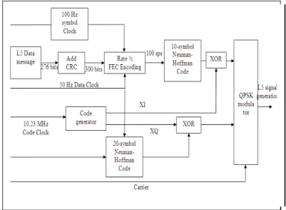
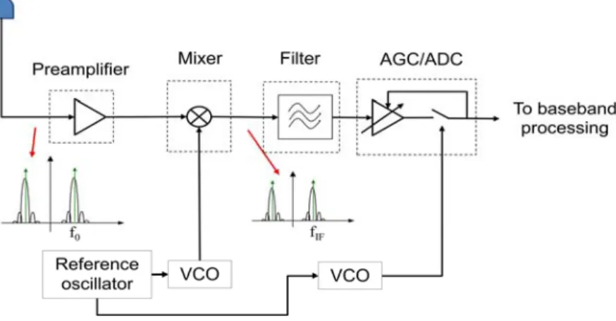
Figure 1: EGNOS theoretical coverage [ESA, 2004]. ____________________________________________ 19 Figure 2: Galileo and GPS frequency plan, [GSA, 2008] _________________________________________ 23 Figure 3: GPS L1 C/A generation____________________________________________________________ 23 Figure 4: GPS L5 generation _______________________________________________________________ 24 Figure 5: Galileo E1 (B+C) generation _______________________________________________________ 25 Figure 6: Galileo E5a generation ____________________________________________________________ 26 Figure 7: Galileo E5b generation ____________________________________________________________ 26 Figure 8: RF signal conditioning until digitalization, VCO stands for Voltage Control Oscillator __________ 27 Figure 9: Acquisition process _______________________________________________________________ 29 Figure 10: Tracking process ________________________________________________________________ 31 Figure 11: Correlation process______________________________________________________________ 32 Figure 12: Costas discriminator _____________________________________________________________ 34 Figure 13: Arctan discriminator _____________________________________________________________ 34 Figure 14: Time of arrival of code and carrier phase of each signal _________________________________ 38 Figure 15: Geometrical parameters for obliquity calculation ______________________________________ 40 Figure 16: Switching between modes of operation _______________________________________________ 53 Figure 17: Links between accuracy, integrity, continuity and availability of GNSS components [Chatre, 2003] 55 Figure 18: Navigation function for en-route down to NPA operations with nominal mode ________________ 59 Figure 19: Detection function for en-route down to NPA operations with nominal mode _________________ 61 Figure 20: Navigation function for en-route down to NPA operations with alternate mode _______________ 62 Figure 21: Detection function for en-route down to NPA operations with alternate mode ________________ 62 Figure 22: Navigation function for en-route down to NPA operations with degraded mode _______________ 63 Figure 23: Detection function for en-route down to NPA operations with alternate mode ________________ 63 Figure 24: Navigation function for APV I operation with nominal mode ______________________________ 64 Figure 25: Detection functions for APV I operation with nominal mode ______________________________ 64 Figure 26: Navigation function for APV I operation with alternate mode _____________________________ 65 Figure 27: Detection function for APV I operation with alternate mode ______________________________ 65 Figure 28: Navigation function for APV I operations with degraded mode ____________________________ 65 Figure 29: Detection function for APV I operations with degraded mode _____________________________ 66 Figure 30: E1 PSD in an already crowded L1 frequency band _____________________________________ 74 Figure 31: BPSK waveform and corresponding autocorrelation function _____________________________ 75 Figure 32: BOC (fs,fc) waveform and corresponding autocorrelation function _________________________ 75 Figure 33: BPSK, BOC and CBOC correlation function __________________________________________ 76 Figure 34: GPS L1 C/A code spectrum ________________________________________________________ 78 Figure 35: Galileo E1OS code spectrum ______________________________________________________ 78 Figure 37 : Simulated correlators outputs on the I GPS L1 C/A channel affected by CW interference. ______ 83 Figure 38 : C/N0 estimated at the correlator output without CW, and with generated interfering CW, 200 seconds after the beginning of the simulation. __________________________________________________ 84 Figure 39 : Phase tracking error with a 10 Hz PLL bandwidth and a dot product discriminator on the left side and raw code tracking error using a 1Hz DLL bandwidth, with CW after 200 seconds simulation, the Doppler shift rate equals 2 Hz/s. ____________________________________________________________________ 84 Figure 40 : Impact of the interference power on the code tracking loop accuracy, with the same tracking settings, fighting GPS L1 C/A PRN 6 worst code spectrum line. ____________________________________ 86 Figure 41 : Normalized GPS L1 C/A correlators outputs. _________________________________________ 87 Figure 42 : Time variations of correlators for GPS L1 C/A signal affected by a – 155 dBW CW interference on the PRN 6 worst case line (227 kHz), without Doppler shift. The variations at the top corresponding to a correlator near the peak (0.32 chip away), the bottom correlator variations corresponds to a correlator located 1.6 chip away from the peak. _______________________________________________________________ 89 Figure 36: Satellite-aircraft-jammer configuration ______________________________________________ 91 Figure 43 : Amplitude of maximum tracking error as a function of interference power resulting from non-detected CW on the GPS ___________________________________________________________________ 97 Figure 44 : Amplitude of maximum tracking errors as a function of interference power resulting from non-detected CW on the GPS L1 C/A code, PRN 2, the useful signal power is -158.5 dBW. __________________ 97 Figure 45 : Amplitude of maximum tracking errors as a function of interference power resulting from non-detected CW on the GPS L1 C/A code, PRN 10, the power of the useful signal is -158.5 dBW._____________ 98 Figure 46 : Amplitude of maximum tracking errors as a function of interference power resulting from non-detected CW on the Galileo E1 code, PRN 38, the power of the useful signal is -160 dBW. _______________ 98

(14)

Figure 47 : Obtained missed detection classified by resulting raw tracking errors for GPS L1 C/A PRN 6 highest code spectrum line impacted by one -155 dBW CW interference. _____________________________ 99 Figure 48 : Estimation of a -155 dBW CW frequency impacting GPS L1 C/A PRN 6 (227 kHz) using a third order Prony model on 68 correlators outputs. _________________________________________________ 102 Figure 49 : Raw code tracking error with and without one -155 dBW CW interference estimation and correction, the impacted code spectrum line is the PRN 6 (227 KHz) of the L1 C/A signal.________________________ 103 Figure 50: Interference detection function based on correlators outputs monitoring ___________________ 105 Figure 51: Klobuchar function: evolution of single atmospheric layer located at 350 km high ____________ 113 Figure 52: Variations of the electronic density estimated with the NeQuick model as a function of the altitude at the zenith of Toulouse (position: latitude: 43.56475924°N, longitude: 1.48171036°E, altitude: 203.845 m). _ 115 Figure 53: L1slant ionospheric delay estimated thanks to the CMC technique, for a receiver located at ENAC, Toulouse, France, on 14/03/2006. A cycle slip occurs for a low elevation angle of about 20 degrees, which may correspond to a multipath. ________________________________________________________________ 119 Figure 54: Cycle slip occurrence probability using different phase tracking loops for maximum normal

dynamics, calculated for 1 second, with a 20 ms integration time for GPS L1 C/A, Coh stands for coherent and corresponds to a classical PLL. ____________________________________________________________ 120 Figure 55: Cycle slip occurrence probability using different phase tracking loops for maximum normal dynamics on the left side and abnormal aircraft dynamics on the right side, calculated for 1 second, with a 4 ms

integration time for GPS L1 C/A, Coh stands for coherent and corresponds to a classical PLL. __________ 121 Figure 56: Probability of False Alarm obtained through simulations as a function of detection thresholds for both maximum normal and abnormal manoeuvres (step 1). _______________________________________ 128 Figure 57: Probability of Missed Detection of the cycle slip detection algorithm with regards to integrity requirements for APV, obtained by simulating different cycle slip amplitudes (bias), the PMD are recorded for

each cycle slip amplitude and compared to theoretical PMD values for both normal and abnormal aircraft

manoeuvres (step 2). _____________________________________________________________________ 129 Figure 58: Computed position error for all satellites in view. _____________________________________ 132 Figure 59: Availability of proposed cycle slip detection algorithm over Europe considering GPS constellation only and normal aircraft dynamics, for APV 1 alert limits. _______________________________________ 134 Figure 60: Availability of proposed cycle slip detection algorithm over Europe considering Galileo constellation only and normal aircraft dynamics for APV 1 alert limits. ________________________________________ 134 Figure 61: Obliquity factor as a function of the elevation in degrees________________________________ 137 Figure 62: Aircraft path, data collected from Airbus campaign, zoom on the Blagnac Airport (Toulouse, France), ©Airbus. _______________________________________________________________________ 139 Figure 63: Aircraft path, data collected from Airbus campaign around Blagnac Airport (Toulouse, France), ©Airbus. ______________________________________________________________________________ 140 Figure 64: Eurocontrol Pegasus Software ____________________________________________________ 140 Figure 65: Number of satellites tracked as a function of time samples ______________________________ 141 Figure 66: GPS L1 C/A code measurements for all tracked satellites over the entire file ________________ 141 Figure 67: GPS L2 code measurements for all tracked satellites over the entire file ____________________ 141 Figure 68: GPS L1 C/A carrier phase measurements for all tracked satellites ________________________ 142 Figure 69: Ionospheric code delay estimated thanks to dual frequency measurements during the aircraft flight, the presented results are weighted by the obliquity factors. _______________________________________ 142 Figure 70: Ionospheric code delay estimated by the Kalman filter (in red) versus mean dual frequency

estimation over all the acquired satellites (in green). ____________________________________________ 143 Figure 71: Innovation plotted for the SV 7. ___________________________________________________ 144 Figure 72 : Dynamics generation according to the acceleration and jerk values (divided by the speed of light) _____________________________________________________________________________________ 178 Figure 73: Multipath aircraft fuselage _______________________________________________________ 180 Figure 74: Multipath ground reflection ______________________________________________________ 181 Figure 75 : Multipath generation on an A 340 over 500-seconds simulation during landing, taking into account fuselage and ground reflections ____________________________________________________________ 184 Figure 76: Class Beta Architecture [EUROCAE, 2007] _________________________________________ 187 Figure 77: Class Delta Architecture [EUROCAE, 2007] _________________________________________ 187 Figure 78: Receivers functional classes as defined in [RTCA, 2006]. _______________________________ 188

(15)

List of tables

Table 1: GNSS SIS requirements from [ICAO, 2006]. ____________________________________________ 10 Table 2: Normal and Abnormal aircraft dynamics, [EUROCAE, 2007]. ______________________________ 43 Table 3: Identified nominal, alternate and degraded modes for en route to NPA and APV I phases of flight [EUROCAE, 2008]. ______________________________________________________________________ 50 Table 4: Specified received power and carrier to noise ratios required at tracking level, [EUROCAE, 2007]. 77 Table 5 : Carrier to noise ratios for GPS and Galileo signals used during simulations. __________________ 77 Table 7 : Simulator tracking characteristics. ___________________________________________________ 84 Table 6 : Doppler shift rate values obtained through simulations. ___________________________________ 94 Table 5 : Carrier to noise ratios for GPS and Galileo signals used during simulations. __________________ 95 Table 7 : Simulator tracking characteristics. ___________________________________________________ 95 Table 8: Raw and smoothed code tracking error with and without interference removal at the correlator output level, over 80 seconds (4000 samples). _______________________________________________________ 103 Table 9: Comparison between Klobuchar and NeQuick models [Belabbas, 2005] and [NATS, 2003]. _____ 116 Table 10: Comparison between dual and single frequency ionosphere estimation standard deviations at Gatwick and Swanwick (UK), [NATS, 2003]. _________________________________________________________ 117 Table 11: Probability of cycle slip occurrence for a Costas PLL, with 10 Hz bandwidth and coherent integration time TI.________________________________________________________________________________ 122

Table 12: Oscillators characteristics, [Winkel, 2003]. ___________________________________________ 125 Table 13: Mean and STD of dual and single frequency estimations of mean ionospheric code delay over all the tracked satellites. _______________________________________________________________________ 143 Table 14: States of the ground fading Markov model ___________________________________________ 183 Table 15: Combinations to be standardized [EUROCAE, 2007]. __________________________________ 187 Table 16 : Worst line characteristics for each PRN for GPS C/A code. ______________________________ 189 Table 17: Worst line characteristics for each PRN for GALILEO E1 code. ___________________________ 190

(16)

Glossary

AAIM Aircraft-based Autonomous Integrity Monitoring

ABAS Aircraft Based Augmentation System

AIC Aeronautical Information Circular

AIP Aeronautical Information Publication

AIRAC Aeronautical Information Regulation And Control

AMC Acceptable Means of Compliance

ANP Actual Navigation Performance

APV ARNS

Approach with Vertical Guidance Aeronautical Radio Navigation Services

ARINC Aeronautical Radio Incorporated

ATC Air Traffic Control

BER Bit Error Rate

CDI Course Deviation Indicator

CDU Cockpit Display Unit

CONUS CONtinental United States

DAC Direction de l’Aviation Civile

DLL Delay Lock Loop

DTK Desired Track

DER Departure End of the Runway

DME Distance Measuring Equipment

EASA European Aviation Safety Agency

ECAC European Civil Aviation Conference

EGNOS European Global Navigation Overlay Service

EPE Estimated Position Error

EPU Estimated Position Uncertainty

ETA Estimated Time of Arrival

EUROCAE European Organization for Civil Aviation Equipment

FAF Final Approach Fix

FAS Final Approach Segment

FDE Fault Detection and Exclusion

FFS Full Flight Simulator

FMC Flight Management Computer

FMS Flight Management System

FNPT Flight Navigation and Procedure Trainer

FTD Flight Training Device

FTE Flight Technical Error

GBAS Ground Based Augmentation System

GLONASS GLObal NAvigation Satellite System

GNSS Global Navigation Satellite System (OACI terminology)

GPS Global Positioning System

GGTO GPS Galileo Time Offset

IAF Initial Approach Fix

(17)

ICD Interface Control Document

IF Intermediate Fix

IF Initial Fix (in ARINC 424 terminology)

IFR Instrument Flight Rules

ILS Instrument Landing System

IMC Instrument Meteorological Conditions

IRS Inertial Reference System

JAA Joint Aviation Authorities

LNAV Lateral Navigation

LOA Letter Of Acceptance

MA Missed Approach

MAP Missed Approach Point

MDH Minimum Descent Height

MEL Minimum Equipment List (Liste Minimale d’Equipements)

MOPS Minimum Operational Performance Specification

NDB Non Directional Beacon

NOTAM NOtice To AirMen

NPA Non Precision Approach

OACI Organisation de l’Aviation Civile Internationale

OCH Obstacle Clearance Height (hauteur de franchissement d’obstacle)

OCP Obstacle Clearance Panel (OACI)

PANS-OPS Procedures for Air Navigation Services – Aircraft Operations

FA

P False alarm rate

FD

P Probability of false detection

FE

P Probability of failed detection MA

P Missed alert rate

MD

P Probability of missed detection

PLL Phase Lock Loop

QFU Direction magnétique de la piste

RAIM Receiver Autonomous Integrity Monitoring

RNAV Area Navigation

RTCA Radio Technical Commission for Aeronautics

RVR Runway Visual Range

SBAS Satellite Based Augmentation System

SIS Signal In Space

SOL Safety Of Life

TAA Terminal Arrival Altitude

TF Track to Fix

TSO Technical Service Order

VMC Visual Meteorological Conditions

VOR VHF Omni-directional Range

WAAS Wide Area Augmentation System (United Stated of America)

WGS 84 World Geodetic System 1984

WP Waypoint (point de cheminement)

(18)

(19)

Chapter 1 Introduction

Contents

1. INTRODUCTION ... 2

1.1. BACKGROUND AND MOTIVATIONS ... 2

1.2. THESIS OUTLINE ... 3

(20)

1. Introduction

1.1. Background and motivations

With the multiplication of the satellite radio navigation systems (Global Navigation Satellite System: GNSS), the variety of radio navigation signals increases greatly. The development of GNSS is of interest for aeronautical applications.

Amongst the existing navigation systems, the Global Positioning System (GPS) provides an accurate positioning service but its standalone use cannot meet the civil aviation requirements (particularly for the demanding aircraft phases of flight). The GPS is modernized progressively with new signals transmitted by new satellites (block II-R, II-F and block III). Galileo is the European positioning system and will be operational in the next years.

The future Galileo E1, E5a/E5b and GPS L1 C/A, L1C, L5 signals are of particular interest for civil aviation community since they will be broadcasted in Aeronautical Radio Navigation Services (ARNS) frequency bands.

The constellation, the signals and the augmentation systems are all GNSS components that must be taken into account for aviation applications. If combined, these components are expected to provide operational benefits for civil aviation community.

The future civil aviation combined receivers must provide accurate, integrity-compliant and continuous measurements in concordance with the International Civil Aviation Organization (ICAO) requirements concerning the aircraft phases of flight.

For a targeted phase of flight, the GNSS components needed to meet the civil aviation requirements must be identified, and, in case of loss of component needed for perform the phase of flight, the receiver must be capable of switching to other available components to maintain, if possible, the level of performance. Indeed, the receiver must fully benefit from most of the available GNSS components. That is why receiver architecture must be established in compliance with the ICAO requirements.

For the purposes of civil aviation, many groups and organisms are in charge of validations and certifications of future civil aviation combined receivers. Amongst them, the EUROCAE (EURopean Organization for Civil Aviation Equipment) Working Group 62, in coordination with the RTCA (Radio Technical Commission for Aeronautics), proposes a Concept of Operation document (ConOps), which contains specifications for GPS/Galileo civil aviation receivers.

This thesis falls within the framework of the EUROCAE WG 62 ongoing work and is sponsored by the DTI (Direction de la Technique et de l’Innovation), which is a DGAC (Direction Générale de l’Aviation Civile) service.

(21)

• The capability of a combined receiver to initiate a switch between GNSS components combinations during aircraft operations, when it is necessary;

• After a loss of component, if the remaining components are not sufficient to reach the required performance level for a targeted phase of flight, the receiver must be capable to sign alert and to maintain as long as possible the level of performance required continuing an operation.

The first point implies to implement detection algorithms that will enable the receiver to detect a degradation of performance and thus, a loss of component. In the second point, the alert is mandatory in order to decide to use the combined receiver or not.

1.2. Thesis outline

The future receivers’ architecture proposed by the EUROCAE Working Group 62 is the baseline of this thesis work. This document is organized as follows.

Chapter 2 presents the main GNSS components that are planned to be used for civil aviation, that is to say the GPS and Galileo constellations with a set of signals (L1 C/A, L5, E1 and E5) and augmentation systems. The different services provided by these components are described. Then, signals characteristics are recalled and signal processing within civil aviation receivers is detailed. A budget of the perturbations affecting the GNSS measurements is made. Finally, the civil aviation requirements are described.

Chapter 3 starts with the definition of aircraft navigation modes provided in [RTCA, 2006] or in [EUROCAE, 2007]. The identified GNSS components combinations are then classified by modes of operation. In coordination with the DTI, a global and generic combined receiver architecture is proposed in this chapter and is based on a switching logic between operational GNSS components combinations.

Chapter 4 describes in details the switching strategy between the GNSS components combinations, for the different modes of operation. The strategy proposed depends upon the availability of each GNSS component. Since the ICAO performance requirements are related to the phase of flight of the aircraft, the WG 62 decided to propose different switching strategies for two kinds of phases of flight (En route down to NPA and APV). Chapter 4 describes each strategy investigated in coordination with the DTI, and proposed to the WG62.

To initiate a switch between the GNSS components it is necessary to be able to detect performances degradations that lead to insufficient performances to perform a phase of flight. This concerns not only the integrity monitoring but also the continuity and the accuracy of the GNSS measurements.

Amongst the most feared physical phenomena which lead to degradation, and thus, a loss of component availability, the interferences impacts on ARNS signals processing have to

(22)

be monitored. Indeed, this phenomenon can affect simultaneously several GNSS measurements. Future combined GNSS receivers should be robust against interferences.

From a signal processing point of view, interference is one of the most feared event because it can caught simultaneously several GNSS frequencies. It can affect signals reception at front end level and can lead to a loss of lock in tracking loops. For this reason, Chapter 5 focuses on interference detection.

For civil aviation applications, interferences with power level below the masks defined in [EUROCAE, 2007] are expected to generate tracking errors within a low margin, so that it does not affect significantly the resulting pseudoranges and thus the navigation solution. In this study, it is shown that, even below the Radio Frequency Interference (RFI) masks, with low Doppler rate between the jammer and the incoming signal, the tracking errors induced by a Cosine Wave (CW) interference can be larger than expected in [EUROCAE, 2007]. This is all the more important for highly restrictive approach phases of flight in terms of accuracy. That is why this study focuses on detection of CW during a demanding approach phase of flight which requires vertical guidance (APV I).

After a RFI area crossing, the aircraft embedded receiver can lose one or more frequencies. In particular, the receiver can revert to a single frequency mode.

Amongst the sources of propagation errors, the ionosphere is a dispersive medium that can strongly affect the GPS and Galileo signals and thus, the resulting GNSS receiver measurements. It is the larger source of ranging error, if left uncorrected. In addition, this perturbation is difficult to model and thus difficult to predict. Indeed, it is dependent upon the aircraft location and the atmosphere behaviour which present a high variability.

A multi-frequency receiver can identify and correct errors induced by the ionosphere. Indeed, two frequencies are needed to determine precisely the ionospheric code delay. However, if affected by a radio frequency interference, a receiver can lose one or more frequencies leading to the use of only one frequency to estimate the ionospheric code delay. Therefore, it is identified by the WG62, in [NATS, 2003] and [Shau-Shiun Jan, 2003] as an important task to investigate techniques aimed at sustaining multi-frequency performance when a multi-constellation receiver installed onboard an aircraft is suddenly affected by radiofrequency interference, during critical phases of flight.

When only one frequency is available, one way to use single frequency measurements is to use code and carrier phase measurements to deduce the delay induced by the ionosphere. This method is called code-carrier divergence technique and is described in Chapter 6.

The case of a loss of all GNSS components but one frequency is studied in [Shau-Shiun Jan, 2003]. In this case, the code-carrier divergence technique can be used. It consists in computing the difference between the signal code and the carrier phase measurements. This difference is twice the ionospheric delay plus the carrier phase ambiguity plus errors, from which the ionospheric code delay can be extracted. If a cycle slip occurs on phase measurements, the integer ambiguity appearing as a constant offset in the code-carrier

(23)

difference can make this technique not accurate enough to meet the ICAO requirements. For this reason, it is necessary to be able to detect cycle slips. The used detection algorithm must be compliant with APV I integrity and continuity requirements.

In Chapter 6, the problem of maintaining the dual frequency performances is addressed without any use of augmentation system (the hypothesis is that the SBAS: Satellite Based Augmentation System is unavailable). For instance, for a dual frequency GPS L1 C/A / L5 receiver, the loss of L1 or L5 implies the use of the remaining L1 or L5 frequency. The same remark can be made for Galileo E1 and E5 signals.

Finally, Chapter 7 summarises the main PhD work results and concludes on it. Some remaining issues are discussed and propositions are made for future works.

1.3. Thesis original contributions

The main original contributions of this thesis, detailed all along this dissertation, are enumerated below:

• Proposition of a generic global receiver architecture taking into account switches between GNSS components and degradation detection algorithms (Chapters 3 and 4), in coordination with the DTI

• Proposition and analysis of interference detection algorithms. They are implemented and tested on CW detection taking into account the interference masks defined in [EUROCAE, 2008]. Their impact is studied on both the GPS and Galileo signals on the L1 frequency band. The performances obtained during the approach phases of flight are analysed in terms of integrity and continuity. (Chapter 5)

• Proposition of an algorithm capable of estimating the interferences characteristics. The accuracy of this algorithm is discussed (Chapter 5).

• Development of an algorithm capable of estimating the ionospheric code delay (in a single frequency case without any augmentation system) thanks to GNSS single frequency measurements and a Kalman filter (Chapter 6).

• A cycle slip detection algorithm is proposed and tested on the measurements. The compliance of this detection algorithm with required integrity for the APV I phase of flight is discussed. The availability of the cycle slip detection technique is provided by means of availability maps over Europe for both GPS and Galileo constellations (Chapter 6).

(24)

(25)

Chapter 2 GNSS applied to Civil Aviation operations

Contents

2.1. INTRODUCTION ... 5 2.2. CIVIL AVIATION APPLICATION ... 5

2.2.1. INTRODUCTION 5

2.2.2. CIVIL AVIATION OPERATIONS 5

2.2.2.1. Phases of flight ... 5 2.2.2.2. ICAO requirements ... 7 2.2.2.3. Accuracy ... 7 2.2.2.4. Integrity ... 7 2.2.2.5. Availability ... 9 2.2.2.6. Continuity of service ... 9 2.2.2.7. ICAO performance requirements for each phase of flight ... 9 2.3. DEFINITION AND DESCRIPTION OF GNSS ... 10

2.3.1. GNSS PRINCIPLE AND MEASUREMENTS 10

2.3.2. GNSS MEASUREMENTS FOR CIVIL AVIATION USE 11

2.3.2.1. Smoothing process and civil aviation requirement ... 12

2.3.3. GNSS COMPONENTS 15

2.3.3.1. GPS ... 15 2.3.3.2. Galileo ... 16 2.3.3.3. Augmentation systems ... 16

2.3.4. GNSS SERVICES 21

2.3.4.1. Galileo services [ESA, 2004] ... 21 2.3.4.2. Conclusion ... 22 2.3.5. SIGNALS CHARACTERISTICS 22 2.3.5.1. GPS L1 signals ... 23 2.3.5.2. GPS L5 ... 23 2.3.5.3. Galileo E1 ... 24 2.3.5.4. Galileo E5a/E5b ... 25 2.3.5.5. Conclusion ... 26 2.3.6. SIGNALS RECEPTION 26 2.3.7. RF SIGNAL CONDITIONING 26 2.3.7.1. Antenna ... 27 2.3.7.2. Preamplification ... 27 2.3.7.3. Reference oscillator ... 27

(26)

2.3.7.4. Frequency synthesizer ... 27 2.3.7.5. Down conversion and filtering ... 28 2.3.7.6. Sampling and quantization ... 28 2.3.7.7. Digital signal processing ... 28 2.3.7.8. Conclusions ... 35 2.4. PERTURBATIONS AFFECTING GNSS SIGNALS ... 35

2.4.1. INTRODUCTION 35

2.4.2. IONOSPHERE 35

2.4.2.1.THIN SHELL MODEL 40

2.4.3. TROPOSPHERE 41

2.4.4. MULTIPATH 41

2.4.5. INTERFERENCES 42

2.4.6. SATELLITE CLOCK ERROR 43

2.4.7. RECEIVER DYNAMICS 43

(27)

Résumé

Le chapitre 2 présente le GNSS appliqué à l’aviation civile tant au niveau signal, services que sur des aspects récepteur, traitement du signal et PVT. Nous présentons les différents signaux dans la bande aéronautique, les services associés et les systèmes d’augmentation aéronautiques. Dans ce chapitre, les modules d’un récepteur GNSS, depuis la tête HF jusqu’aux algorithmes de PVT, sont présentés. Nous présentons d’autre part les différents types de perturbations rencontrées pour un récepteur avionique et générant potentiellement des dégradations dans le traitement des signaux reçus. D’autre part, les exigences de l’aviation civile sont décrites en détails et les spécifications à tenir sont rappelées suivant les standards de l’OACI.

(28)

2. GNSS applied to Civil Aviation operations

2.1. Introduction

New GNSS signals and constellations are expected to provide operational benefits for civil aviation applications which are in the scope of this thesis work.

The targeted aircraft operations are defined according to [ICAO, 2006] in this chapter. Then, the International Civil Aviation Organization (ICAO) requirements are detailed and used all along this thesis. Indeed, the future embedded combined receivers must comply with these requirements.

Before studying such combined receiver architecture, it is of interest to introduce GNSS. In this chapter, we describe firstly the GNSS principles. The GNSS signals, constellations, services augmentations and their features are then detailed.

Signal processing within the receiver is also described from the receiver front end to the tracking loops. The different kinds of perturbations that can disturb signals processing at the reception are exposed at the end of this chapter.

2.2. Civil Aviation application

2.2.1. Introduction

Future embedded GNSS receivers must comply with ICAO requirements, for all the phases of flight of an aircraft. This section provides the official definitions of the different phases of flight and the underlying requirements. These specifications are referred throughout this thesis work.

Since we focus on approach phases of flight, the definitions provided hereafter are only related to the corresponding aircraft operations, according to the [RTCA, 2006] reference.

2.2.2. Civil aviation operations

2.2.2.1. Phases of flight

Below, we present the definitions of the different phases of flight as provided by ICAO, from Non Precision Approach operation to Cat III.

(29)

NPA is a standard instrument approach procedure in which no glide slope/glide path is provided [RTCA, 2006].

2.2.2.1.2. Approach and landing operations with vertical guidance (APV)

APV is separated into two broad classes depending on the method retained for the provision of the vertical guidance during the approach, [RTCA, 2006]. The first class relies on GNSS lateral guidance and on barometric vertical guidance generated through a Flight Management System (FMS). However, barometric vertical guidance suffers from limitations in terms of accuracy and from a number of potential integrity failures due to the necessity of manual input of local atmospheric pressure and of temperature compensation. Therefore the ICAO GNSS panel identified two performance levels which are APV-I and APV-II.

2.2.2.1.3. CAT-I, CAT-II, CAT-III precision approach

These phases of flight are more restrictive than the last described ones. The categories are specified by several parameters, which are Decision Height (DH), the distance of visibility (DV) and the Runway Visual Range (RVR), defined in [RTCA, 2006].

The DH is the parameter that determines if a CAT approach can be initiated or not. Otherwise, a Missed Approach is initiated. In that way, DH is the minimal height above the runaway threshold at which a Missed Approach procedure must be executed. In addition, a minimal visual reference is required in order to continue the approach or not and must be established to initiate Cat approach for safety. In case Cat is initiated, the aircraft is flown manually by the pilot using the external visual reference, or automatically by the autopilot under pilot monitoring.

The DV and RVR parameters are taken as visual requirements for such approach categories. DV is expressed in units of length. It is a distance in which it is possible to see and identify, during the day, a dark object and during the night a light source. Obviously, this parameter is strongly dependent upon the atmospheric conditions. The RVR parameter is also a distance. It represents the maximum distance between the pilot and the runway in the direction of the airstrip, in which the pilot is able to see the runway surface markings and lights.

For CAT I, DH have to be greater than 60 m and visual requirements are a visibility greater than 800 m or a RVR greater than 550 m. For CAT II, DH value is taken between 30 m and 60 m and RVR must be greater than 350 m. For CAT III, three levels are defined, the first one (A), while DH is taken between 0 and 30 m, RVR is greater than 200 m, the second one (B) when DH is under 15 m and RVR is between 50 m and 200 m and the last one (C) when these two parameters are null.

(30)

The Missed Approach (MA) is an optional procedure between the Cat phases of flight that is initiated when the aircraft cannot land because of too high aircraft dynamics or other problems, primary for safety reasons. This procedure cannot be initiated if the aircraft has a too low altitude at a point of no return. Generally, the pilot determines if an approach point is not in view or when the landing operations cannot be accomplished safely for any reason. In this case, the approach must be stopped immediately. The pilot is expected to inform Air Traffic Control (ATC) by radio of the initiation of the MA as soon as possible. ATC may simply acknowledge the MA call, or modify the MA instructions. ATC may subsequently clear the flight for another approach attempt, depending on the pilot's intentions, as well as weather and traffic considerations.

2.2.2.2. ICAO requirements

Any navigation system has to satisfy a number of performance requirements. In the case of GNSS these requirements concern the Signal-In-Space (SIS), that is to say the aggregate of guidance signals arriving at the antenna of the aircraft. They are based on required navigation performance of the aircraft and are expressed by the ICAO for each phase of flight in terms of accuracy, integrity, availability and continuity of service.

GNSS Signal In Space (SIS) performance requirements are defined for all the operations identified by the ICAO: oceanic and domestic en-route, terminal approach, initial approach, intermediate approach, departure, non-precision approach, and more stringent approaches (APV).

All along this thesis, we will focus on NPA and APV phases of flight and on the transition between NPA and APV. Indeed, APV is the first approach phase of flight that requires vertical guidance after NPA and has restrictive requirements compared to NPA. In addition, the EUROCAE WG 62 needs the results concerning the performances requirements for the future embedded GNSS receivers.

2.2.2.3. Accuracy

The accuracy is the degree of conformance between the estimated or measured position and/or velocity of a platform at a given time and its true position and/or velocity. In order to characterize the accuracy on the estimated quantity, ICAO defines a 95%-confidence level. It means that for any estimated position at a specific location, the probability that the position error is within the former requirement should be at least 95 per cent [RTCA, 2006].

2.2.2.4. Integrity

The integrity is a measure of the trust, which can be placed in the correctness of the information supplied by the total system. The integrity includes the ability of a system to

(31)

provide timely and valid warnings (alerts) to the user when the system must not be used for the intended operation. The integrity is defined by the integrity risk, time to alert and alert limits requirements [RTCA, 2006].

Integrity risk

The integrity risk is the probability of an undetectable failure of the specified accuracy. It is expressed per hour or per operation.

Protection levels

The horizontal protection level Fault Detection, HPL, is the radius of a circle in the horizontal plane […] with its centre being at the true position, […] for which the missed alert and false alert requirements are met for the chosen set of satellites when autonomous fault detection is used. It is a function of the satellite and user geometry and the expected error characteristics: it is not affected by actual measurement. Therefore, this value is predictable.

The vertical protection level Fault Detection, VPL, is half the length of a segment in the vertical axis […] with its centre being at the true position, […] for which the missed alert and false alert requirements are met for the chosen set of satellites when autonomous fault detection is used. It is a function of the satellite and user geometry and the expected error characteristics: it is not affected by actual measurement. Therefore, this value is predictable.

Time to alert

It is the maximum allowable time interval between system performance ceasing to meet operational performance limits and the appropriate integrity monitoring subsystem providing an alert [RTCA, 2006].

Alert limits

For each phase of flight, to ensure that the position error is acceptable, alerts limit are defined ([RTCA, 2006]) that represent the largest position error which results in a safe operation.

The Horizontal Alert Limit (HAL) is the radius of a circle in the horizontal plane (the local plane tangent to the WGS 84 ellipsoid), with its centre being at the true position, which describes the region which is required to contain the indicated horizontal position with the required probability for a particular navigation mode […].

The Vertical Alert Limit is half the length of a segment on the vertical axis (perpendicular to the horizontal plane of WGS 84 ellipsoid), with its centre being at the true position, which describes the region which is required to contain the indicated vertical position with a certain probability, for a particular navigation mode […].

While horizontal alert limits (HAL) requirements are defined for all of the phases of flight, vertical alert limits (VAL) are only defined for phases of flight under NPA.

(32)

Positioning failure

If the equipment is aware of the navigation mode/alert limit, a positioning failure is defined to occur whenever the difference between the true position and the indicated position exceeds the applicable alert limit. If the equipment is not aware of the navigation mode/alert limit, a positioning failure is defined to occur whenever the difference between the true position and the indicated position exceeds the applicable protection level (either horizontal or vertical as applicable) [RTCA, 2006].

2.2.2.5. Availability

It is the ability of the navigation system to provide the required function and performance at the initiation of the intended operation. It expressed as a percentage of time. The availability of GNSS is characterized by the portion of time the system is to be used for navigation during which reliable navigation information is presented to the crew, autopilot, or other system managing the flight of the aircraft [RTCA, 2006].

2.2.2.6. Continuity of service

It is the capability of the total system (comprising all elements necessary to maintain aircraft position within the defined airspace) to perform its function without interruption during the intended operation. Continuity relates to the capability of the navigation system to provide a navigation output with the specified accuracy and integrity throughout the intended operation, assuming that it was available at the start of the operation. The occurrence of navigation system alerts, either due to rare fault-free performance or to failures, constitute continuity failures. For en-route, since the durations of these operations are variable, the continuity requirement is specified as a probability on a per-hour basis. For approach and landing operations, the continuity requirement is stated as a probability for a short exposure time. Continuity requirement is expressed as the continuity risk, that is to say, the probability that the system to be interrupted during the intended operation [RTCA, 2006].

(33)

Table 1: GNSS SIS requirements from [ICAO, 2006].

Table 1 shows ICAO requirements for the different phases of flight.

If combined, GPS, Galileo and augmentation systems are expected to provide sufficient performances for demanding operations. It is thus necessary to:

• identify the most promising combinations that can be used;

• build the architecture of future GNSS combined receivers;

• evaluate the robustness of future combined receivers against all kinds of external perturbations.

That is why, this chapter describes first the GNSS principles and measurements, the GNSS signals, constellations and augmentation systems and the different perturbations affecting the GNSS signals processing.

2.3. Definition and description of GNSS

In this section, the GNSS is described in details. Firstly, the GNSS principles and measurements are exposed. Secondly, the different GNSS signals, constellations, augmentations and services that are in the scope of the EUROCAE WG 62 work are defined according to [RTCA, 2007], and their features are exposed in details. Thirdly, the signal processing in a GNSS receiver is presented.

2.3.1. GNSS principle and measurements

A GNSS receiver provides two main types of measurements called pseudo ranges which are ranges including satellites-receiver clock bias plus different kinds of errors due to signal