Application of the SLV-EoS for representing phase equilibria of binary Lennard-Jones mixtures including solid phases

(1)

HAL Id: hal-01585895

https://hal-mines-paristech.archives-ouvertes.fr/hal-01585895

Submitted on 12 Sep 2017

HAL is a multi-disciplinary open access

archive for the deposit and dissemination of sci-entific research documents, whether they are pub-lished or not. The documents may come from teaching and research institutions in France or abroad, or from public or private research centers.

L’archive ouverte pluridisciplinaire HAL, est destinée au dépôt et à la diffusion de documents scientifiques de niveau recherche, publiés ou non, émanant des établissements d’enseignement et de recherche français ou étrangers, des laboratoires publics ou privés.

Application of the SLV-EoS for representing phase

equilibria of binary Lennard-Jones mixtures including

solid phases

Paolo Stringari, Marco Campestrini

To cite this version:

Paolo Stringari, Marco Campestrini. Application of the SLV-EoS for representing phase equilibria of binary Lennard-Jones mixtures including solid phases. Fluid Phase Equilibria, Elsevier, 2013, 358, pp.68 - 77. �10.1016/j.fluid.2013.08.003�. �hal-01585895�

(2)

1

Application of the SLV-EoS for Representing Phase Equilibria of

Binary Lennard-Jones Mixtures Including Solid Phases

Paolo Stringari a,*, Marco Campestrini a

a

MINES ParisTech - CTP, Centre Thermodynamics of Processes, 35 rue Saint Honoré, 77305 Fontainebleau Cedex, France.

(3)

2

Abstract

In 2003, A. Yokozeki proposed an Equation of State capable of representing solid, liquid, and vapor phases. This equation represents an innovative approach of including solid in phase diagrams. The capability of this Equation of State, named SLV-EoS, of giving a qualitative correct representation of phase diagrams for binary mixtures of Lennard-Jones spheres has been tested in this work. The SLV-EoS has been used for producing the phase diagrams of binary

Lennard-Jones mixtures with diameter ratio σ11/σ22 ranging from 0.85 to 1, and well-depth ratio

ε11/ε22 ranging from 0.625 to 1.6 at reduced pressure P* = Pσ113/ ε11 = 0.002. The obtained phase

diagrams have been compared with literature data obtained by Monte-Carlo simulation. The comparison shows the incapability of the SLV-EoS with null binary interaction parameters of

predicting solid-liquid azeotrope and eutectic in the investigated range of σ11/σ22 and ε11/ε22.

Binary interaction parameters have been regressed to allow the SLV-EoS giving a qualitative representation of the three types of phase diagrams: solid solution, solid azeotrope and simple

eutectic. Binary interaction parameters are shown being smoothed functions of σ11/σ22 and ε11/ε22,

allowing the prediction of the phase behavior for other Lennard-Jones mixtures or real mixtures of simple fluids.

Keywords: Lennard-Jones fluid, solid-liquid-vapor equilibrium, phase diagram, equation of state,

(4)

3

1. Introduction

Solid-liquid phase diagrams are usually classified in six types: solid solution, azeotrope, eutectic with partial immiscibility, eutectic with complete immiscibility, peritectic with eutectic, and molecular compound [1], see Fig. 1.

Matsuoka [2] investigated the frequencies of occurrence of particular types of solid-liquid equilibrium (SLE) diagrams in binary organic mixtures. He found that more than 50% of the systems in the literature exhibit simple eutectic behavior, and about 25% form molecular compounds (type (f) in Fig. 1). About 7% of the studied systems show peritectic with eutectic behavior (type (e) in Fig. 1). The rest of the systems studied exhibit miscibility (partial or total) in the solid phases (type (a), (b), and (c)).

“Classical” modeling approach for calculating solid – liquid equilibrium (SLE), as for instance the one reported by Gmehling and Kolbe [3], assumes solid phases as pure compounds. This assumption is of practical utility in representing types of phase diagrams with total immiscibility in the solid phases. Nevertheless, this approach cannot be used for systems presenting partial or total miscibility in the solid phases. Systems composed of “simple” molecules, like methane, nitrogen, oxygen, noble gases, etc., present generally partial or total miscibility in the solid phases. These systems are of particular interest in cryogenic industrial processes, as for instance air distillation or natural gas purification. Because of the low temperatures at which these processes occur, solidification of impurities is a common phenomenon. Knowledge of phase diagrams for these systems is then important for process design and optimization, allowing avoiding solid deposits. These last can cause energy losses or blockages of separation units. Moreover, the accurate knowledge of phase diagrams including solid phases can also be useful

(5)

4 for studying innovative separation processes. Some examples of binary mixtures presenting solid solubility are given in Ref. 4 for the system argon – krypton, and in Ref. 5 for the system argon – methane.

As stated above, the “classical” modeling approach for SLE cannot represent systems with solid miscibility. In [6] Yokozeki proposed a non-cubic analytical EoS for describing the phase behavior of three thermodynamic states (solid, liquid, and vapor) of matter. The equation is named SLV-EoS. This equation is the first introducing a discontinuity in the isothermal P-v behavior of a fluid. This discontinuity accounts for the fluid-solid transition and hinder the existence of a solid-liquid critical point.

In this work, the authors tested the capability of the SLV-EoS in representing the SLE of systems with partial or total miscibility in the solid phase. These phase behaviors are typical of simple molecules involved in cryogenic processes as air distillation or natural gas purification. For these systems, few phase equilibrium data involving solid phases are available, hindering sometimes the possibility of indentifying clearly the type of solid – fluid diagram of these mixtures. At the same time, Lennard-Jones (LJ) fluids can be considered as very good approximations of the real “simple” molecules objective of this study. Phase diagrams including solid phases for binary mixtures of LJ components have been studied using Monte-Carlo simulation by M. H. Lamm, C. K. Hall, and M. R. Hitchcock [7-10].

The objective of this work is testing the applicability of the SLV-EoS to the study of cryogenic processes. For this purpose, the capability of the SLV-EoS of giving a qualitative correct representation of phase diagrams for binary mixtures of Lennard-Jones fluids, considered as good approximations of the molecules involved in cryogenic processes, has been tested. The SLV-EoS has been used for producing the phase diagrams of binary Lennard-Jones mixtures with diameter

(6)

5

reduced pressure P* = Pσ113/ ε11 = 0.002. The obtained phase diagrams have been compared with

the corresponding results obtained by Monte-Carlo simulation [8]. This comparison allows verifying if the SLV-EoS predicts in a qualitative correct way the phase behavior of binary LJ

mixtures varying the ratios ε11/ε22 and σ11/σ22. If the SLV-EoS parameters can be obtained as

functions of the ratios ε11/ε22 and σ11/σ22, the EoS can be applied to mixtures of real “simple”

fluids, like the fluids involved in the cryogenic air distillation process (mainly nitrogen, oxygen, noble gases, and light hydrocarbons), once the values of ε and σ are known. For these fluids, especially noble gases and methane, Lennard-Jones approximation is representative of the real phase equilibrium behavior. Then, SLV-EoS can be applied to mixtures of these real fluids, allowing a prediction of phase equilibrium where experimental data are not available. At the same time, this approach cannot be applied to complex molecules, like waxes and asphaltenes, which differ too much from the mono-atomic Lennard-Jones approximation.

2. SLV-EoS for LJ fluids

The SLV-EoS proposed by A. Yokozeki [6] is reported in Eq. (1). This equation represents solid, liquid, and vapor phases of matter.

2 v a c v d v b v RT P      (1)

In Eq. (1), P is the pressure, R is the gas constant, T is the temperature, v the molar volume, c the liquid covolume, b the solid covolume, a the parameter keeping into account the attractive forces among molecules, d represents the volume for which the repulsive term in Eq. (1) is null.

(7)

6 In order to represent the molecular simulation results for LJ fluids, Eq. (1) has been written in terms of reduced variables:

2 * * * * * * * * * * v a c v d v b v T P      (2) Where:  3 * P P  ;  T k T*  B ; * ₃  A N v v  3 2 *  A N a a  ; * ₃  A N b b  ; * ₃  A N c c  ; * ₃  A N d d  (3)

Eq. (1) can easily be obtained from Eq. (2) substituting the expressions for the reduced variables,

Eq. (3), and considering RN_Ak_B. N_A is the Avogadro number, and k_B is Boltzmann constant.

ε and σ are respectively the well depth and the collision diameter in the Lennard-Jones potential.

Parameters a* and b* are functions of temperature, as in the original SLV-EoS:

 



n



T a T a a T a * 2 * 1 0 * * exp    (4)

 



m



T b b b T b * 2 1 0 * * exp    (5)

where a0, a1, a2, n, b0, b1, b2, m are adjustable parameters. Parameters of the SLV-EoS in reduced

variables, Eqs. (2), (4), and (5), have been regressed for reproducing analytically the temperatures and pressures of the critical and triple point of the pure LJ fluid. Temperature and pressure values

at the critical point were taken from [11]: Tc* 1.31 and 0.126

* 

c

(8)

7

values at the triple point were taken from [12]: Tt*0.692 and

3 * 10 21 . 1    t P . Parameters of

Eqs. (2), (4), and (5) have been regressed in order to represent saturation, melting, and/or sublimation reduced pressure for a given reduced temperature. Reduced pressure for vapor-liquid equilibrium data of the pure LJ fluid were produced using the equation presented in Reference 11:

4 * * * * 4.8095 0.15115 2629 . 1 ln T T T P    (6)

Reduced pressure for solid-liquid and solid-gas equilibrium data of the pure LJ fluid were taken from Reference 12.

Parameters of Eqs. (2), (4), and (5) are presented in Tab. 1. These parameters have been obtained

minimizing the objective function, fob, presented in Eq. (7).

   







   





   



SVE N i Pi Ti V Pi Ti S VLE N i Pi Ti L Pi Ti V SLE N i Pi Ti L Pi Ti S ob N N N f SVE VLE SLE



      2 , , 2 , , 2 , , * * * * * * * * * * * * ln ln ln ln ln ln      (7)

Where φS, φL, φV are fugacity coefficients of the solid, liquid, and vapor phase, respectively. NSLE,

NVLE, and NSVE represent the number of data of solid-liquid, vapor-liquid and solid-vapor

equilibrium, respectively.

A P*T* graphical comparison between molecular simulation results and the SLV-EoS model,

(9)

8 For representing the phase equilibrium of mixtures, the mixing rules in the form proposed in Eqs.

(8) - (11) have been used for the parameters a*, b*, c*, and d* of Eq. (2). In terms of reduced

variables, these mixing rules are written as:



ij



i j N i N j j ia k xx a a 



   1 1 1 * * * where k_ij k_ji and k_ii 0 (8)









j N j i i ij j i b m x x b b



    1 , * * * 1 2 1 where mij mji and mii 0 (9)









j N j i i ij j i c n x x c c



    1 , * * * 1 2 1 where nij nji and nii 0 (10)









j N j i i ij j i d l xx d d



    1 , * * * 1 2 1 where dij dji and dii 0 (11)

In Eqs. (8) – (11), kij, mij, nij, and lij are binary interaction parameters, representative of the

mixture non-ideality.

3. Phase diagrams of binary LJ mixtures

In References 7 to 10, the effect of the variations of the well-depth ratio, 11/22, and the

diameter ratio, 11/22, on the phase diagram of binary Lennard-Jones mixtures was studied.

Phase diagrams were produced using Monte Carlo simulation for diameter ratios ranging from

(10)

9

These ranges of ₁₁/₂₂ and ₁₁/₂₂ allow obtaining phase diagrams as (a), (b), and (c) of figure

1.

In this work, the capability of the SLV-EoS for LJ fluids (LJ SLV-EoS), Eq. (2), of reproducing the phase diagrams obtained with Monte Carlo (MC) simulation has been investigated. Obtained

results are represented in figures 3 to 9. For each couple of ratios ₁₁/₂₂ and ₁₁/₂₂, Fig. (a)

represents the diagram obtained via MC simulation [8]. In [8], MC simulation results are presented only graphically, and the corresponding numerical values are no more available from the authors; for these reason, these diagrams have been reproduced in this paper reading data points in the graphs presented in reference 8 with the aid of a specific software. Graphs (b) in Figs. 3-9 present the phase diagrams obtained with the LJ SLV-EoS with null binary interaction parameters in Eqs. (8) - (11). Graphs (c) in Figs. 3-9 present the phase diagrams obtained with the LJ SLV-EoS with binary interaction parameters in Eqs. (8) - (11) regressed for reproducing (at least qualitatively) the phase diagrams obtained with MC simulation. The values used for the binary interaction parameters are presented in Tab. 2.

Binary interaction parameters have been regressed minimizing the objective function, fobmix,

presented in Eq. (12). This objective function is based on the comparison of the equilibrium temperatures and compositions for SLE, VLE, SVE, SSLE, and SLVE.

SLVE SSLE SVE VLE SLE mix ob f f f f f f      (12)

Where for SLE, fSLE is calculated as:



               NSLE i L ms i L EoS i S ms i S EoS i ms i ms i EoS i SLE x x x x T T T f 1 , , , , * , * , * , 100 (13)

(11)

10

In Eq. (13), NSLE is the number of molecular simulation data used in the regression procedure; T*

is the solid-liquid equilibrium reduced temperature; xS and xL are the compositions of the solid

phase and of the liquid phase, respectively; indexes EoS and ms indicate solid-liquid equilibrium properties calculated by the LJ SLV-EoS and molecular simulation, respectively. Analogues

expressions have been used for fVLE, fSVE, f SSLE, and f SLVE.

It is reminded that the purpose of this work was not showing the capability of the LJ SLV-EoS of representing precisely phase equilibria produced via molecular simulation. Instead, the aim of the

work is finding a way for predicting binary interaction parameters (kij, mij, nij, and lij) for

representing phase equilibrium including solid phases of simple molecules. Lennard Jones fluids are good approximations for simple real fluids, as substances involved in the cryogenic air

distillation process. The aim of the paper is then finding correlations of the parameters kij, mij, nij,

and lij as function of σ11/σ22 and ε11/ε22 of Lennard Jones fluids. Once these correlations are

obtained, they can be applied for predicting binary interaction parameters for mixtures of real

(simple) fluids for which Lennard Jones parameters (and then the ratios σ11/σ22 and ε11/ε22) are

known.

In figures 3-9, the following reduced variables are used:

11 3 11 *   P P  and 11 *  T k T  B (14)

Generic index ij refers to the interaction between fluid i and j, then index ii refers to the fluid i. A source of discrepancy among MC simulation results and LJ SLV-EoS is the representation of the pure fluid phase diagrams. LJ SLV-EoS reproduces VLE as from Ref. 11; SLE and SVE as from Ref. 12. The accuracy in representing pure fluid phase equilibria is shown in Fig. 2. LJ SLV-EoS

(12)

11 calculations for pure fluids phase diagram are not always in good agreement with MC results of reference [8], as shown in Figs. 3-9. This discrepancy is higher at high values of the reduced temperature. In practice, MC results presented in Ref. [8] extrapolated to pure fluids are not in agreement with the pure fluid data presented in References 11 and 12. These last were used in this work for the regression of the parameters of the pure LJ fluid.

For the reader convenience, Table 3 presents the abbreviations used in Figs. 3-9.

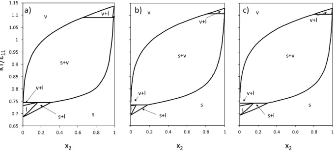
Fig. 3 shows the phase diagram for the binary LJ mixture with ₁₁/₂₂ 0.625 and

95 . 0 / ₂₂

11  

 . The MC simulation phase diagram (a) presents two SLVE temperatures. The LJ

SLV-EoS with null binary interaction parameters reproduces qualitatively the MC simulation results, but the SVE region exists in a wider temperature range (b). As explained above, this is because of the different representation of the pure fluid phase equilibrium between MC simulation [8] and reference 11 and 12 (LJ SLV-EoS reproduces phase equilibrium of reference 11 and 12). The LJ SLV-EoS model with regressed binary interaction parameters allows improving the composition of the liquid and solid phases on the SLVE at low temperature (c).

Fig. 4 shows the phase diagram for the binary LJ mixture with 11/22 1 and 11/22 0.95.

The MC simulation phase diagram (a) presents a SL azeotrope. The LJ SLV-EoS with null binary interaction parameters gives a solid solution with a very narrow SLE loop (b). In other words, the liquid phase is never stable for temperatures lower than the lowest melting temperature of the pure fluids. The LJ SLV-EoS model with regressed binary interaction parameters, see Tab. 2, allows representing the SL azeotrope.

The MC simulation phase diagram for the binary LJ mixture with ₁₁/₂₂ 1.6 and

95 . 0 / ₂₂

11  

 presents two SLVE lines, and is symmetrical to the diagram of Fig. 3a. The LJ

(13)

12 The LJ SLV-EoS model with regressed binary interaction parameters improves the values of the composition of the liquid and solid phases on the SLVE at low temperature. Because these diagrams are qualitatively similar to the diagrams in Fig. 3, graphs have not been presented, while binary interaction parameters are presented in Tab. 2.

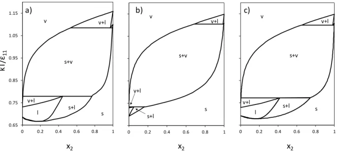
Fig. 5 shows the phase diagrams for the binary LJ mixture with ₁₁/₂₂ 0.625 and

9 . 0 / ₂₂

11  

 . The MC simulation phase diagram (a) presents two SLVE lines, with a SL

azeotrope at low temperatures. The LJ SLV-EoS with null binary interaction parameters gives a SVE region with a wider extension in temperature and does not represent the SL azeotrope. The LJ SLV-EoS model with regressed binary interaction parameters improves the temperatures at which SLVE exists and the composition of the liquid and solid phases on the SLVE at low temperature (c). Furthermore, the SL azeotrope at low temperatures in represented.

The MC simulation phase diagram for the binary LJ mixture with 11/22 1 and 11/22 0.9

presents a SL azeotrope at low temperatures. The difference between the azeotrope temperature and the melting temperature of the pure solids is much lower than in Fig. 4a, even if the diagram is qualitatively similar. As in the case of Fig. 4b, the LJ SLV-EoS with null binary interaction parameters gives a solid solution phase diagram. The LJ SLV-EoS model with regressed binary interaction parameters allows representing the SL azeotrope. The azeotrope temperature is also in good agreement with the MC simulation results. Figures are not presented for this case, because it is qualitatively similar to the case shown in Fig. 4.

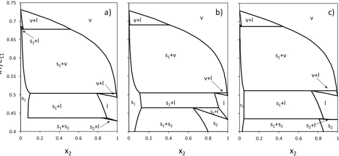
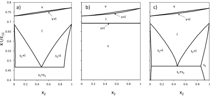
Fig. 6 shows the phase diagram for the binary LJ mixture with ₁₁/₂₂ 1.6 and ₁₁/₂₂ 0.9.

The MC simulation phase diagram (a) presents one S1S2LE line and two SLVE lines. The LJ

SLV-EoS with null binary interaction parameters predicts a S1S2LE at higher temperatures with

(14)

13

S1LE region. Furthermore, composition x2 in solid 2 of the S1S2LE is much lower than the

corresponding composition calculated by MC simulation. The LJ SLV-EoS model with regressed binary interaction parameters allows improving the representation of both the temperature and the compositions of the three-phase lines (c).

Fig. 7 shows the phase diagram for the binary LJ mixture with ₁₁/₂₂ 0.625 and

85 . 0 / ₂₂

11  

 . The MC simulation phase diagram (a) presents one S1S2LE line and two SLVE

lines. Eutectic behavior is present at low temperatures. The LJ SLV-EoS with null binary

interaction parameters does not predict the S1S2LE and the eutectic (b). The predicted phase

diagram is qualitatively correct at high temperatures, but at low temperatures the results are not in agreement with the MC simulation data. The LJ SLV-EoS model with regressed binary

interaction parameters allows representing the S1S2LE and the eutectic (c), allowing a qualitative

correct representation of the phase diagram produced by MC simulation.

Fig. 8 shows the phase diagram for the binary LJ mixture with 11/22 1 and 11/22 0.85.

The MC simulation phase diagram (a) presents eutectic behavior. The LJ SLV-EoS with null binary interaction parameters does not predict the eutectic (b); instead, a solid solution is predicted. The LJ SLV-EoS model with regressed binary interaction parameters allows

representing the eutectic (c). The S1S2LE temperature is in agreement with the one predicted by

MC simulation.

Fig. 9 shows the phase diagram for the binary LJ mixture with ₁₁/₂₂ 1.6 and ₁₁/₂₂ 0.85.

The MC simulation phase diagram presents a S1S2LE with eutectic behavior and two SLVE lines

(a). The LJ SLV-EoS with null binary interaction parameters does not predict the eutectic (b);

furthermore it predicts a S1S2LE temperature higher than the melting temperature of component

(15)

14 solid phase. Instead, the LJ SLV-EoS model with regressed binary interaction parameters allows representing the eutectic (c). The three-phase equilibrium temperatures and compositions are in good agreement with the MC simulation.

The MC simulation phase diagram for the binary LJ mixture with ₁₁/₂₂ 0.625 and

1 / ₂₂

11  

 presents two SLVE temperatures. The LJ SLV-EoS with null binary interaction

parameters reproduces qualitatively the MC simulation results. With respect to this last, the LJ SLV-EoS model with regressed binary interaction parameters allows improving the representation of the composition of the liquid phases on the SLVE line at low temperature.

Figures for this case are very similar to the figures presented for the case 11/22 0.625 and

95 . 0 / 22 11  

 (see Fig. 3) and therefore they have not been presented.

The MC simulation phase diagram for the binary LJ mixture with 11/22 1.6 and 11/22 1

presents two SLVE temperatures. The LJ SLV-EoS with null binary interaction parameters reproduces qualitatively the MC simulation results. The use of binary interaction parameters in the LJ SLV-EoS changes only slightly the obtained phase diagram. The phase diagrams concerning this case are qualitatively similar to the diagrams presented in Fig. 3.

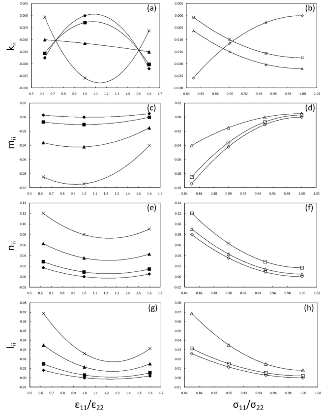
Fig. 10 shows the binary interaction parameters used in Figs. 3-9 plotted as function of the ratio

22 11/

 and ₁₁/₂₂. In particular, Figs. 10(a), (c), (e), and (g) show the dependence of kij, mij,

nij, and lij from 11/22 at constant 11/22; Figs. 10(b), (d), (f), and (h) show the dependence of

(16)

15

4. Conclusions

The equation of state for solid, liquid, and vapor phases, recently proposed by A. Yokozeki, has been applied to Lennard-Jones fluids. The LJ SLV-EoS has been compared with molecular simulation results for pure fluids and binary mixtures. The representation of pure fluids phase diagram is satisfactory for VLE, SLE, and SVE.

Phase diagrams for binary LJ mixtures have been produced for ₁₁/₂₂ ranging from 0.85 to 1,

and ₁₁/₂₂ ranging from 0.625 to 1.6 for a reduced pressure P* = 0.002. In this range of

parameters, three types of solid-liquid equilibria are encountered: solid solutions, solid-liquid azeotrope, and eutectic with partial immiscibility. The LJ SLV-EoS with null binary interaction parameters never predicts a liquid phase stable at temperatures lower than the lowest melting

temperature of the pure solids for the whole range of 11/22 and 11/22. This condition is

necessary for having eutectic or solid-liquid azeotrope. Another interpretation of this behavior is that the solid-solid miscibility is always over-estimated by the LJ SLV-EoS with null binary interaction parameters.

For representing qualitatively the evolution of the MC simulation phase diagrams, all the four interaction parameters were used. The reason is that the SLV-EoS describes the solid phase as a high-density liquid phase, and mixing rules for the solid and the liquid phases have the same form. For this reason, the miscibility of the solid phases is overestimated. For decreasing the mutual solubility of the solid phases, binary interaction parameters must be used. As a consequence, the LJ SLV-EoS is mainly adapted to the representation of the phase equilibrium of small, simple molecules, showing partial or total solubility in the solid phases.

(17)

16

Binary interaction parameters in the LJ SLV-EoS have been obtained as function of ε11/ε22 and

σ11/σ22, allowing predicting the phase behavior of other LJ mixtures (not used in the parameters

regression procedure) only knowing the LJ parameters of the pure components.

At the same time, phase diagrams for mixtures of real (LJ-like) fluids can be qualitatively predicted once the LJ parameters for the fluids are known. This result is also useful for interpreting the type of phase diagram of mixtures of simple molecules when only few data are available. As future work, the procedure developed in this work for estimating binary interaction parameters of the SLV-EoS for simple molecules will be applied for predicting the phase diagrams of mixtures of real fluids.

Acknowledgements

Authors are thankful to Air Liquide, Centre de Recherche Claude Delorme (France), for the financial support to the PhD thesis of M. Campestrini.

Nomenclature

List of symbols

a Equation of state parameter [J*m3/mol2]

a0 Parameter in Eq. (4)

(18)

17

b0 Parameter in Eq. (5)

b1 Parameter in Eq. (5)

b2 Parameter in Eq. (5)

c Liquid covolume [m3/mol]

d Equation of state parameter [m3/mol]

f Fugacity

B

k Boltzmann constant: 1.380648813×10-23 [J/K]

k Binary interaction parameter

l Binary interaction parameter

m Binary interaction parameter

n Binary interaction parameter

N Number of components in the mixture

NA Avogadro number: 6.022141793×1023 [mol-1]

P Pressure [Pa]

R Gas constant: R = NA·kB [J/(mol·K)]

T Temperature [K]

v Molar volume [m3/mol]

Greek letters

ε Well depth in Lennard-Jones potential [J]

σ Collision diameter in Lennard-Jones potential [m] φ Fugacity coefficient

Subscript

c Related to the critical point

(19)

18

j Relative to the substance j

ij Relative to the interaction between substance i and the substance j

ji Relative to the interaction between substance j and the substance i

ii Relative to the self-interaction for the substance i (considered null in this work)

ms Obtained by molecular simulation

EoS Obtained by the equation of state (LJ SLV-EoS)

ob Objective (function)

SLE Solid-liquid equilibrium

VLE Vapor-liquid equilibrium

SVE Solid-vapor equilibrium

t Related to the triple point

Superscript

* Reduced

L Liquid phase

m Parameter in Eq. (5)

mix Relative to the mixture

n Parameter in Eq. (4)

S Solid phase

(20)

19

References

[1] M. Matsuoka, Bunri Gijutsu 7 (1977) 245-249.

[2] M. Matsuoka in: J. Garside, R.J. Davey, A. Jones (Eds.), Advances in Industrial

Crystallization, Butterworth-Heinemann Ltd., Oxford-London, 1991, pp. 229-224.

[3] J. Gmehling, B. Kolbe, Thermodynamik, second ed., VCH-Verlag, Weinheim, 1992.

[4] R. Heastie, Nature 176 (1955) 747-748.

[5] P. van’t Zelfde, M.H. Omar, H.G.M. le Pair-Schroten, Z. Dokoupil, Physica 38 (1968)

241-252.

[6] A. Yokozeki, Int. J. Thermophys. 24 (2003) 589-620.

[7] M.R. Hitchcock, C.K. Hall, J. Chem. Phys. 110 (1999) 11433-11444.

[8] M.H. Lamm, C.K. Hall, AIChE J. 47 (2001) 1664-1675.

[9] M.H. Lamm, C.K. Hall, Fluid Phase Equilib. 182 (2001) 37-46.

[10] M.H. Lamm, C.K. Hall, Fluid Phase Equilib. 194-197 (2002) 197-206. [11] A. Lotfi, J. Vrabec, J. Fischer, Mol. Phys. 76 (1992) 1319-1333. [12] M.A. Barroso, A.L. Ferreira, J. Chem. Phys. 116 (2002) 7145-7150.

(21)

20 L S+L S 0 xB 1 T a) Solid solution L S+L S 0 xB 1 T b) Azeotrope L L+SA SA+SB 0 x 1 T

c) Eutectic with partial immiscibility L+SB L L+SA SA+SB 0 xB 1 T

d) Eutectic with complete immiscibility L+SB L L+SA SA+C 0 xB 1 T

e) Peritectic with eutectic

L+SB L+C SB+C L L+SA SA+C 0 xB 1 T f) Molecular compound L+SB L+C SB+C

Figure 1. Types of solid–liquid phase diagrams identified by Matsuoka [1]: (a) solid solution, (b)

azeotrope, (c) eutectic with partial immiscibility, (d) eutectic with complete immiscibility, (e)

peritectic with eutectic, and (f) molecular compound. The phase diagrams are shown in the T-xB

plane where xB is the mole fraction of component B. L = liquid mixture of A and B, S = solid

solution of A and B, SA = solid solution rich in A, SB = solid solution rich in B, C = ordered solid

(22)

21 0.0001 0.001 0.01 0.1 1 10 100 0.5 1.0 1.5 2.0 P* T*

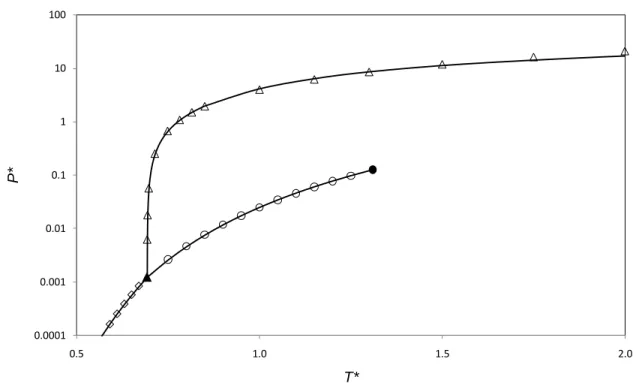
Figure 2. Reduced pressure, P*, versus reduced temperature, T*, diagram for the pure

Lennard-Jones fluid. Symbols represent molecular simulation results. ○: VLE [11]; ◊ SVE [12]; Δ: SLE

(23)

22 0.65 0.7 0.75 0.8 0.85 0.9 0.95 1 1.05 1.1 1.15 0 0.2 0.4 0.6 0.8 1 v s+v v+l v+l s+l s l 0.65 0.7 0.75 0.8 0.85 0.9 0.95 1 1.05 1.1 1.15 0 0.2 0.4 0.6 0.8 1 v s+v v+l v+l s+l s l 0.65 0.7 0.75 0.8 0.85 0.9 0.95 1 1.05 1.1 1.15 0 0.2 0.4 0.6 0.8 1 s+v v+l v+l s+l v s l b) a) c) x2 x2 x2 kT /ε11

Figure 3. Temperature vs. composition phase diagrams for Lennard-Jones binary mixtures with

22 11/

 = 0.625 and ₁₁/₂₂ = 0.95 at P* = 0.002. (a) MC simulation diagram from [8]; (b) LJ

SLV-EoS with null binary interaction parameters; (c) LJ SLV-EoS with regressed binary interaction parameters.

(24)

23 0.65 0.66 0.67 0.68 0.69 0.7 0.71 0.72 0.73 0.74 0.75 0 0.2 0.4 0.6 0.8 1 v v+l l s+l s 0.65 0.66 0.67 0.68 0.69 0.7 0.71 0.72 0.73 0.74 0.75 0 0.2 0.4 0.6 0.8 1 v v+l l s+l s 0.65 0.66 0.67 0.68 0.69 0.7 0.71 0.72 0.73 0.74 0.75 0 0.2 0.4 0.6 0.8 1 v+l s+l v l s b) a) c) x2 x2 x2 kT /ε11

22 11/

 = 1 and ₁₁/₂₂ = 0.95 at P* = 0.002. (a) MC simulation diagram from [8]; (b) LJ

SLV-EoS with null binary interaction parameters; (c) LJ SLV-SLV-EoS with regressed binary interaction parameters.

(25)

24 0.65 0.75 0.85 0.95 1.05 1.15 0 0.2 0.4 0.6 0.8 1 v v+l s+v v+l l s+l s 0.65 0.75 0.85 0.95 1.05 1.15 0 0.2 0.4 0.6 0.8 1 v v+l s+v v+l s+l s 0.65 0.75 0.85 0.95 1.05 1.15 0 0.2 0.4 0.6 0.8 1 v s l s+v v+l v+l s+l b) a) c) x2 x2 x2 kT /ε11

22 11/

(26)

25 0.4 0.45 0.5 0.55 0.6 0.65 0.7 0.75 0 0.2 0.4 0.6 0.8 1 v v+l s1+v v+l l s1+l s1+s2 s2+l s2 s1 0.4 0.45 0.5 0.55 0.6 0.65 0.7 0.75 0 0.2 0.4 0.6 0.8 1 v v+l s1+v v+l l s1+l s1+s2 s2+l s2 s1 0.4 0.45 0.5 0.55 0.6 0.65 0.7 0.75 0 0.2 0.4 0.6 0.8 1 v s1+s2 v+l s1+l s1+v s1+l v+l s1 l s2+l b) a) c) x2 x2 x2 kT /ε11

22 11/

(27)

26 0.5 0.6 0.7 0.8 0.9 1 1.1 1.2 0 0.2 0.4 0.6 0.8 1 v _v+l s2+l s2+v v+l s2+l l s1+l s1+s2 s1 s2 0.5 0.6 0.7 0.8 0.9 1 1.1 1.2 0 0.2 0.4 0.6 0.8 1 v _v+l s+v s s+l 0.5 0.6 0.7 0.8 0.9 1 1.1 1.2 0 0.2 0.4 0.6 0.8 1 v s1+s2 s2+l l v+l v+l s2+l s2 s1+l s2+v b) a) c) x2 x2 x2 kT /ε11

22 11/

(28)

27 0.4 0.45 0.5 0.55 0.6 0.65 0.7 0.75 0.8 0 0.2 0.4 0.6 0.8 1 v v+l l s1+l s2+l s1+s2 s2 0.4 0.45 0.5 0.55 0.6 0.65 0.7 0.75 0.8 0 0.2 0.4 0.6 0.8 1 v v+l l s+l s 0.4 0.45 0.5 0.55 0.6 0.65 0.7 0.75 0.8 0 0.2 0.4 0.6 0.8 1 v l v+l s1+s2 s1+l s2+l b) a) c) x2 x2 x2 kT /ε11

22 11/

 = 1 and ₁₁/₂₂ = 0.85 at P* = 0.002. (a) MC simulation diagram from [8]; (b) LJ

(29)

28 0.4 0.45 0.5 0.55 0.6 0.65 0.7 0.75 0 0.2 0.4 0.6 0.8 1 v+l s1+v v+l s1+l s1+s2 s2+l v l 0.4 0.45 0.5 0.55 0.6 0.65 0.7 0.75 0 0.2 0.4 0.6 0.8 1 v+l s1+v v+l s1+l s1+s2 s2+l v l 0.4 0.45 0.5 0.55 0.6 0.65 0.7 0.75 0 0.2 0.4 0.6 0.8 1 v l s2+l s1+s2 s1+l s1+v v+l v+l b) a) c) x2 x2 x2 kT /ε11

22 11/

 = 1.6 and 11/22 = 0.85 at P

*

= 0.002. (a) MC simulation diagram from [8]; (b) LJ SLV-EoS with null binary interaction parameters; (c) LJ SLV-EoS with regressed binary interaction parameters.

(30)

29

m

ij

n

ij

l

ij

ε

₁₁

/ε

₂₂

σ

₁₁

/σ

₂₂

k

ij -0.030 -0.025 -0.020 -0.015 -0.010 -0.005 0.000 0.005 0.84 0.86 0.88 0.90 0.92 0.94 0.96 0.98 1.00 1.02 (b) -0.10 -0.08 -0.06 -0.04 -0.02 0.00 0.02 0.84 0.86 0.88 0.90 0.92 0.94 0.96 0.98 1.00 1.02 (d) -0.10 -0.08 -0.06 -0.04 -0.02 0.00 0.02 0.5 0.6 0.7 0.8 0.9 1.0 1.1 1.2 1.3 1.4 1.5 1.6 1.7 (c) -0.030 -0.025 -0.020 -0.015 -0.010 -0.005 0.000 0.005 0.5 0.6 0.7 0.8 0.9 1.0 1.1 1.2 1.3 1.4 1.5 1.6 1.7 (a) -0.02 0.00 0.02 0.04 0.06 0.08 0.10 0.12 0.14 0.5 0.6 0.7 0.8 0.9 1.0 1.1 1.2 1.3 1.4 1.5 1.6 1.7 (e) -0.02 0.00 0.02 0.04 0.06 0.08 0.10 0.12 0.14 0.84 0.86 0.88 0.90 0.92 0.94 0.96 0.98 1.00 1.02 (f) -0.01 0.00 0.01 0.02 0.03 0.04 0.05 0.06 0.07 0.08 0.5 0.6 0.7 0.8 0.9 1.0 1.1 1.2 1.3 1.4 1.5 1.6 1.7 (g) -0.01 0.00 0.01 0.02 0.03 0.04 0.05 0.06 0.07 0.08 0.84 0.86 0.88 0.90 0.92 0.94 0.96 0.98 1.00 1.02 (h)

Figure 10. Dependence of the binary interaction parameters kij, mij, nij, lij from 11/22 and 22

11/

 . (─▲─):11/22 = 0.9; (─×─):11/22 = 0.85; (─■─):11/22 = 0.95;

(─

♦

─):11/22 = 1; (─Δ─):11/22 = 1.6; (─◊─): 11/22 = 1; (─□─):11/22 = 0.625; (──):

(31)

30

Table 1. Parameters of the SLV-EoS in reduced variables, eqs (2), (4), and (5).

Parameter Value Units

a0 2.39647×10-1 - a1 4.67098×102 - a2 4.34036 - n 3.03527×10-1 - b0 1.27853 - b1 -3.23646×10-1 - b2 1.99173 - m 1.39554 - c* 1.33224 - d* 1.29463 - NA 6.022141793×1023 mol-1 kB 1.380648813×10-23 J/K

(32)

31

Table 2. Binary interaction parameters used for graphs (c) in Figures 3 to 9.

22 11/  ₁₁/₂₂ k₁₂k₂₁ l₁₂ l₂₁ m₁₂ m₂₁ n₁₂ n₂₁ 0.625 0.95 -1.563×10-2 1.475×10-2 -6.75×10-3 2.85×10-2 1 0.95 -2.875×10-3 2.875×10-3 -1.05×10-2 8.875×10-3 1.6 0.95 -2.025×10-2 5.25×10-3 0 1.45×10-2 0.625 0.9 -1×10-2 3.5×10-2 -3.6×10-2 6.3×10-2 1 0.9 -1.15×10-2 1.15×10-2 -4.2×10-2 3.55×10-2 1.6 0.9 -1.5×10-2 1.5×10-2 -1.5×10-2 4.3×10-2 0.625 0.85 -6.25×10-4 6.875×10-2 -8.475×10-2 1.205×10-1 1 0.85 -2.588×10-2 2.5875×10-2 -9.45×10-2 7.9875×10-2 1.6 0.85 -6.25×10-3 3.125×10-2 -4×10-2 9.05×10-2 0.625 1 -1.75×10-2 8×10-3 3×10-3 1.7×10-2 1.6 1 -2.2×10-2 2×10-3 5×10-3 5×10-3

(33)

32

Table 3. Abbreviations used in Figures 3 to 9.

Abbreviations Subscripts Meaning

s solid phase l liquid phase v vapor phase s+l solid-liquid equilibrium s+v solid-vapor equilibrium l+v vapor-liquid equilibrium

1 phase rich in component 1