HAL Id: inria-00131287
https://hal.inria.fr/inria-00131287v2
Submitted on 27 Feb 2007
HAL is a multi-disciplinary open access
archive for the deposit and dissemination of
sci-entific research documents, whether they are
pub-lished or not. The documents may come from
teaching and research institutions in France or
abroad, or from public or private research centers.
L’archive ouverte pluridisciplinaire HAL, est
destinée au dépôt et à la diffusion de documents
scientifiques de niveau recherche, publiés ou non,
émanant des établissements d’enseignement et de
recherche français ou étrangers, des laboratoires
publics ou privés.
Fast Non Local Means Denoising for 3D MR Images
Pierrick Coupé, Pierre Yger, Christian Barillot
To cite this version:
Pierrick Coupé, Pierre Yger, Christian Barillot. Fast Non Local Means Denoising for 3D MR Images.
9th International Conference on Medical Image Computing and Computer-Assisted Intervention, Oct
2006, Copenhagen, Denmark, pp.33-40, �10.1007/11866763_5�. �inria-00131287v2�
Fast Non Local Means Denoising
for 3D MR Images
Pierrick Coup´e1
, Pierre Yger1,2, Christian Barillot1
1 Unit/Project VisAGeS U746, INSERM - INRIA - CNRS - Univ-Rennes 1,
IRISA campus Beaulieu 35042 Rennes Cedex, France
2ENS Cachan, Brittany Extension - CS/IT Department 35170 Bruz, France
{pcoupe,pyger,cbarillo}@irisa.fr, http://www.irisa.fr/visages
Abstract. One critical issue in the context of image restoration is the problem of noise removal while keeping the integrity of relevant image information. Denoising is a crucial step to increase image conspicuity and to improve the performances of all the processings needed for quan-titative imaging analysis. The method proposed in this paper is based on an optimized version of the Non Local (NL) Means algorithm. This approach uses the natural redundancy of information in image to remove the noise. Tests were carried out on synthetic datasets and on real 3T MR images. The results show that the NL-means approach outperforms other classical denoising methods, such as Anisotropic Diffusion Filter and Total Variation.
1
Introduction
Image processing procedures needed for fully automated and quantitative anal-ysis (registration, segmentation, visualization) require to remove noise and arti-facts in order to improve their performances. One critical issue concerns therefore the problem of noise removal while keeping the integrity of relevant image in-formation. This is particularly true for various MRI sequences especially when they are acquired on new high field 3T systems. With such devices, along with the improvement of tissue contrast, 3T MR scans may introduce additive arti-facts (noise, bias field, geometrical deformation). This increase of noise impacts negatively on quantitative studies involving segmentation and/or registration procedures. This paper focuses on one critical aspect, image denoising, by in-troducing a new restoration scheme in the 3D medical imaging context. The proposed approach is based on the method originally introduced by Buades et
al.[2] but with specific adaptations to medical images. To limit a highly
expen-sive computational cost due to the size of the 3D medical data, we propose an optimized and parallelized implementation.
The paper is structured as follows: Section 2 presents a short overview of the Non Local (NL) means algorithm, Section 3 describes the proposed method with details about the original contribution, and Section 4 shows a comparative validation with respects to other well established denoising methods, and results obtained on a 3T MR scanner.
2
The Non Local Means algorithm
First introduced by Buades et al. in [2], the Non Local (NL) means algorithm is based on the natural redundancy of information in images to remove noise. This filter allows to avoid the well-known artifacts of the commonly used neigh-borhood filters [4]. In the theoretical formulation of the NL-means algorithm, the restored intensity of the voxel i, N L(v)(i), is a weighted average of all voxel intensities in the image I. Let us denote:
N L(v)(i) =X
j∈I
w(i, j)v(j) (1)
where v is the intensity function and thus v(j) is the intensity at voxel j and w(i, j) the weight assigned to v(j) in the restoration of voxel i. More precisely, the weight quantifies the similarity of voxels i and j under the assumptions that
w(i, j) ∈ [0, 1] and Pj∈Iw(i, j) = 1. The original definition of the NL means
algorithm considers that each voxel can be linked to all the others, but practically the number of voxels taken into account in the weighted average can be restricted
in a neighborhood that is called in the following “search volume” Vi of size
(2M +1)3
, centered at the current voxel i. In this search volume Vi, the similarity
between i and j depends on the similarity of their local neighborhoods Niand Nj
of size (2d+1)3
(cf Fig. 1). For each voxel j in Vi, the averaged Euclidean distance
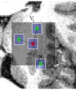
Fig. 1.2D illustration of the NL-means principle. The restored value of voxel i (in red) is a weighted average of all intensities of voxels j in the search volume Vi, according to
the similarity of their intensities neighborhoods v(Ni) and v(Nj).
k − k2
2,a defined in [2], is computed between v(Nj) and v(Ni). This distance is a
classical k − k2norm, convolved with a Gaussian kernel of standard deviation a,
and is a measure of the distortion between voxel neighborhood intensities. Then, 2
these distances are weighted by the function defined as follows: w(i, j) = 1 Z(i)e −kv(Ni)−v(Nj )k 2 2,a h2 (2)
where Z(i) is the normalization constant with Z(i) =Pjw(i, j), and h acts as
a filtering parameter.
In [2], Buades et al. show that for 2D natural images the NL-means algorithm outperforms the denoising state of art methods such as the Rudin-Osher-Fatemi Total Variation minimization procedure [8] or the Perona-Malik Anisotropic dif-fusion [7]. Nevertheless, the main disadvantage of the NL-means algorithm is the computational burden due to its complexity, especially on 3D data. Indeed, for each voxel of the volume, the algorithm has to compute distances between
the intensities neighborhoods v(Ni) and v(Nj) for all the voxels j contained in
V(i). Let us denote by N3
the size of the 3D image, then the complexity of the
algorithm is in the order of O((N (2M + 1)(2d + 1))3
). For a classical MR image data of 181 × 217 × 181 voxels, with the smallest possible value of d = 1, and
M = 5, the computational time reaches up to 6 hours. This time is far beyond
a reasonable duration expected for a denoising algorithm in a medical practice, and thus the reduction of complexity is crucial in the medical context.
3
Fast Implementation of the Non Local means algorithm
There are two main ways to address computational time for the NL-means: the decrease of computations performed and the improvement of the implementa-tion.
Voxel selection in the search volume One recent study [5] investigated
the problem of the computational burden with a neighborhoods classification. The aim is to reduce the number of voxels taken into account in the weighted average. In other words, the main idea is to select only the voxels j in V (i) that will have the highest weights w(i, j) in (1) without having to compute the
Euclidean distance between v(Ni) and v(Nj). Neglecting a priori the voxels
which are expected to have small weights, the algorithm can be speeded up, and the results are even improved (see Table 4.1). In [5], Mahmoudi et al. propose a method to preselect a set of the most pertinent voxels j in V (i). This selection
is based on the similarity of the mean and the gradient of v(Ni) and v(Nj):
intuitively, similar neighborhoods tend to have close means and close gradients.
In our implementation, the preselection of the voxels in Vi that are expected
to have the nearest neighborhoods to i is based on the first and second order
moments of v(Ni) and v(Nj). The gradient being sensitive to noise level, the
standard deviation is preferable in case of high level of noise. In this way, the maps of local means and local standard deviations are precomputed in order to avoid repetitive calculations of moments for one same neighborhood. The
selection tests can be expressed as follows: w(i, j) = 8 < : 1 Z(i)e − kv(Ni)−v(Nj )k22,a h2 if µ1< v(Ni) v(Nj)
< µ2 and σ12<var(v(Nvar(v(Nij)))) < σ
2 2
0 otherwise.
(3)
Parallelized computation Another way to deal with the problem of the
com-putational time required is to share the operations on several processors via a cluster or a grid. In fact, the intrinsic nature of the NL-means algorithm allows to use multithreading, and thus to parallelize the operations. We divide the vol-ume into sub-volvol-umes, each of them being treated separately by one processor. A server with eight Xeon processors at 3 GHz was used in our experiments.
4
Results
4.1 Validation on Phantom data set
In order to evaluate the performances of the NL-means algorithm on 3D T1
MR images, tests are performed on the Brainweb database1
[3] composed of 181 × 217 × 181 images. The evaluation framework is based on comparisons with
other denoising methods: Anisotropic Diffusion Filter (implemented in VTK2
) and the Rudin-Osher-Fatemi Total Variation (TV) approach [8]. Several criteria are used to quantify the performances of each method: the Peak Signal to Noise Ratio (PSNR) obtained for different noise levels, histogram comparisons between the denoised images and the “ground truth”, and finally the visual assessment. In the following, the noise is a white Gaussian noise, and the percent level is based on a reference tissue intensity, that is in this case the white matter. For the sake of clarity, the PSNR and the histograms are estimated by removing the background.
Peak Signal Noise Ratio A common factor used to quantify the differences
between images is the Peak Signal to Noise Ratio (PSNR). For images encoded on 8bits the PSNR is defined as follows:
P SN R= 20 log10
255
RM SE (4)
where the RMSE is the root mean square error estimated between the ground truth and the denoised image. As we can see on Fig. 2, our optimized NL-means algorithm produces the best values of PSNR whatever the noise level. In average, a gain of 2.6dB is observed compared to the best method among TV and Anisotropic Diffusion, and a gain of ' 1.2dB compared to the classical NL-means. The PSNR between the noisy images and the ground truth is called “No processing” and is used as the reference for PSNR before denoising.
1 http://www.bic.mni.mcgill.ca/brainweb/ 2 www.vtk.org
3 9 15 21 15 20 25 30 35 40
Noise level σ (in %)
PSNR (in dB) No Processing Anisotropic Diffusion Total Variation Classical NL−means Optimized NL−means
Fig. 2. PSNR values for the three compared methods for different levels of noise. The PSNR between the noisy images and the ground truth is called “No processing” and is used as the reference for PSNR before denoising. For each level of noise, the optimized NL-means algorithm outperforms the Anisotropic Diffusion method, the Total Variation method, and the classical NL-means.
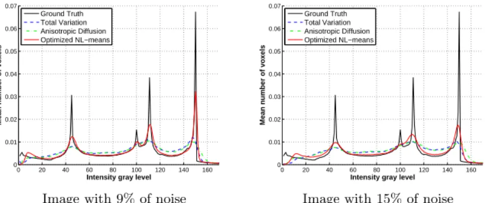
Histogram comparison To better understand how these differences in the
PSNR between the three compared methods can be explained, we compared the histograms of the denoised images with the ground truth. On Fig. 3 it is shown that the NL-means is the only method able to retrieve a similar histogram as the ground truth. The NL-means restoration distinguishes clearly the three main peaks representing the white matter, the gray matter and the cerebrospinal fluid. The sharpness of the peaks shows how the NL-means increases the contrasts between denoised biological structures (see also Fig. 4).
0 20 40 60 80 100 120 140 160 0 0.01 0.02 0.03 0.04 0.05 0.06 0.07
Intensity gray level
Mean number of voxels
Ground Truth Total Variation Anisotropic Diffusion Optimized NL−means
Image with 9% of noise
0 20 40 60 80 100 120 140 160 0 0.01 0.02 0.03 0.04 0.05 0.06 0.07
Intensity gray level
Mean number of voxels
Ground Truth Total Variation Anisotropic Diffusion Optimized NL−means
Image with 15% of noise
Fig. 3.Histograms of the restored images and of the ground truth. The histogram of the NL-means restored image clearly better fits to the ground truth one. Left: image with 9% of noise, Right: image with 15% of noise.
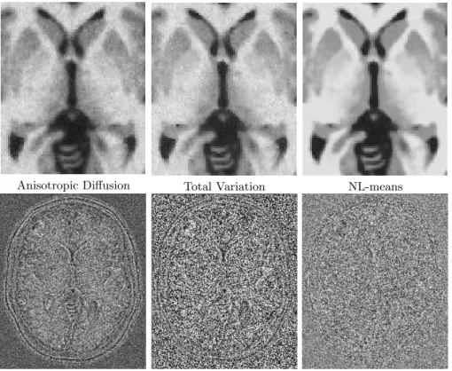
Visual assessment Fig. 4 shows the restored images and the removed noise
we can observe that the homogeneity in white matter is higher in the image denoised by the NL-means algorithm. Moreover, if we focus on the nature of the removed noises, it clearly appears that the NL-means restoration preserves better the high frequencies components of the image (i.e. edges).
Anisotropic Diffusion Total Variation NL-means
Fig. 4.Top: details of the Brainweb denoised images obtained via the three compared methods for a noise level of 9%. Bottom: images of the removed noise, i.e. the differ-ence between noisy images and denoised images, centered on 128. From left to right: Anisotropic Diffusion, Total Variation and NL-means.
Optimization contribution In all experiments, the typical values used for the
NL-means parameters are d = 1 (i.e Card(Ni) = 33), M = 5 (i.e Card(Vi) =
113
), µ1 = 0.95, µ2 = 1.05, σ
2
1 = 0.5, σ
2
2 = 1.5, and h is close to the standard
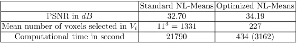
deviation of the added noise, influencing the smoothness of the global solution. To obtain a significant improvement in the results, d can be increased, but it implies to increase M yielding to a prohibitive computational time. Table 4.1 summarizes the influence of the restriction of the average number of voxels taken into account in the search volume (see (3)) and the parallelization of the imple-mentation. Those results demonstrate how the neighborhoods selection is useful for two reasons: the computational time is drastically reduced and the PSNR is even improved by the preselection of the nearest voxels while computing the
weighted averages. Combined with multithreading, these two optimizations lead
to an overall reduction of the computational time by a factor 21790
434 w 50. This
reduction factor is even more important when Card(Vi) and Card(Ni) (i.e M
and d) increase.
Standard NL-Means Optimized NL-Means
PSNR in dB 32.70 34.19
Mean number of voxels selected in Vi 113= 1331 227
Computational time in second 21790 434 (3162)
Table 1.Results obtained for standard and optimized NL-means implementations on a Brainweb T1 image of size 181 × 217 × 181 with 9% of noise (d = 1 and M = 5). The time shown for the standard NL-means is calculated on only one processor of the server described in 3. The time given for our optimized version corresponds to the time with the server, and the cumulative CPU time is shown between brackets.
4.2 Experiments on Clinical data
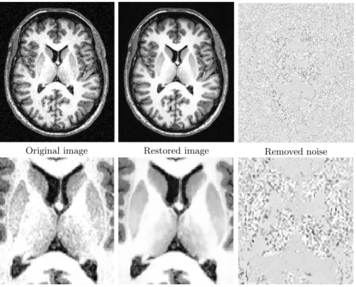
To show the efficiency of the NL-means algorithm on real data, tests have been performed on a high field MR system (3T). In these images, the gain in resolu-tion being obtained at the expense of an increase of the level of noise, the de-noising step is particularly important. The restoration results, presented in Fig. 5, show good preservation of the basal ganglia. Fully automatic segmentation and quantitative analysis of such structures are still a challenge, and improved restoration-schemes could greatly improve these processings.
5
Conclusion and further works
This paper presents an optimized version of the Non Local (NL) means al-gorithm, applied to 3D medical data. The validations performed on Brainweb dataset [3] bring to the fore how the NL-means denoising outperforms well estab-lished other methods, such as Anisotropic Diffusion [7] and Total Variation [8]. If the performances of this approach clearly appears, the reduction of its intrinsic complexity is still a challenging problem. Our proposed optimized implemen-tation, with voxel preselection and multithreading, considerably decreases the required computational time (up to a factor of 50). Further works should be pur-sued for comparing NL-means with recent promising denoising methods, such as Total Variation on Wavelet domains [6] or adaptative estimation method [1]. The impact of this NL-means denoising on the performances of post-processing algorithms, like segmentation and registration schemes need also to be further investigated.
References
1. J. Boulanger, Ch. Kervrann, and P. Bouthemy. Adaptive spatio-temporal restora-tion for 4d fluoresence microscopic imaging. In Int. Conf. on Medical Image Comput-ing and Computer Assisted Intervention (MICCAI’05), Palm SprComput-ings, USA, October 2005.
Original image Restored image Removed noise
Fig. 5.NL-means restoration of 3T MRI data of 2563 voxels with d = 1, M = 5 in
less than 10 minutes. From left to right: Original image, denoised image, and difference image centered on 128. The whole image is shown on top, and a detail is exposed on bottom.
2. A. Buades, B. Coll, and J. M. Morel. A review of image denoising algorithms, with a new one. Multiscale Modeling & Simulation, 4(2):490–530, 2005.
3. D. L. Collins, A. P. Zijdenbos, V. Kollokian, J. G. Sled, N. J. Kabani, C. J. Holmes, and A. C. Evans. Design and construction of a realistic digital brain phantom. IEEE Trans. Med. Imaging, 17(3):463–468, 1998.
4. J.S. Lee. Digital image smoothing and the sigma filter. Computer Vision, Graphics and Image Processing, 24:255–269, 1983.
5. M. Mahmoudi and G. Sapiro. Fast image and video denoising via non-local means of similar neighborhoods. IMA Preprint Series, 2052, 2005.
6. A. Ogier, P. Hellier, and C. Barillot. Restoration of 3D medical images with to-tal variation scheme on wavelet domains (TVW). In Proceedings of SPIE Medical Imaging 2006: Image Processing, San Diego, USA, February 2006.
7. P. Perona and J. Malik. Scale-space and edge detection using anisotropic diffusion. IEEE Trans. Pattern Anal. Mach. Intell., 12(7):629–639, 1990.
8. L. I. Rudin, S. Osher, and E. Fatemi. Nonlinear total variation based noise removal algorithms. Physica D, 60:259–268, 1992.