HAL Id: hal-01435089
https://hal.archives-ouvertes.fr/hal-01435089
Submitted on 13 Jan 2017HAL is a multi-disciplinary open access archive for the deposit and dissemination of sci-entific research documents, whether they are pub-lished or not. The documents may come from teaching and research institutions in France or abroad, or from public or private research centers.
L’archive ouverte pluridisciplinaire HAL, est destinée au dépôt et à la diffusion de documents scientifiques de niveau recherche, publiés ou non, émanant des établissements d’enseignement et de recherche français ou étrangers, des laboratoires publics ou privés.
for mixed-model machining on rotary transfer machine
Olga Battaïa, Alexandre Dolgui, Nikolai Guschinsky
To cite this version:
Olga Battaïa, Alexandre Dolgui, Nikolai Guschinsky. Integrated process planning and system configu-ration for mixed-model machining on rotary transfer machine. International Journal of Computer Inte-grated Manufacturing, Taylor & Francis, 2017, 30 (9), pp.910-925. �10.1080/0951192X.2016.1247989�. �hal-01435089�
International Journal of Computer Integrated Manufacturing
Received 18 Aug 2015, Accepted 09 Oct 2016, Published online: 01 Nov 2016
http://dx.doi.org/10.1080/0951192X.2016.1247989
Integrated process planning and system configuration for mixed-model
machining on rotary transfer machine
Olga Battaïa *, Alexandre Dolgui **, Nikolai Guschinsky***
* ISAE-Supaéro, Toulouse, France (e-mail: [email protected])
** École des Mines de Nantes, CNRS UMR6597 IRCCYN, F-44307 NANTES Cedex 3, France (e-mail: [email protected])
*** Operatoinal Research Laboratory, United Institute of Informatics Problems, Academy of Sciences, Minsk, Belarus (e-mail: [email protected])
Abstract: New generation of rotary transfer machines processing different models of parts is considered. In order to enhance the cost-effectiveness of mixed-model rotary transfer machines, the problems of process planning for the parts to be machined and the configuration of a rotary transfer machine are integrated in the same optimisation problem. This problem is modelled as a combinatorial optimization problem. The decisions to be taken simultaneously concern the orientation of parts for machining, the machining parameters for processing the parts as well as the configuration of machining units to be used at working positions of the machine. Constraints related to the design of such units – spindle heads, turrets – and working positions, as well as precedence constraints related to machining operations, are taken into account. The problem consists in minimizing an estimated cost of the rotary transfer machine, while reaching a given output and satisfying all the constraints. The proposed methods to solve the problem are based on its MIP formulation. The optimisation techniques are validated on an industrial case study. Numerical experiments evaluate the efficiency of the approach against the variety of parts to be produced.
Keywords: Rotary machine, Product variety, Machine engineering, Production system design, Integrated process planning and system configuration, Line design and balancing, Combinatorial design, Combinatorial optimization, Industrial case study.
1. INTRODUCTION
Within the today’s context of increasing demand and product diversification, companies must be able to adapt their manufacturing systems for high variety production in order to profitably produce in small quantities different models of products. Mixed-model production is the practice of processing products without changeovers in the manufacturing system (Rabbani et al., 2014). Such a production mode poses new challenges in production system design, planning and management. In order to be cost-efficient several decision problems have to be considered jointly (Leonesio et al, 2013) such as process planning, system configuration and scheduling. In literature, each of these decision problems has attracted a large amount of research interest (Xu et al., 2011, Battaïa et al. 2012b, Guschinskaya et al., 2009, Dolgui et al., 2008). However, conventionally they have been performed sequentially (Lv and Qiao, 2014). Under the
modern production constraints and global competition, the strong dependence between these issues and its influence on the profitability of product manufacturing, resource utilisation and product delivery time cannot be ignored anymore. The growing amount of research work in the direction of joint consideration of these problems proves the importance of such an integrated approach.
It should be noted that the most advanced integration is currently realized between process planning and scheduling (Phanden et al. 2013; Bensmaine et al. 2014). The primary goal of process planning is to specify raw materials or components, processes and operations needed to convert a part from its raw material to the finished form (Yin et al., 2014). Scheduling receives process plans as its input and defines an order of processing the operations on machines while satisfying the precedence relations given in process plans. Scheduling is bound by process sequencing instructions given by the process plan and constrained by time-phased availability of production resources (Li and McMahon, 2007). However, even if a great research effort was dedicated to the integration of process planning and scheduling since the pioneer study by Chryssolouris et al. (1985), it still remains of limited functionality or compensated in computational efficiency due to the NP-hard nature of both problems (Mohapatra et al. 2014). The existing approaches for these two methods are broadly categorized into two types: the progressive/enumerative approach and the simultaneous/centralised approach. A comprehensive state-of-the-art review on the integration of process planning and scheduling has been recently realized by Phanden et al. (2011).
The configuration of machine tools and process planning problems are also traditionally managed as independent stages, where the process plan is designed by considering a number of machine tool solutions available from catalogue. Despite the fact that this strategy presents a number of disadvantages in terms of process results and machine capabilities fully exploitation, the integration of these decision problems has been rarer considered in the academic literature. Szadkowski (1971) has proposed one of the first models to optimize process plans for mass production taking into account combinatorial aspects and machining constraints. A graph approach for optimisation of mass production rotary transfer machines was proposed by Dolgui et al. (2009). A decision support system for design of mass production machining lines composed of stations with rotary or mobile table was developed by Battaïa et al. (2012a). This decision system included modules for part designing, process planning, system configuration and system cost optimisation. An integrated approach for jointly configuring machine tools and process planning with the objective to optimize the production costs was developed by Leonesio et al. (2013). The problem of combinatorial customization of automated production lines with rotary transfer and turrets was addressed by Battaïa et al. (2014a). Integrated configurable equipment selection and line balancing for mass production with serial–parallel machining systems was considered by Battaïa et al. (2014b). The studies considering reconfiguration of machining systems when it is necessary to integrate new parts to be machined requires also solving NP-hard optimization problems. For the case of mass production, where the integration of new parts is not effortless, optimisation techniques were proposed by Makssoud et al. (2014). To improve the flexibility of existing machining systems, several studies were conducted by Terkaj et al. (2009, 2010) and Copani et al (2015), Copani and Rosa (2015). Tolio and Urgo (2013) have proposed a mathematical model to assess the reconfiguration cost for flexible transfer lines. Variety-oriented design of rotary machining systems used for family part production was discussed by Battaïa et al. (2015).
Since no model available in the literature can be applied for the integrated process planning and system configuration for mixed-model machining on a rotary transfer machine, this paper develops such an optimisation model and evaluates it on an industrial case study.
The rotary transfer machine studied in this paper is used to produce simultaneously d0 types of parts. Such
machines are multi-positional, i.e. the parts are sequentially machined on m0 (1, 2, …, m0) working
unloading finished parts. It is assumed that the parts are loaded in sequence =(1, 2, …,0) where
i{0, 1, 2, …, d0}, i=1, 2, …, 0, 0 is multiple to m0+1 and i=0 means that no part is loaded. Using
sequence one can define in one-to-one manner function (i,k) of part number at the k-th working position each time when machining part i i.e.:
otherwise. , , if , ) , ( ) , mod( 0 0 0 0 0 k m i k m i i m k k i
At each working position, several machining units (spindle heads or turrets) can be installed to execute the operations assigned to this position. There are verical and horizontal units to process vertivally or horizontally, respectively. A turret holds several machining tools which are applied to the parts to be machined sequentially. A horizontal turret (spindle head) can work in parallel with a vertical spindle head (but not a turret) to access to different sides of parts at a working position. A vertical spindle head can be common for several working positions, i.e. can execute simultaneously operations on all these working positions. However, only one vertical turret can be mounted at one position or one common vertical spindle head can be installed for all working positions. Only one horizontal spindle head or turret can be used per position. For example, the rotary transfer machine in Fig. 1 has one vertical spindle head common for position 1,3,4,5, two horizontal turrets on position 1 and 3, and one horizontal spindle head on position 4.
Fig. 1. A rotary transfer machine with turrets
The rest of paper is organized as follows. Section 2 describes the decision variables and input data for the joint process planning and system configuration problem for mixed-model machining on a rotary transfer machine. Sections 3 provides a mathematical model for the considered combinatorial optimization problem. An industrial example is presented in Section 4. The results of numerical experiments are given and analyzed in Section 5. Concluding remarks are reported in Section 6.
2. PROBLEM STATEMENT 2.1. Notations and definitions
Let Nd be the set of machining operations needed for machining elements of the d-th part, d=1, 2, …, d0,
located on nd sides and N , s=1, 2, …, nsd d, be a subset of opertations for machining elements of the s-th
Turret Horizontal multi- spindle head Turret Common vertical multi-spindle head
side of the part. Part d can be located in different orientations, the set of all possible orientations is H(d) is known. Part orientation is done at zero position and still the same for all working positions. Elements of no more than one side can be machined by vertical spindle head or turret. All elements of other sides of the part have to be assigned to horizontal spindle heads or turrets. H(d) can be represented by matrix of dimension rdxnd where hrs(d) is equal j, j=1,2 if the elements of the s-th side of the part d can be machined
by spindle head or turret type j. Let N= 0
1
d d
Nd. All operations pN are characterized by the following parameters:
- length (p) of the working stroke for operation pN, i.e. the distance to be run by the tool in order to complete operation p;
- range [γ1(p), γ2(p)] of feasible values of feed rate which characterizes the machining speed;
- set H(p) of feasible orientations of the part (indexes r{1, 2, …, rd} of rows of matrix H(d)) for
execution of operation pN by spindle head or turret of type j (vertical if hsd rs(d)=1 and horizontal if
hrs(d)=2).
Let subset Nk, k=1,...,m, contains the operations from set N assigned to the k-th working position.
Let sets Nk1 and Nk2 be the sets of operations assigned to working position k that are concerned by vertical
and horizontal machining, respectively.
Finally, let bkj be the number of machining modules (not more than b0) of type j (vertical if j=1 or
horizontal if j=2) installed at the k-th working position. Subsets Nkjl, l=1,...,bkj contain the operations from
set Nkj assigned to the same machining module.
The machining process imposes numerous constraints that have to be taken into account both for process planning and machining units’ configuration. In the literature, these constraints are commonly divided in the following categories (Battaïa and Dolgui, 2013).
Since the machining operations naturally have precedence relationships, they have to be taken into account on the process planning step. They are expressed by a directed graph GOR=(N,DOR) where an arc (p,q)DOR if and only if operation p has to be executed before operation q. It should be noted that if such operations p and q belong to different sides of the part then they cannot be executed at the same position. Tolerance constraints impose to execute certain operations at the same working position, by the same turret, by the same spindle head or even by the same spindle (for different parts). Such inclusion constraints are modeled by undirected graphs GSP=(N,ESP), GST=(N,EST), GSM=(N,ESM) and GSS=(N,ESS), where edge (p,q)ESS ((p,q)ESM, (p,q)EST, (p,q)ESP) if and only if operations p and q must be executed by the same spindle, machining module, turret, or at the same position, respectively.
On contrary, certain operations cannot be performed at the same working position, by the same turret or by the same spindle head for such evident reasons as tool intersections, impossibility of tool location in spindle head, turret, etc. These exclusion constraints are modeled by undirected graphs GDM=(N,EDM), GDT=(N,EDT), and GDP=(N,EDP), where edge (p,q)EDM ((p,q)EDT), (p,q)EDP)) if and only if operations p and q cannot be executed by the same machining module, turret, or at the same position, respectively.
The configuration of each machining unit depends on the operations assigned to it. The assignment of operations together, to be executed by the same machining unit, impose additional constraints on the choice of the cutting parameters. The choice of these parameters influences the machining time for each particular part and the makespan for completing all parts.
Let P=<P1,...,Pk,...,Pm0> is a design decision with Pk=(P1k11,P2k11,...,Pd0k11,…,P1k1bk1, P2k1bk1,…,Pd0k1bk1, 21 1k P ,P2k21,...,Pd0k21,…,P1k2bk1,P2k2bk1,…,Pd0k2bk1), Pdkjl=(Ndkjl,Гdkjl), Pdkj=(Pdkjl| l=1,…,bkj), Pdk=(Pdkj|j=1,2), and Nj = 0 0 1 1 1 d d m k b l dkjl kj N , j=1,2. 2.2. Machining time
The execution time tb(Pdkjl) of all operations from Ndkjl with a feed per minute Гdkjl[max{γ1(p)|pNdkjl},
min{γ2(p)|pNdkjl}] is equal to
tb(Pdkjl)=L(Ndkjl)/Гdkjl+a,
where L(Ndkjl)=max{(p)|pNdkjl}, and a is an additional constant time for advance and disengagement of
tools.
We assume that if a turret of type j is installed at k-th position, then the execution time of all operations from Ndkjl is equal to th(Pdkj)=gbkj + kj b l 1 tb(Pdkjl), |j=1, 2,
where g is an additional fixed time for one rotation of turret.
If the spindle head is installed, then th(Pdkj)= tb(Pdkjl), |j=1,2. If all Ndkjl are empty, then th(Pdkj)=0.
The execution time tp(Pdk) is defined as
tp(Pdk)=r+max{th(Pdkj)|j=1,2},
where r is an additional constant time for table rotation.
The time T(P) of execution of all corresponding operations after 0 turns of rotary table is defined as
follows T(P)=
0 1 i max{tp(P(i,k)k)|k=1,,m0}.We assume that the objective productivity is provided, if the total time T(P) does not exceed a given available time T0.
Let C1, C2, C3, and C4 be the relative costs for one position, one turret, one machining module of a turret,
and one horizontal spindle head, respectively.
Since a vertical spindle head (if it presents) is common for several positions, its size (and therefore the cost) depends on the number of positions to be covered. Let kminh and kmaxh be the minimal and maximal position number for positions covered by a common vertical spindle head. Then, the cost of such a spindle head can be estimated as C4+(kmaxh -kminh )C5, where C5 is the relative cost for covering one
additional position by a vertical spindle head.
The cost of a vertical turret can be estimated as C2+C3bk1.
In the similar way, the cost C(bk2) for performing set of operations Nk2 by associated bk2 machining
C(bk2) = . 1 if , 1 if , 0 if 0 2 2 3 2 2 4 2 k k k k b b C C b C b
The machine cost Q(P) is calculated as the total cost of all equipment used, i.e.
) )( | (| )) | (| 1 |)( (| ) ( 2 3 1 1 12 1 12 1 4 1 0 0 k m k k m k k sign N C C b N sign sign C m C P Q N
0 1 2 min max 5( ) ( ) m k k h h k C b k Cwhere sign(a) = 1 if a > 0, and sign(a) = 0 if a 0. The studied problem is to determine:
a) an orientation for each part to be produced;
b) an assignment of operations from set N into subsets Nkjl, k=1,...,m0, j=1,2, l=1,,bkj to be
performed by machining module l of type j at working position k;
c) a feed per minute Xdkjl employed for each set of operations Ndkjl= NkjlNd, d=1,...,d0, k=1,...,m0,
j=1,2, l=1,, bkj
in such a way that the machine cost Q(P) is as small as possible and all given constraints are respected.
Based on matrices H(d), d=1, 2, …, d0, we can build matrix H of dimension
0 0 1 1 d d d d d d n r . It has to be
coordinated with inclusion constraints on turrets, machining modules and tools, i.e. we delete row r of H if hrshrs for pN , qsd'' Nsd"" and (p,q) ESS ESM EST. Each row of H defines in one-to-one manner
a partition of N to N1 and N2. Then, the optimal solution of the initial problem can be found as the best
partition of corresponding N1 and N2.
In the next section we present MIP formulation of this problem.
3. MIP FORMULATION
Let us introduce the following notations:
Xpkl decision variable which is equal to 1 if operation p from N is assigned to l-th machining module
of spindle head or turret of type j at k-th position (j=1 if pN1 and j=2 if pN2)
d kjl
Y auxiliary variable which is equal to 1 if at least one operation for machining elements of d-th part is executed in l-th machining module of spindle head or turret type j at k-th position (Ykjld =0 if Nj=)
d kj
Y auxiliary variable which is equal to 1 if at least one operation for machining elements of d-th part is executed by a spindle head or turret of type j at k-th position (Ykjd =0 if Nj=)
Ykjl auxiliary variable which is equal to 1 if l-th machining module of spindle head or turret of type j is
installed at k-th position
Y1min auxiliary variable which is equal to k if k is the first position covered by a vertical spindle head or
turret (Y1min =0 if N1=)
Y1max auxiliary variable which is equal to k if k is the last position covered by a vertical spindle head or
turret (Y1max =0 if N1=)
d kjl
F auxiliary variable for determining the time of execution for operations from Nd by l-th machining module of spindle head or turret of type j at k-th position
d k
F auxiliary variable for determining the time of execution of operations from Nd at k-th position Fi auxiliary variable for determining the time of execution of all operations from Nwhen machining
of part i is finished
tpq minimal time necessary for execution of operations p and q by the same machining module, tpq =
max((p), (q))/min(2(p),2(q))+a
It is assumed that (p,q)EDM if min(γ2(p),γ2(q)) < max(γ1(p),γ1(q)).
Since a vertical spindle head has the common feed rate for all its spindles, it is possible to check the feasibility of installing a common vertical spindle head. It cannot be installed if max{γ1(p)|pN1} >
min{γ2(p)|pN1}. The vertical turret cannot be installed if there exist operations pN1 and qN2 such
that (p,q) ESP or operations pN1 and qN1 such that (p,q) EDT EDP. If both above cases for
spindle head and turret are identified, then the problem has no solution. The objective function is as follows:
Min 0 0 0 1 2 1 2 4 3 2 1 21 4 1 1 ( 2 ) m k j kj m k k m k k Y C C C Y C Z C ) ( 1max 1min 5 1 4 1 2 1 3 3 0 0 Y Y C Y C Y C m k j b l kjl (1)
If an horizontal turret is installed at position k, then Yk21=Yk22=1 and C4Yk21(C22C3C4)Yk22C22C3. If an
horizontal spindle head is installed at position k, then Yk2l=0, l=2,…,b0, and C4Yk21(C22C3C4)Yk22C4. If
a vertical turret is installed at position k, then Yk11=Yk12=1, Y1=1, Y1min=Y1max and 3 2 min 1 max 1 5 1 4 12 4 3 2 2 ) ( ) 2
(C C C Yk CY C Y Y C C . If a vertical spindle head is common for positions k1=Y1min,,k=Y1max, then Y1=1, Yk1l=0, l=2,…,b0, k=1,…,m0 and
0 1 4 12 4 3 2 1 4 ( 2 ) m k k C Y C C C Y C .
Variables Zk, k=1,…,m0 should satisfy the following constraints:
Zk Yk11 + Yk21; k=1,…,m0 (2)
Yk11 + Yk212Zk; k=1,…,m0 (3)
If N1, variables Y1min and Y1max can be defined by the following constraints:
(m0-k+1)Yk11+Y1min m0+1; k=1,…,m0 (4)
Y1max kYk11; k=1,…,m0 (5)
The following constraints define Ykjld , Ykjd , and Ykjl. They take 1, if and only if the corresponding sums
are not equal to 0.
d kjl Y pkl p X d j
N N ; d=1,…,d0; k=1,…,m0; j=1,2; l=1,…,b0 (6) pkl p X d j
N N |NjNd|Ykjld ; d=1,…,d0; k=1,…,m0; j=1,2; l=1,…,b0 (7)Ykjl
0 1 d d d kjl Y ; k=1,…,m0; j=1,2; l=1,…,b0 (8)
0 1 d d d kjl Y d0Ykjl; k=1,…,m0; j=1,2; l=1,…,b0 (9) d kj Y
0 1 b l d kjl Y ; d=1,…,d0; k=1,…,m0; j=1,2 (10)
0 1 b l d kjl Y b0Ykjd ; d=1,…,d0; k=1,…,m0; j=1,2; l=1,…,b0 (11)The constraints which prohibit empty machining modules are:
Ykjl-1 ≥ Ykjl; k=1,…,m0; j=1,2; l=2,…,b0 (12)
A vertical turret cannot be combined with any other machining module at the same position:
Yk12+Yk211; k=1,…,m0 (13)
If any vertical turret cannot be installed, then the following equations should be satisfied:
Yk1l=0; k=1,…,m0; l=2,…,b0 (14)
Otherwise:
Yk11 = Yk12;k=1,…,m0 (14)
Each operation is assigned to one block, this constraints is expressed as follows:
1 0 0 1 1 pkl b l m k X ; pN (15)
If operation p is assigned to l-th machining module of spindle head or turret of type j at k-th position, each operation q, predecessor of p, has to be executed at a previous position or to be assigned to a previous machining module of the corresponding turret:
0 0 0 0 1 1 0 1 1 0 ) (( 1) 1) ) 1 (( m k b l qkl m k b l pkl k b l X X l b k ; (p,q)DOR; p,qNj; j=1,2 (16)
0 0 0 0 1 1 1 1 ; ) 1 ( m k b l qkl m k b l pkl k X kX (p,q)DOR; pNj; qN3-j; j=1,2 (17)Precedence constraints can be modelled as follows:
qkl l l pkl k k b l l pk X X X
1 1 ' ' 1 1 ' ' 1 ' ' 0 ; (p,q)DOR; p,qNj; j=1,2 (17) qkl k k b l l pk X X
1 1 ' ' 1 ' ' 0 ; (p,q)DOR; pNj; qN3-j; j=1,2 (18) or qkl l l pkl j q Pred p k k b l l pk q Pred p X q Pred X X | ( )| 1 1 ' ' ) ( 1 1 ' ' 1 ' ' ) ( 0
N ; qNj; j=1,2 (17) where Pred(q)={pN|(p,q)DOR}.For operations p and q that have to be performed at the same working position or by the same turret:
0 1 b l pkl X = 0 1 b l qkl X ; (p,q)ESPEST ; k=1,…,m0 (19)For operations p and q that have to be performed by tools of the same machining module or by the same spindle:
XpklXqkl(p,q)ESMESS; k=1,…,m0; l=1,…,b0 (20)
For operations p and q that have to be executed at different working positions:
pkl b l X 0 1 + qkl b l X 0 1 1, (p,q)EDP; k=1,…,m0 (21)
For operations p and q that have to be executed by tools of different turrets, if turrets are used, but can also be executed by the same spindle head:
0 1 b l pkl X + 0 1 b l qkl X +Ykj22, (p,q) EDT; p,qNj; k=1,…,m0; j=1,2 (22)
For operations p and q that have to be executed by tools of different machining modules:
XpklXqkl1(p,q)EDB; k=1,…,m0; l=1,…,b0 (23)
The time of execution of operations from Nd by l-th machining module of spindle head or turret of type j at k-th position cannot be less than the time of execution of any operation from Nd assigned to this machining module:
d kjl
F tqqXqkl; qNdNj; j=1,2; d=1,…,d0; k=1,…,m0; l=1,…,b0 (24)
The time of execution of operations from Nd by l-th machining module of spindle head or turret of type j at k-th position cannot be less than the time of execution of any pair of operations from Nd assigned to this machining module:
d kjl
F tpq (Xpkl+Xqkl-1); p, qNdNj; j=1,2; d=1,…,d0;k=1,…,m0; l=1,…,b0 (25)
If a vertical spindle head can be installed (i.e. max{γ1(p)|pN1} min{γ2(p)|pN1}), then:
d k
F11 ((p)/γ2(q)+a)(Xpk1+Xqk1-1); p, qNdN1; d=1,…,d0;k, k=1,…,m0; k k (26)
The time of execution of operations from Nd at k-th position cannot be less than the time of execution of vertical and horizontal spindle head or turret:
d k F 2 0 ( 1) 1 3 2 0 0
d kj g b l b l kjl g kj g d kjl Y Y b Y F ; d=1,…,d0;k=1,…,m0; j=1,2 (27)If a turret of type j with bkj machining modules is installed at k-th position, then Fkd g b l d kjl b F kj 0 1 , if at
least one operation from Nd is executed by the turret and Fkd =0, otherwise. If a spindle head of type j is installed at k-th position, then Fkd Fkjd1.
The constraint on the throughput is respected if:
i
0 1 0 T Fi i
(29)Principal decision variables are binary:
Xpkl pN; k=1,…,m0; l=1,…,b0 (30) d kj Y k=1,…,m0; d=1,…,d0; j=1,2 (31) d kjl Y k=1,…,m0; j=1,2; l=1,…,b0; d=1,…,d0 (32) Ykjl k=1,…,m0; j=1,2; l=1,…,b0 (33)
Y1minY1max m0 k=1,…,m0; j=1,2; l=1,…,b0 (34)
Zk k=1,…,m0 (35)
Auxiliary decision variables are real and bounded:
d kjl F tkd r k=1,…,m0; j=1,2; l=1,…,b0; d=1,…,d0 (36) d k F tkd r k=1,…,m0; d=1,…,d0 (37) i F T i Ti i=1,…,0 (38) where d t =min{(p)/2(p)+a+r|pNd} } ,..., 1 | max{t (, ) k m0 Ti ik 0 ' , 1 ' ' 0 i i i i i T T T and tkd max{Ti |i1,...,0,(i,k)d}
Model (1) - (38) can be transformed by excluding constraints (20). In this case, family ESSM is created of such subsets e of N that include all operations connected by an edge from ESS or ESM. Then, constraints (15) – (19) and (21) – (26) are modified by leaving only one operation from each set e ESSM. The efficiency of such a transformation is evaluated in the experimental study presented in Section 5.
4 AN INDUSTRIAL EXAMPLE
A rotary machine is designed for machining 6 different parts presented in Figures 2-7.
Parameters of machining operations are given in Table 1. Operations to be realized for parts 1, 2, 3 and 6 are located on two different sides and all operations for parts 4 and 5 are located on only one side. The sequence of loading parts is {1,2,5,-,3,4,-,6} where “-“ means that no part is loaded.
The possible orientations of the parts are defined by the following expressions: H(1)=H(2)=H(3)=H(6)=
1 , 2 2 , 1 , H(4)=H(5)= 2 1
Fig.2. The first part to be machined
Fig.3. The second part to be machined H3 H20 H4 H17 H21 H5 H18 H15 H6 H16 H7 H9 H8 H14 H11 H10 H12 H13 H19 H22
Fig.4. The third part to be machined
Fig.5. The fourth part to be machined H9 H7 H10 H6 H5 H4 H8 H3 H15 H17 H18 H16
Fig.6. The fifth part to be machined
Fig.7. The sixth part to be machined
Table 1. Operations and their parameters p Hole Part Side (p),
mm
γ1(p),
mm/min
γ2(p),
mm/min
p Hole Part Side (p), mm γ1(p), mm/min γ2(p), mm/m in 1 H3 1 1 34 37.7 63.4 36 H6 3 1 75 29.7 105.7 2 H3 1 1 22 27.8 249.5 37 H7 3 2 24 24.6 83.6 3 H4 1 1 34 37.7 63.4 38 H7 3 2 9 28.3 106.3 4 H4 1 1 22 27.8 249.5 39 H8 3 2 24 24.6 83.6 5 H5 1 1 79 22.8 81.3 40 H8 3 2 9 28.3 106.3 6 H5 1 1 75 29.7 105.7 41 H9 3 2 24 24.6 83.6 7 H6 1 1 79 22.8 81.3 42 H9 3 2 9 28.3 106.3 8 H6 1 1 75 29.7 105.7 43 H10 3 2 24 24.6 83.6 9 H7 1 2 24 24.6 83.6 44 H10 3 2 9 28.3 106.3 10 H7 1 2 9 28.3 106.3 45 H15 4 1 2 18.8 62.7 11 H8 1 2 24 24.6 83.6 46 H16 4 1 2 18.8 62.7 12 H8 1 2 9 28.3 106.3 47 H17 4 1 2 18.8 62.7 13 H9 1 2 24 24.6 83.6 48 H18 4 1 2 18.8 62.7 14 H9 1 2 9 28.3 106.3 49 H4 5 1 53 39.2 62.9 15 H10 1 2 24 24.6 83.6 50 H4 5 1 34 27.2 248 H4 H6 H7 H8 H9 H5 H10 H11 H13 H15 H14 H12 H16
16 H10 1 2 9 28.3 106.3 51 H5 5 1 53 39.2 62.9 17 H11 1 2 25 22 82.2 52 H5 5 1 34 27.2 248 18 H12 1 2 25 22 82.2 53 H6 5 1 100 22.8 81.3 19 H13 1 2 25 22 82.2 54 H6 5 1 98 29.7 105.7 20 H14 1 2 25 22 82.2 55 H7 5 1 100 22.8 81.3 21 H15 2 1 2 18.8 62.7 56 H7 5 1 98 29.7 105.7 22 H16 2 1 2 18.8 62.7 57 H8 5 1 45 22.8 81.3 23 H17 2 1 2 18.8 62.7 58 H8 5 1 43 29.7 105.7 24 H18 2 1 2 18.8 62.7 59 H9 5 1 100 22.8 81.3 25 H19 2 2 2 18.8 62.7 60 H9 5 1 98 29.7 105.7 26 H20 2 2 2 18.8 62.7 61 H16 6 1 30 43.7 74.1 27 H21 2 2 2 18.8 62.7 62 H16 6 1 24 31.9 197.1 28 H22 2 2 2 18.8 62.7 63 H16 6 1 24 26.9 161.6 29 H3 3 1 34 37.7 63.4 64 H16 6 1 18 26.7 160.2 30 H3 3 1 22 27.8 249.5 65 H10 6 2 3 15.5 51.6 31 H4 3 1 34 37.7 63.4 66 H11 6 2 3 15.5 51.6 32 H4 3 1 22 27.8 249.5 67 H12 6 2 3 15.5 51.6 33 H5 3 1 79 22.8 81.3 68 H13 6 2 3 15.5 51.6 34 H5 3 1 75 29.7 105.7 69 H14 6 2 3 15.5 51.6 35 H6 3 1 79 22.8 81.3 70 H15 6 2 3 15.5 51.6
Precedence constraints, exclusion constraints for machining modules, turrets and working positions are presented in Tables 2, 3, 4 and 5, respectively. Inclusion constraints for positions and machining modules are given in Tables 6 and 7. Operations to be executed by the same spindle are presented in Table 8.
Table 2. Precedence constraints
Operation Predecessors Operation Predecessors
2 1 3 29 31 40 9 11 13 15 37 39 41 43 4 1 3 29 31 42 9 11 13 15 37 39 41 43 6 5 7 33 35 44 9 11 13 15 37 39 41 43 8 5 7 33 35 50 49 51 10 9 11 13 15 37 39 41 43 52 14 42 49 51 64 12 9 11 13 15 37 39 41 43 54 53 55 59 14 9 11 13 15 37 39 41 43 56 53 55 59 16 9 11 13 15 37 39 41 43 58 57 30 1 3 29 31 60 53 55 59 32 1 3 29 31 62 61 34 5 7 33 35 63 62 36 5 7 33 35 64 63 38 9 11 13 15 37 39 41 43
Table 3. Incompatibility of operations in machining modules Operations Incompatible operations
2 1 4 3 6 5 8 7 9 1 2 3 4 5 6 7 8 10 1 2 3 4 5 6 7 8 9 11 1 2 3 4 5 6 7 8 12 1 2 3 4 5 6 7 8 11 13 1 2 3 4 5 6 7 8 14 1 2 3 4 5 6 7 8 13 15 1 2 3 4 5 6 7 8 16 1 2 3 4 5 6 7 8 15 17 1 2 3 4 5 6 7 8 13 14 18 1 2 3 4 5 6 7 8 17 19 1 2 3 4 5 6 7 8 18 20 1 2 3 4 5 6 7 8 15 16 17 19 23 21 24 22 25 21 22 23 24 26 21 22 23 24 25 27 21 22 23 24 25 26 28 21 22 23 24 25 26 27 29 2 9 10 11 12 13 14 15 16 17 18 19 20 30 1 9 10 11 12 13 14 15 16 17 18 19 20 29 31 4 9 10 11 12 13 14 15 16 17 18 19 20 32 3 9 10 11 12 13 14 15 16 17 18 19 20 31 33 6 9 10 11 12 13 14 15 16 17 18 19 20 34 5 9 10 11 12 13 14 15 16 17 18 19 20 33 35 8 9 10 11 12 13 14 15 16 17 18 19 20 36 7 9 10 11 12 13 14 15 16 17 18 19 20 35 37 1 2 3 4 5 6 7 8 10 29 30 31 32 33 34 35 36 38 1 2 3 4 5 6 7 8 9 29 30 31 32 33 34 35 36 37 39 1 2 3 4 5 6 7 8 12 29 30 31 32 33 34 35 36 40 1 2 3 4 5 6 7 8 11 29 30 31 32 33 34 35 36 39 41 1 2 3 4 5 6 7 8 14 17 29 30 31 32 33 34 35 36 42 1 2 3 4 5 6 7 8 13 17 29 30 31 32 33 34 35 36 41 43 1 2 3 4 5 6 7 8 16 20 29 30 31 32 33 34 35 36 44 1 2 3 4 5 6 7 8 15 20 29 30 31 32 33 34 35 36 43 45 23 25 26 27 28 46 24 25 26 27 28 47 21 25 26 27 28 45 48 22 25 26 27 28 46 50 49 52 51 54 53 56 55 58 57 60 59
62 61
63 61 62
64 61 62 63
65 66 67 68 69 70 61 62 63 64
Table 4. Incompatibility of operations in turrets
Operations Incompatible operations
9 10 11 12 13 14 15 16 17 18 19 20 1 2 3 4 5 6 7 8 25 26 27 28 21 22 23 24 29 30 31 32 33 34 35 36 9 10 11 12 13 14 15 16 17 18 19 20 37 38 39 40 41 42 43 44 1 2 3 4 5 6 7 8 29 30 31 32 33 34 35 36 45 46 47 48 25 26 27 28 61 9 10 11 12 13 14 15 16 17 18 19 20 37 38 39 40 41 42 43 44 65 66 67 68 69 70 61 62 63 64
Table 5. Incompatibility of operations in working positions Operations Incompatible operations
2 1
3 29 2
30 1 3 29
31 2 30
61 25
Table 6. Operations to be assigned to the same position
Operation Operations to be to the same position Operation Operations to be to the same position
25 26 27 28 61 62 63 64
Table 7. Operations to be assigned to the same machining module Operation Operations to be executed by the
same machining module Operation
Operations to be executed by the same machining module
1 3 33 35 5 7 34 36 6 8 37 39 41 43 9 11 13 15 49 51 17 19 53 55 59 18 20 54 56 60 29 31
Table 8. Operations to be executed by the same spindle Operation Operations to be executed by the
same tool Operation
Operations to be executed by the same tool 1 29 11 39 2 30 12 40 3 31 13 41 4 32 14 42 5 33 15 43 6 34 16 44 7 35 21 45 8 36 22 46 9 37 23 47 10 38 24 48
The total number of feasible orientations of all the parts is reduced to 16 due to constraints from Table 7. Other parameters of a rotary transfer machine are: a = g = r = 0.1 min. The available time T0 is 13.2
min.
First, we solve problem (1) – (38) using academic version of CPLEX 12.2. The obtained optimal solution and its characteristics are presented in Tables 9 and 10. The number of variables in the model (1) – (38) is 1224 and the number of constraints is 5521. The solution time was 1.31 sec. The common vertical spindle head cover positions 2 and 3. Only parts 1, 2, 3 are machined at position 1 where a horizontal turret with 4 machining units is installed for machining these parts. Parts 1, 2, 3, 4, 5 are machined at position 2, and all the parts are machined at position 3. There are installed the horizontal turret with 4 machining modules for (parts 1, 2, 3; parts 1, 2, 3; parts 1, 2, 3; part 2) at the position 1 and the horizontal turret with 4 machining modules for part 6 at the position 2. The rotary table turns 1.65 min after the start, then in 2.14 min, 2.1 min, 1.73 min, 1.65 min, 0.24 min, 1.92 min, and in 1.73 min respectively. The total time for machining all parts of the batch is 13.16 min.
Table 9. An optimal solution
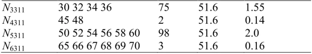
Set Ndkjl Operations of Ndkjl L(Ndkjl) γdkjl tb(Pdkjl) N1121 9 11 13 15 24 83.6 0.39 N2121 26 2 62.7 0.13 N3121 37 39 41 43 24 83.6 0.39 N1122 10 14 18 20 25 82.2 0.4 N2122 27 2 62.7 0.13 N3122 38 42 9 106.3 0.18 N1123 12 16 17 19 25 82.2 0.4 N2123 28 2 62.7 0.13 N3123 40 44 9 106.3 0.18 N2124 25 2 62.7 0.13 N1211 1 3 5 7 79 51.6 1.63 N2211 22 23 2 51.6 0.14 N3211 29 31 33 35 79 51.6 1.63 N4211 46 47 2 51.6 0.14 N5211 49 51 53 55 57 59 100 51.6 2.04 N6221 61 40 74.1 0.64 N6222 62 24 197.1 0.22 N6223 63 24 161.6 0.25 N6224 64 18 160.2 0.21 N1311 2 4 6 8 75 51.6 1.55 N2311 21 24 2 51.6 0.14
N3311 30 32 34 36 75 51.6 1.55
N4311 45 48 2 51.6 0.14
N5311 50 52 54 56 58 60 98 51.6 2.0
N6311 65 66 67 68 69 70 3 51.6 0.16
Table 10. Characteristics of the optimal solution
Position p tp(P1k) tp(P2k) tp(P3k) tp(P4k) tp(P5k) tp(P6k)
1 1.79 1.02 1.25 0.1 0.1 0.1
2 1.73 0.24 1.73 0.24 2.14 1.92
3 1.65 0.24 1.65 0.24 2.1 0.26
Then, we solve problem (1) – (38) again with CPLEX 12.2 but by using the reduction of constraints (20) as explained in Section 2. The obtained optimal solution and its characteristics are presented in Tables 11 and 12. The number of variables in the model is 828 and the number of constraints is 4824. The solution time was 1.21. There is the vertical spindle head common for positions 2 and 3. Parts 1, 2, 3, 4, 5 are machined at the position 2, and all the parts are machined at the position 3. There are installed the horizontal turret with 4 machining modules (part 6; part 6; part 6; part 6) at the position 1 and the horizontal turret with 4 machining modules (part 2; parts 1, 2, 3; parts 1, 2, 3; parts 1, 2, 3) at the position 2. The rotary table turns 1.65 min after the start, then in 2.14 min, 2.1 min, 1.73 min, 1.65 min, 1.92 min, 0.1 min, and in 1.73 min, respectively. The total time for machining all parts of the batch is 13.02 min. Table 11. An optimal solution
Set Ndkjl Operations of Ndkjl L(Ndkjl) γdkjl tb(Pdkjl) N6121 61 40 74.1 0.64 N6122 62 24 197.1 0.22 N6123 63 24 161.6 0.25 N6124 64 18 160.2 0.21 N1211 1 3 5 7 79 51.6 1.63 N2211 22 23 2 51.6 0.14 N3211 29 31 33 35 79 51.6 1.63 N4211 46 47 2 51.6 0.14 N5211 49 51 53 55 59 57 100 51.6 2.04 N2221 28 2 62.7 0.13 N1222 9 11 13 15 24 83.6 0.39 N2222 26 2 62.7 0.13 N3222 37 39 41 43 24 83.6 0.39 N1223 12 16 17 19 25 82.2 0.4 N2223 25 2 62.7 0.13 N3223 40 44 9 106.3 0.18 N1224 10 14 18 20 25 82.2 0.4 N2224 27 2 62.7 0.13 N3224 38 42 9 106.3 0.18 N1311 2 4 6 8 75 51.6 1.55 N2311 21 24 2 51.6 0.14 N3311 30 32 34 36 75 51.6 1.55 N4311 45 48 2 51.6 0.14 N5311 50 52 54 56 60 58 98 51.6 2.0 N6311 65 66 67 68 69 70 3 51.6 0.16
Table 12. Characteristics of the optimal solution
Position k tp(P1k) tp(P2k) tp(P3k) tp(P4k) tp(P5k) tp(P6k)
1 0.1 0.1 0.1 0.1 0.1 1.92
2 1.73 1.02 1.73 0.24 2.14 0.1
3 1.65 0.24 1.65 0.24 2.1 0.26
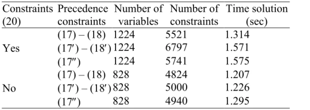
Finally, the summary of the generated models and obtained results for different combinations of constraints (20), (17) – (18), (17) – (18), and (17) is presented in Table 13.
Table 13. Characteristics of the models Constraints (20) Precedence constraints Number of variables Number of constraints Time solution (sec) Yes (17) – (18) 1224 5521 1.314 (17) – (18) 1224 6797 1.571 (17) 1224 5741 1.575 No (17) – (18) 828 4824 1.207 (17) – (18) 828 5000 1.226 (17) 828 4940 1.295
The locations of parts at the loading position and the general view of the designed rotary transfer machine according to the solution from Table 9 are presented in Fig. 2 and Fig. 3.
5. EXPERIMENTAL STUDY
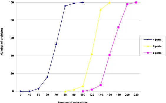
The purpose of this study is to evaluate the effectiveness of the proposed optimization approach. Series of 100 test instances for 4, 6 and 8 different parts were generated. Their characteristics are presented in Fig. 10-11 and Tables 14-16, where |N| is the number of operations, OSP is the order strength of precedence constraints, DM, DT, DP, SS, and SM are the densities of graphs GDM, GDT, GDP, GSS, and GSM , respectively. The constraints were generated using the techniques and software presented in (Dolgui et al, 2008). Experiments were carried out on ASUS notebook (1.86 Ghz, 4 Gb RAM) with academic version of CPLEX 12.2.
Fig. 10 Characteristics of test instances (number of operations)
Fig. 11 Characteristics of test instances (loading sequence length) Table 14 Test series with 4 parts
Parameters of problems |N| OSP DM DT DP SS SM LS
Minimal value 44 0.034 0.064 0.026 0 0.027 0 4 Maximal value 95 0.161 0.659 0.659 0.242 0.051 0.016 8 Average value 69 0.102 0.373 0.348 0.023 0.036 0.004 6 0 20 40 60 80 100 0 40 50 60 70 80 90 100 120 140 160 180 200 220 Numbe r of proble m s Number of operations 4 parts 6 parts 8 parts 0 20 40 60 80 100 0 2 4 6 8 9 10 12 Numbe r of proble m s
Length of loading sequence
4 parts
6 parts
Table 15 Test series with 6 parts
Parameters of problems |N| OSP DM DT DP SS SM LS
Minimal value 89 0.029 0.003 0.002 0 0.024 0 6
Maximal value 159 0.111 0.462 0.462 0.205 0.031 0.008 9
Average value 124 0.08 0.229 0.198 0.028 0.027 0.002 7
Table 16 Test series with 8 parts
Parameters of problems |N| OSP DM DT DP SS SM LS
Minimal value 118 0.023 0.004 0.004 0 0.024 0 8
Maximal value 216 0.083 0.526 0.525 0.214 0.033 0.006 12
Average value 166 0.055 0.297 0.266 0.027 0.028 0.002 10
First, we compare the results of using model (1) – (38) with different combinations of constraints (20), (17) – (18), (17) – (18), and (17) for test instances with 4 parts.
By analyzing the results presented in Table 17, we can see the positive impact of the reduction of constraints (20).
Table 17 Impact of the transformation of constraints (20) on test series with 4 parts
Parameters With inclusion
constraints (20)
With reducing inclusion constraints (20)
Minimal time (sec) 1.32 0.76
Maximal time (sec) 601.074 609.27
Average time (sec) 38.238 33.912
Total time (sec) 3823.81 3391.17
Number of instances solved in shorter time
86 14
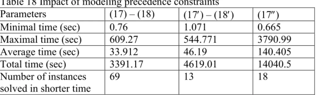
Then, we compare the effectiveness of modeling precedence constraints by (17) – (18), (17) – (18) and (17). The summary results are presented in Table 18.
Table 18 Impact of modeling precedence constraints
Parameters (17) – (18) (17) – (18) (17)
Minimal time (sec) 0.76 1.071 0.665
Maximal time (sec) 609.27 544.771 3790.99
Average time (sec) 33.912 46.19 140.405
Total time (sec) 3391.17 4619.01 14040.5
Number of instances solved in shorter time
69 13 18
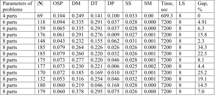
Finally, we present in Table 19 the summary results of solving 3 series of 100 test instances for 4, 6, and 8 parts with constraints (17) – (18) and the transformation of constraints (20). The maximal available time was set up to 2 hours (7200 sec). Feasible solutions were found for all test instances. However, only for 2 instances with 6 parts the optimality of found solutions was not proved while the number of such instances with 8 parts is equal to 11 with maximal gap 34.3 % (see Table 20). Number of solved problems in function of time is depicted in Figure 12. Parameters of easy and hard instances are presented in Table 20 and 21, respectively.
Table 19 Time solution of test instances
Parameters 4 parts 6 parts 8 parts
Minimal time (sec) 0.76 0.678 1.693
Maximal time (sec) 609.27 7200 7200
Average time (sec) 33.912 703.742 1767.59
Total time (sec) 3391.17 70374.2 174992
Number of solved instances
100 100 100
Number of instances with proven optimality
100 98 89
Table 20 Parameters of easy test instances Parameters of problems |N| OSP DM DT DP SS SM LS Time, sec 4 parts 63 0.093 0.598 0.591 0.001 0.037 0.002 4 0.76 6 parts 106 0.086 0.024 0.014 0.009 0.030 0.003 6 0.68 8 parts 159 0.065 0.162 0.161 0.000 0.024 0.000 8 1.69
Table 21 Parameters of hard test instances Parameters of problems |N| OSP DM DT DP SS SM Time, sec LS Gap, % 4 parts 69 0.104 0.249 0.141 0.100 0.033 0.00 609.3 8 0 6 parts 118 0.094 0.335 0.291 0.037 0.028 0.000 7200 8 4.91 6 parts 159 0.065 0.335 0.291 0.037 0.028 0.000 7200 8 6.3 8 parts 176 0.061 0.291 0.276 0.009 0.027 0.001 7200 8 15.8 8 parts 148 0.043 0.232 0.155 0.062 0.031 0.001 7200 8 2.3 8 parts 185 0.079 0.264 0.226 0.026 0.026 0.000 7200 8 34.3 8 parts 185 0.079 0.260 0.220 0.032 0.026 0.001 7200 8 22.5 8 parts 175 0.073 0.277 0.220 0.046 0.028 0.001 7200 8 8.1 8 parts 177 0.073 0.230 0.221 0.006 0.025 0.002 7200 8 4.4 8 parts 170 0.072 0.185 0.169 0.010 0.027 0.001 7200 8 25.2 8 parts 132 0.053 0.316 0.254 0.046 0.032 0.001 7200 8 19.1 8 parts 180 0.060 0.219 0.046 0.168 0.028 0.000 7200 8 14.5 8 parts 179 0.060 0.378 0.295 0.075 0.026 0.000 7200 8 7.0
Fig. 12 Time solution diagram
6. CONCLUSION
This paper has proposed a joint formulation for process planning and system configuration for design of rotary transfer machines for a mixed-model production of different parts. The objective of suggested models is to minimize the total system cost. A mathematical formulation with several variants for this combinatorial optimization problem was developed and evaluated on an industrial case study. It was shown that the developed models could be successfully applied to the production cases with 6 different types of parts to be machined simultaneously at such a transfer machine. However, since the problem size is substantially increasing when the number of different types of parts is growing, as a consequence, it makes difficult to obtain optimal solutions for larger problem sizes. To address such problems efficiently within reasonable solution time, approximate methods have to be developed. Having such methods available will also allow envisaging the extension of the optimization problem by considering the sequence of the parts to be determined at the same time as the process planning and the system configuration.
REFERENCES
Battaïa, O., Brissaud, D., Dolgui, A., Guschinsky, N. (2015) Variety-oriented design of rotary production systems. CIRP Annals - Manufacturing Technology, 64:1, 411-414.
Battaïa, O., Dolgui, A., Guschinsky, N., and Levin, G. (2014a). Combinatorial techniques to optimally customize an automated production line with rotary transfer and turrets. IIE Trasactions, 46 (9), 867-879. Battaïa, O., Dolgui, A., Guschinsky, N., Levin, G. (2014b) Integrated configurable equipment selection and line balancing for mass production with serial–parallel machining systems, Engineering Optimisation, 46:10, 1369-1388.
Battaïa, O., Dolgui, A., Guschinsky, N., and Levin, G. (2012a). A decision support system for design of mass production machining lines composed of stations with rotary or mobile table. Robotics and Computer-Integrated Manufacturing, 28, 672-680.
Battaïa, O., Dolgui, A., Guschinsky, N., and Levin, G. (2012b). Optimal design of machines processing pipeline parts. International Journal of Advanced Manufacturing Technology, 63, 963-973.
0 20 40 60 80 100 Number of problems
Time solution, sec
4 parts 6 parts 8 parts
Bensmaine, A., Dahane M., Benyoucef. L. (2014) A new heuristic for integrated process planning and scheduling in reconfigurable manufacturing systems, International Journal of Production Research, 52:12, 3583-3594.
Chryssolouris, G., Chan, S., Suh, N.P. (1985) An integrated approach to process planning and scheduling, CIRP Annals-Manufacturing Technology, 34:1, 413–417.
Copani, G., Leonesio, M., Molinari Tosatti, L., Pellegrinelli, S., Urgo, M., Valente, A. (2015) An integrated framework for combined designing dematerialised machine tools and production systems enabling flexibility-oriented business models, International Journal of Computer Integrated Manufacturing, 28:4, 353-363.
Copani, G., Rosa, P. (2015) DEMAT: sustainability assessment of new flexibility-oriented business models in the machine tools industry, International Journal of Computer Integrated Manufacturing, 28:4, 408-417.
Dolgui, A., Guschinsky, N., Levin, G. Proth, J.M. (2008) Optimisation of multi-position machines and transfer lines, European Journal of Operational Research, 185:3, 1375-1389.
Dolgui, A., Guschinsky, N., Levin, G. (2009) Graph approach for optimal design of transfer machine with rotary table, International Journal of Production Research, 47:2, 321–341.
Guschinskaya, O., Dolgui, A., Guschinsky, N., and Levin, G. (2009). Minimizing makespan for multi-spindle head machines with a mobile table. Computers and Operations Research, 36 (2), 344–357.
Leonesio, M., Molinari Tosatti, L., Pellegrinelli, S., Valente, A. (2013) An integrated approach to support the joint design of machine tools and process planning. CIRP Journal of Manufacturing Science and Technology, 6, 181–186.
Li, W. D., McMahon, C. A. (2007) A simulated annealing-based optimization approach for integrated process planning and scheduling, International Journal of Computer Integrated Manufacturing, 20:1, 80-95.
Lv, S., Qiao, L. (2014) Process planning and scheduling integration with optimal rescheduling strategies, International Journal of Computer Integrated Manufacturing, 27:7, 638-655.
Makssoud, F., O. Battaïa, A. Dolgui. An exact optimization approach for a Transfer Line Reconfiguration Problem. International Journal of Advanced Manufacturing Technology, 72 (2014) 717-727.
Mohapatra, P., Kumar, N., Matta, A., Tiwari, M.K. (2014) A nested partitioning-based approach to integrate process planning and scheduling in flexible manufacturing environment, International Journal of Computer Integrated Manufacturing, DOI: 10.1080/0951192X.2014.961548
Phanden R. K., Jain, A., Verma, R. (2011) Integration of process planning and scheduling: a state-of-the-art review, International Journal of Computer Integrated Manufacturing, 24:6, 517-534.
Phanden R. K., Jain, A., Verma, R (2013) An approach for integration of process planning and scheduling, International Journal of Computer Integrated Manufacturing, 26:4, 284-302.
Rabbani, M., Ziaeifar A., Manavizadeh N. (2014) Mixed-model assembly line balancing in assemble-to-order environment with considering express parallel line: problem definition and solution procedure, International Journal of Computer Integrated Manufacturing, 27:7, 690-706.
Szadkowski J. (1971) An approach to machining process optimization, International Journal of Production Research, 9:3, 371-376.
Terkaj, W., Tolio, T., Valente, A. (2010) A stochastic programming approach to support the machine tool builder in designing focused flexibility manufacturing systems (ffmss), International Journal of Manufacturing Research, 5, 199-229.
Terkaj, W., Tolio, T., Valente, A. Focused flexibility in production systems, H. ElMaraghy (Ed.), Changeable and reconfigurable manufacturing systems, Springer, Berlin (2009), pp. 47-66.
Tolio, T., Urgo, M., (2013) Design of flexible transfer lines: A case-based reconfiguration cost assessment, Journal of Manufacturing Systems, 32:2, 325-334.
Xu, X., Wang, L., Newman S.T. (2011) Computer-aided process planning – A critical review of recent developments and future trends, International Journal of Computer Integrated Manufacturing, 24:1, 1–31. Yin, R., Cao, H., Li H., Sutherland J.W. (2014) A process planning method for reduced carbon emissions, International Journal of Computer Integrated Manufacturing, 27:12, 1175-1186.