Automated multimodal volume registration based on supervised 3D anatomical landmark detection

Automated multimodal volume registration based on supervised 3D

anatomical landmark detection

R´emy Vandaele

1

, Franc¸ois Lallemand

2

, Philippe Martinive

2

, Akos Gulyban

2

, S´ebastien Jodogne

2,3

,

Philippe Coucke

2

_{, Pierre Geurts}

1

_{, Rapha¨el Mar´ee}

1

1_{Montefiore Institute, University of Li`ege, Grande Traverse 10, Li`ege, Belgium} 2_{Department of Radiotherapy and Oncology, University of Li`ege, Li`ege, Belgium}

3_{Department of Medical Physics, University of Li`ege, Li`ege, Belgium} {remy.vandaele, raphael.maree}@ulg.ac.be

Keywords: Registration, Machine Learning, Oncology Applications, Radiation Therapy, Urology and Pelvic Organs, Computed Tomography

Abstract: We propose a new method for automatic 3D multimodal registration based on anatomical landmark detection. Landmark detectors are learned independantly in the two imaging modalities using Extremely Randomized Trees and multi-resolution voxel windows. A least-squares fitting algorithm is then used for rigid registration based on the landmark positions as predicted by these detectors in the two imaging modalities. Experiments are carried out with this method on a dataset of pelvis CT and CBCT scans related to 45 patients. On this dataset, our fully automatic approach yields results very competitive with respect to a manually assisted state-of-the-art rigid registration algorithm.

1

INTRODUCTION

In radiotherapy, the 3D Computed Tomography Scan-ner (CT-Scan) is used as the reference for treatment dosimetry and patient positioning. During the treat-ment itself, a Cone-Beam-CT-Scan (CBCT) is ac-quired several times at the treatment machine to en-sure the proper positioning of the patient with respect to the simulation CT-Scan so as to correctly deliver the treatment to the tumor. Registration of the two modalities are thus needed in routine applications. Usually, the registration is performed semi-manually by a human operator.

The problem of multimodal rigid volume registra-tion consists in finding the deformaregistra-tion (translaregistra-tions and rotations) that will minimize the difference be-tween the two images or volumes to register. This dif-ference can be evaluated using several possible met-rics such as voxel by voxel mutual information or normalized correlation, but also, as in this paper, us-ing the distance between common specific landmarks identified in both volumes. Several general optimiza-tion algorithms have been proposed for multimodal

This is the author’s final version of VISAPP 2017 accepted paper to be published by SCITEPRESS (http://www.visapp.visigrapp.org/)

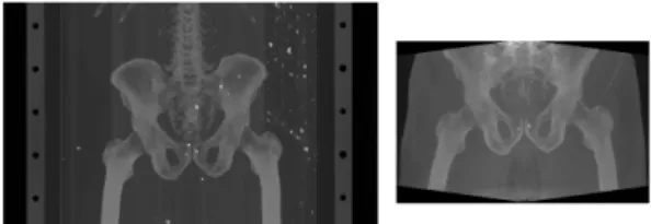
Figure 1: Sample volumes (MIP projections) from our dataset. On the left, a CT scan, on the right, a CBCT scan. Notice the differences between the scanned body regions.

rigid registration (Zitova and Flusser, 2003),(Pluim et al., 2003). However, because the scanned regions can differ between the two volumes to register, these algorithms do not perform well enough without man-ual intervention for medical registration: an operator is required to manually define in the two images the region of interest (ROI) in which the registration pro-cedure should be applied (Hill et al., 2001). For exam-ple, as shown in Figure 1 for CT-CBCT registration in radiotherapy, CT images will typically correspond to large body scans, while CBCT images will corre-spond to specific parts of the body (e.g. organs). The application of out-of-the-box registration algorithms such as 3D-Slicer (Fedorov et al., 2012) or Elastix (Klein et al., 2010) on the whole CT and CBCT im-ages will thus fail as it will try to register the full body

in CT to a specific organ in CBCT. The ROI for the registration therefore needs to be manually selected in both images, which significantly slows down the registration process.

In this paper, we propose, and evaluate, a novel fully automated (i.e., free from any manual ROI selec-tion) multimodal rigid volume registration algorithm. The main idea of this approach is to first automati-cally detect several 3D anatomical landmarks in each image modality, using supervised machine learning techniques, and then to register the two images only on the basis of these landmarks. Our hypothesis is that although patients have different appearances, a specific anatomical landmark is likely to look very similar among different patients in a given imaging modality, hence each landmark appearance could be learned in each modality. We want therefore to eval-uate such an approach where anatomical landmarks are detected independantly in each modality using su-pervised learning, then registered, in contrast to com-monly used approaches that rely on the design and matching of invariant features accross modalities.

In Section 2, we present our 3D landmark detec-tion method and explain how it is exploited for rigid registration. In Section 3, we introduce our dataset of simulation-CT and CBCT and summarize our land-mark detection and registration results. Finally, we conclude in Section 4.

2

METHOD

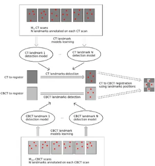
In our approach, landmark detection models are built for each landmark and each modality independently using training images and expert ground-truth land-mark positions. If N landmarks have to be de-tected, 2N detection models will be built (one for each landmark and each modality). For new volumes, once the landmarks are detected automatically in each modality, the registration is then performed through a matching point registration algorithm (Arun et al., 1987) using all the detected landmark position pairs. A graphical representation of our approach is given in Figure 2.

In this section, we first describe the learning ap-proach we used for the landmark detection, and then the registration method we used in order to perform the multimodal volume registration.

2.1

Supervised 3D Landmark Detection

Local, learning-based, feature detectors are promis-ing approaches for landmark detection in 2D and 3D

Figure 2: Representation of our CT-to-CBCT registration algorithm.

images. They have been shown recently to outper-form global landmark matching algorithms in various applications (Fanelli et al., 2013; Wang et al., 2015). Here, we extended the 2D landmark detection method of (Stern et al., 2011) to 3D imaging.

Our algorithm is based on supervised learning: manually annotated volumes are used to train models (Extremely Randomized Trees (Geurts et al., 2006)) able to predict the landmark positions in new vol-umes. As in (Stern et al., 2011), we propose and compare two approaches: in the first, a classifica-tion model is trained for each landmark to predict if a voxel corresponds to the landmark position. In the second, a regression model is trained to predict the euclidean distance between a voxel and the landmark position.

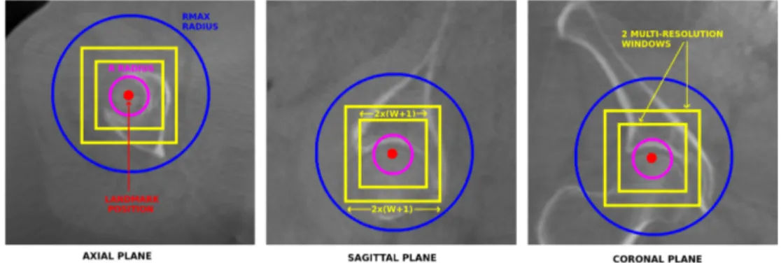
Voxel Description. Each voxel v in the training sample is described by D multi-resolution square voxel windows of side size 2W + 1 centered on v on each of the three axes. W and D are method pa-rameters. It means that one voxel is described by 3D((2W + 1)2) features. In order to manage possi-ble luminosity variations, the volume voxel values are normalized and the feature values are computed as the difference between each voxel value and the value of the voxel v. Parameters W and D are illustrated in Figure 3.

Classification Output. We consider a binary voxel classification model. The voxels can either belong to

Figure 3: Illustration of the different parameters for one landmark in a CBCT scan. The multi-resolution windows describe the landmark voxel.

the landmark class (1) or to the non landmark class (-1). Only one position in each image corresponds to the landmark. If only these positions are consid-ered as landmarks, and if N training images are avail-able, only N positive examples will be available to train our voxel classification model. To extend the set of positive examples, we consider as positive ex-amples all voxels that are at a distance at most R from the landmark, where R is a method parameter illustrated in Figure 3. If the landmark is at posi-tion (xl, yl, zl) in an image, then the output class of a pixel at position (x, y, z) in the same image will be 1 if (x − x_l)2_{+ (y − y}

l)2+ (z − zl)2≤ R2, or −1 otherwise.

Regression Output. With the regression method, the output associated to each voxel is the euclidean distance between this voxel and the landmark position in the training image. More formally, if the landmark is at position (xl, yl, zl) in an image, then the output value of a pixel at position (x, y, z) in the same image will bep(x − xl)2+ (y − yl)2+ (z − zl)2

Voxel Sampling Scheme. In both cases, the clas-sification or the regression model is trained from a learning sample composed of all the4₃πR3voxels that are located within a distance d ≤ R to the landmark position (the landmark class with the classification approach) and P4₃πR3 voxels located at random po-sitions within a distance R < d ≤ Rmax to the land-mark position (the non-landland-mark class for the classi-fication approach), where P and Rmaxare user defined parameter. R and Rmax are represented in Figure 3. In classification, sampling all the pixels inside the R radius allows us to sample more landmark voxels in the positive class than uniform sampling. For the re-gression approach, this parameter allows us to sam-ple more voxels close to the real landmark position, which helps the model to perform a better differen-tiation for the voxels close to the landmark position.

On the other hand, the effect of the Rmax parameter is to artificially reduce the number of distant voxels, which allows to reduce the size of the dataset, while having little to no effect on the prediction accuracy, as we will show in our experiments.

Model Training. The voxel classification or regres-sion model is trained using the Extremely Random-ized Trees algorithm (Geurts et al., 2006). This learn-ing algorithm is a variant of the Random Forest al-gorithm (Breiman, 2001) offering similar accuracy than regular Random Forest while speeding up model training. In this algorithm, an ensemble of T decision or regression trees are built from the original train-ing sample (no bootstraptrain-ing), without pruntrain-ing. At each node, the best split is selected among K features chosen at random, where K is a number between 1 and the total number of features. For each of the K (continuous) selected features, a separation threshold is chosen at random within the range of the feature in the subset of the observations (i.e., voxels) in the node. A score is computed for each pair of feature and threshold, and the best pair according to a score measure is chosen. We chose to use the Gini index reduction score for classification, and the variance re-duction score for our regression trees.

Landmark prediction. During the radiotherapy process, the patients are placed in the same position according to the tumor location. When considering specific tumor locations, the landmarks will be found in close areas from one image to another. In con-sequence, it would be inefficient to search for each landmark in the whole volume. This is why instead of thoroughly scanning the volume, we are consider-ing another solution: in a new volume, we extract Np voxels taken at random locations following the nor-mal distribution

_N

(¯µ, Σ2_{), where ¯µ is the mean} po-sition of the landmark in the training dataset, and Σ

the corresponding covariance matrix. The predicted position of the landmark in a new volume will either be the median of the locations of the voxels predicted as landmarks with the highest probability (classifica-tion), or as the closest to the landmark position (re-gression).

Parameter setting. The method depends on several parameters: the radius R and Rmax, the ration of non-landmark versus non-landmark voxels P, the number of voxels Npto extract for computing a prediction, the number of trees T , the size of the window W and the number of resolutions D. These parameters are either set to their maximum value given the avail-able computing resources (T, Np) or tuned through cross-validation. Trees were fully grown (nmin= 2) and the K parameter was set to its default value p

3D((2W + 1)2_{) (Geurts et al., 2006).}

2.2

Multimodal Landmark-based Rigid

Registration

Once anatomical landmark coordinates have been predicted in both images, the registration of the re-sulting matching pairs of landmark positions is for-mulated as the least-square optimization problem pre-sented in (1). min X,T N

∑

i=1 ||p0_i− (X pi+ T )||2 (1) Nis the number of landmarks, piand p0i are the co-ordinates of the ith landmark in the two images, X is a 3 × 3 rotation matrix, and T a 3 × 1 translation vector. To solve this problem, we use the noniterative SVD-based algorithm proposed in (Arun et al., 1987). It is important to notice that, as opposed to volume registration based on local feature detectors and in-variant descriptors (e.g. (Lukashevich et al., 2011)), our method does not require matching of landmark descriptors accross modalities.

3

EXPERIMENTS AND RESULTS

In this section, we first describe our dataset, divided into a training and a test set. Then, we study system-atically the influence of the main parameters of our landmark detection method by leave-one-patient-out validation on the training set. Finally, we present reg-istration results on the test set and compare them to a semi-automated volume registration algorithm (Fe-dorov et al., 2012).

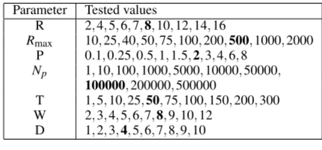
Table 1: Sets of values tested during cross-validation for each parameter. In bold, the default value of each parameter used in the first stage of cross-validation.

Parameter Tested values

R 2, 4, 5, 6, 7, 8, 10, 12, 14, 16 Rmax 10, 25, 40, 50, 75, 100, 200, 500, 1000, 2000 P 0.1, 0.25, 0.5, 1, 1.5, 2, 3, 4, 6, 8 Np 1, 10, 100, 1000, 5000, 10000, 50000, 100000, 200000, 500000 T 1, 5, 10, 25, 50, 75, 100, 150, 200, 300 W 2, 3, 4, 5, 6, 7, 8, 9, 10, 12 D 1, 2, 3, 4, 5, 6, 7, 8, 9, 10

3.1

Datasets

Our dataset contains images related to 45 patients (male and female) and was acquired at the Radiother-apy and Oncology Department, University of Li`ege, Belgium. For each of these patients, we have one pelvic CT scan as the reference (45 CTs in total), and at least one corresponding CBCT scan of the pelvis (68 CBCTs in total). We divided this dataset into a training set of 30 patients, each with one CT and at least one CBCT (i.e 53 CBCTs in total), and a test set of 15 patients, each with exactly one CT and one CBCT.

Because our algorithm works better with volumes of identical resolutions and the original resolution information is always available, each CT and each CBCT were resized to 1 × 1 × 1mm voxel resolution. Originally, CT scan resolutions were comprised be-tween 0.5 and 3mm. The CBCT scans were acquired with an Elekta XVI scanner, that were reconstructed to 1 × 1 × 1mm resolution. More information about the quality of the CBCT image acquisition procedure can be found in (Kamath et al., 2011).

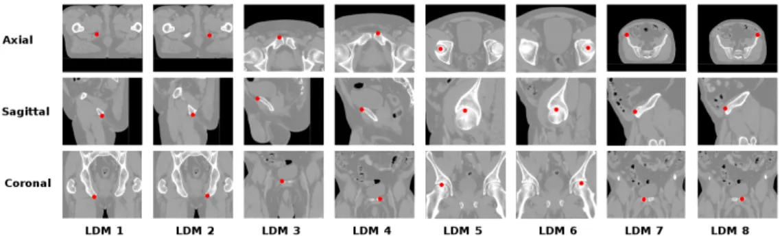
On each CT and each CBCT, 8 landmarks dis-tributed in the pelvis were manually annotated two times by the same skilled operator. The mean distance between the two annotation runs is shown in Table 2 (Manual Err.). The position of each landmark is pre-sented in Figure 4 for CT scans. We used as ground-truth for each landmark the mean coordinates of the two manual annotations provided by the operator.

3.2

Landmark Detection Results

3.2.1 Protocol

For our experiments, we fixed extremely random-ized tree parameters to recommended values (K = p

3D((2W + 1)2_{), n}

min = 2) (Geurts et al., 2006). Other parameter values were evaluated in the ranges presented in Table 1.

Figure 4: Representative pictures showing the position of the 8 landmarks on a CT-scan.

These values were tested for both the regression and the classification approaches using leave-one-patient-out in the training set. Since it is not possible to explore all parameter combinations, we use a two-stage approach. In the first two-stage, for each parameter in turn, all its values were tested with the other pa-rameters set to some default value (in bold in Table1). In the second stage, the exact same procedure was ap-plied by using as a new default value for each param-eter the value that led to the lowest CV error (in aver-age over all landmarks) in the first staver-age. The best val-ues for each parameter in this second round were then identified, this time for each landmark separately, and used to retrain a model using all training images. In total, 4480 parameter combinations were tested using computer clusters.

3.2.2 Influence of Method Parameters

The influence of method parameters is shown in Fig-ure 5. We did not notice major differences between the classification and the regression approaches. For some particular landmarks, the performance was worse for the CBCT scans. We believe that this differ-ence is mainly due to one particular patient for which our algorithm had difficulties because of its particular CBCT localization: the regions containing the land-marks 3, 4, 7 and 8 was not acquired. For the classifi-cation approach, the R parameter clearly needs to be tuned: too small R will lead to too few positive ex-amples in the dataset, while too large R will associate too distant voxels to the positive class. The regres-sion approach is less sensitive to too large R values. We noticed that small values of Rmax(25-40 voxels) work better for both classification and regression. We explain that by the fact that the landmark structure is unique inside the volume, and thus learning to dis-criminate close voxels is more effective than com-paring more distant voxels. Increasing the propor-tion P improves the performance for classificapropor-tion but smaller P values can be used for regression (which de-creases the size of the dataset). Increasing the number

Figure 5: Influence of method parameters From top to bot-tom, left to right: R, Rmax, P, Np, T,W, D. The y−axis is the CV error (in mm) averaged over all landmarks.

.

of predictions Npalways improves the performance as expected. However, optimal performance is already attained with Np= 100000. The same effect is ob-served with the number of trees T , with optimal per-formance reached at T = 50. The windows size W controls the number of features and the locality of the information that is provided for each voxel. This pa-rameter clearly needs to be tuned with values in the range 6–8 being optimal in most cases. Increasing the number of resolutions D quickly increases the error,

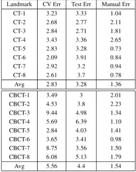
Table 2: Test set results (error in mm). Landmark CV Err Test Err Manual Err

CT-1 3.23 3.33 1.04 CT-2 2.68 2.77 2.11 CT-3 2.84 2.71 1.81 CT-4 3.43 3.36 2.65 CT-5 2.83 3.28 0.73 CT-6 2.09 3.91 0.84 CT-7 2.92 3.2 0.94 CT-8 2.61 3.7 0.78 Avg 2.83 3.28 1.36 CBCT-1 3.49 3 2.01 CBCT-2 4.53 3.8 2.23 CBCT-3 9.44 4.98 1.34 CBCT-4 5.69 6.39 1.10 CBCT-5 2.84 4.03 1.41 CBCT-6 3.65 3.41 0.98 CBCT-7 8.75 3.56 1.50 CBCT-8 6.08 5.13 1.79 Avg 5.56 4.4 1.54

most likely because it leads to overfitting. Small val-ues of D ' 2–3 are optimal in most cases.

3.2.3 Test Set Errors

Table 2 reports for each landmark the error obtained on the test set (column ’Test Err’) using the optimal parameter setting determined with the two-stage CV explained above. For comparison, columns ’CV Err’ and ’Manual Err’ provide respectively the optimal CV error on the training set and the error between the two manual annotations of the human operator.

Results are satisfactory although the difference between the algorithmic and the manual errors remain important. When interpreting these results, we have to take into account the low resolution of the CT and CBCT images that forced us to resize our voxels to a 1 × 1 × 1mm resolution. Given this resizing, an error of only 2 or 3 voxels directly translates into an error of 2 or 3mm. With CBCT scans of higher resolution, we could have resized the images to a higher common resolution, which should have led to a lower global error (in mm). Performance on the CBCT scans are worse than on the CT scans. We attribute this dif-ference to poorer image acquisition quality (Kamath et al., 2011).

3.3

Multimodal Volume Registration

Results

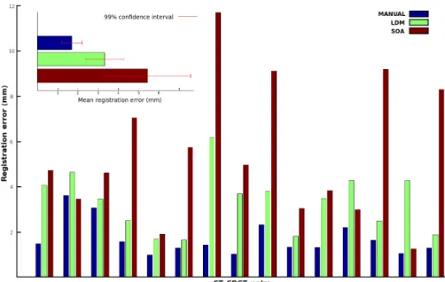
The registration results on all 15 CT-CBCT pairs in the test set are shown in Figure 6. The quality of the registration is measured by the average distance be-tween the ground-truth positions of the landmarks in the two images after their registration. LDM stands

for landmark registration. It corresponds to the pro-posed approach, i.e., the application of the registra-tion algorithm of (Arun et al., 1987) after the 8 pairs of landmarks were automatically detected in the CT and CBCT images using our algorithm. MANUAL corresponds to the application of the same registration algorithm but using the exact ground-truth positions of the landmarks. Its error is thus a lower bound on the error we can expect to achieve with our method. For comparison, we also provide the error obtained using the state-of-art (SOA) semi-automatic registra-tion method implemented in 3D-slicer (Fedorov et al., 2012) and described in (Johnson et al., 2007). We ap-plied the method within the smallest box-sized ROI surrounding all landmark positions and using the Mat-tes mutual information, which we found to be the best cost metric to use when compared to mean squared er-ror and normalized correlation.

As shown in Figure 6, the performance of SOA is unstable compared to our method and with respect to manual ground truths. For most patients, our al-gorithm performs much better. Globally, our results are very good. They show that our fully automatic approach performs better than (Johnson et al., 2007) which in addition requires a manual intervention for the delineation of the ROIs. The manual ground truth approach is most of the time much better than our ap-proach, suggesting that improving the quality of the landmark detectors, e.g. by collecting more train-ing images, could potentially improve even further the performance of our method.

On a Ubuntu 15.04 8 × 2.4Ghz, our paralellized python implementation of our algorithm takes 4 sec-onds for the complete registration (T = 50, D = 3, Np = 100000). We only take into account the CBCT landmark detection and the volume registra-tion, given that in radiotherapy practice, CT land-marks can be detected offline. On the same computer, the registration of the box-sized ROI of the CT and CBCT took approximately 7 seconds using 3D Slicer, which is also parallelized (Johnson et al., 2007).

4

CONCLUSION

In this work, we proposed a simple but efficient method for fully automated 3D multimodal rigid reg-istration based on automated anatomical landmark de-tection using supervised machine learning. We ap-plied our approach for pelvis CT-CBCT registration for patient positioning in radiotherapy. Our results showed that our automated approach is competitive with current state-of-art registration algorithms that require manual assistance. Given any kind of body

Figure 6: CT to CBCT registration results on the test set of 15 CT-CBCT pairs.

location and modality, interesting landmarks to regis-ter can be selected and detected by experts on a small training dataset, and then multi modal registration can be performed on new volumes by using our algorithm. In future works, we would like to manage the possi-bility to have landmarks out of the volume(s). Fu-ture works will also focus on non-rigid registration, where a higher number of landmarks will most prob-ably be required in order to perform plausible regis-trations. To specifically address this issue, another in-teresting future research direction would be to design techniques for the automatic selection of the most ap-propriate landmarks given pre-registered data. Be-yond this specific application, we also think that our 3D landmark detection method could be interesting in other areas such as morphometrics (Aneja et al., 2015).

ACKNOWLEDGEMENTS

R.V. was supported by F.N.R.S T´el´evie grant, R.M by research grant n1318185 of the Wallonia (DGO6). The authors thank the GIGA and the SEGI for provid-ing computprovid-ing resources as well as the Consortium des ´Equipements de Calcul Intensif (C ´ECI), funded by the Fonds de la Recherche Scientifique de Bel-gique (F.R.S.-FNRS) under Grant No. 2.5020.1.

REFERENCES

Aneja, D., Vora, S. R., Camci, E. D., Shapiro, L. G., and Cox, T. C. (2015). Automated detection of 3d land-marks for the elimination of non-biological variation in geometric morphometric analyses. In IEEE 28th International Symposium on Computer-Based Medi-cal Systems, pages 78–83. IEEE.

Arun, K. S., Huang, T. S., and Blostein, S. D. (1987). Least-squares fitting of two 3-d point sets. IEEE Trans-actions on pattern analysis and machine intelligence, (5):698–700.

Breiman, L. (2001). Random forests. Machine Learning, 45(1):5–32.

Fanelli, G., Dantone, M., Gall, J., Fossati, A., and Van Gool, L. (2013). Random forests for real time 3d face analysis. International Journal of Computer Vision, 101(3):437–458.

Fedorov, A., Beichel, R., Kalpathy-Cramer, J., Finet, J., Fillion-Robin, J.-C., Pujol, S., Bauer, C., Jennings, D., Fennessy, F., Sonka, M., et al. (2012). 3d slicer as an image computing platform for the quantita-tive imaging network. Magnetic resonance imaging, 30(9):1323–1341.

Geurts, P., Ernst, D., and Wehenkel, L. (2006). Extremely randomized trees. Machine learning, 63(1):3–42. Hill, D. L., Batchelor, P. G., Holden, M., and Hawkes,

D. J. (2001). Medical image registration. Physics in medicine and biology, 46(3):R1.

Johnson, H., Harris, G., Williams, K., et al. (2007). Brains-fit: mutual information rigid registrations of whole-brain 3d images, using the insight toolkit. Insight J, pages 1–10.

Kamath, S., Song, W., Chvetsov, A., Ozawa, S., Lu, H., Samant, S., Liu, C., Li, J. G., and Palta, J. R. (2011). An image quality comparison study between xvi and

obi cbct systems. Journal of Applied Clinical Medical Physics, 12(2).

Klein, S., Staring, M., Murphy, K., Viergever, M. A., and Pluim, J. P. (2010). Elastix: a toolbox for intensity-based medical image registration. IEEE Transactions on Medical Imaging, 29(1):196–205.

Lukashevich, P., Zalesky, B., and Ablameyko, S. (2011). Medical image registration based on surf detector. Pattern Recognition and Image Analysis, 21(3):519– 521.

Pluim, J. P., Maintz, J. A., and Viergever, M. A. (2003). Mutual-information-based registration of medical im-ages: a survey. IEEE Transactions on medical imag-ing, 22(8):986–1004.

Stern, O., Mar´ee, R., Aceto, J., Jeanray, N., Muller, M., Wehenkel, L., and Geurts, P. (2011). Automatic lo-calization of interest points in zebrafish images with tree-based methods. In IAPR International Confer-ence on Pattern Recognition in Bioinformatics, pages 179–190. Springer.

Wang, C.-W., Huang, C.-T., Hsieh, M.-C., Li, C.-H., Chang, S.-W., Li, W.-C., Vandaele, R., Mar´ee, R., Jodogne, S., Geurts, P., et al. (2015). Evaluation and com-parison of anatomical landmark detection methods for cephalometric x-ray images: a grand challenge. IEEE Transactions on medical imaging, 34(9):1890–1900. Zitova, B. and Flusser, J. (2003). Image registration

methods: a survey. Image and vision computing, 21(11):977–1000.