Carbon cycle dynamics during recent interglacials

(1)

CPD

11, 1945–1983, 2015 Carbon cycle dynamics during recent interglacials T. Kleinen et al. Title Page Abstract Introduction Conclusions References Tables Figures J I J I Back Close

Full Screen / Esc

Printer-friendly Version Interactive Discussion Discussion P a per | Discussion P a per | Discussion P a per | Discussion P a per |

Clim. Past Discuss., 11, 1945–1983, 2015 www.clim-past-discuss.net/11/1945/2015/ doi:10.5194/cpd-11-1945-2015

This discussion paper is/has been under review for the journal Climate of the Past (CP). Please refer to the corresponding final paper in CP if available.

Carbon cycle dynamics during recent

interglacials

T. Kleinen1, V. Brovkin1, and G. Munhoven2 1

Max Planck Institute for Meteorology, Bundesstr. 53, 20146 Hamburg, Germany

2

LPAP, Institut d’Astrophysique et de Géophysique, Université de Liège, Liège, Belgium Received: 22 April 2015 – Accepted: 29 April 2015 – Published: 20 May 2015

Correspondence to: T. Kleinen (thomas.kleinen@mpimet.mpg.de)

(2)

CPD

Full Screen / Esc

Printer-friendly Version Interactive Discussion Discussion P a per | Discussion P a per | Discussion P a per | Discussion P a per | Abstract

Trends in the atmospheric concentration of CO₂ during three recent interglacials, the Holocene, the Eemian and Marine Isotope Stage (MIS) 11, are investigated using an Earth system Model of Intermediate Complexity, which we extended with modules to dynamically determine two slow carbon cycle processes – peat accumulation and

5

shallow-water CaCO₃ sedimentation (coral reef formation). For all three interglacials, model simulations considering peat accumulation and shallow water CaCO₃ sedimen-tation substantially improve the agreement between model results and ice core CO₂ reconstructions in comparison to a carbon cycle setup neglecting these processes. This enables us to model the trends in atmospheric CO₂, with modelled trends similar

10

to the ice core data, forcing the model only with orbital and sea level changes. During the Holocene, anthropogenic CO₂emissions are required to match the observed rise in atmospheric CO₂ after 3 ka BP, but are not relevant before this time. Therefore our model experiments show for the first time how the CO₂evolution during the Holocene and two recent interglacials can be explained consistently using an identical model

15

setup.

1 Introduction

The atmospheric concentration of carbon dioxide (CO₂) increased from 260 to 280 ppm CO₂ during the Holocene between 8 ka BP and preindustrial. This trend in CO₂has to be seen in the context of previous interglacials, since all processes a

ffect-20

ing the atmospheric concentration, with the exception of possible human influences, should have been active during all interglacials. While the Holocene CO₂ trend has generated considerable interest previously (Ruddiman, 2003), the context of previous interglacials has been neglected. The present study aims to fill this gap.

Investigations of the Holocene trend in CO₂ can be classified into two basic

ap-25

(3)

CPD

Full Screen / Esc

approach. The inverse modelling approach takes the ice core record of CO₂ and

δ13CO₂as a starting point and aims to deduce the sources and sinks of CO₂from this record, while the forward modelling approach starts from the carbon cycle processes and aims to determine a CO₂trajectory from combinations of these.

Following the inverse modelling approach, based on records of CO₂ and its stable

5

carbon isotopic ratio δ13CO₂from ice cores, Indermühle et al. (1999) deconvolved the mass balance equations for CO₂and δ13CO₂to solve for the unknown terrestrial and oceanic sources and sinks of CO₂. They explained the changes in atmospheric CO₂ by major contributions from decreases in land carbon (C) storage and changes in sea surface temperature (SST), while changes in the cycling of CaCO₃played a minor role.

10

This approach was subsequently refined by Elsig et al. (2009) who presented new records of δ13CO₂ with higher resolution and precision. They explained the change in atmospheric CO₂ between 8 ka BP and preindustrial by carbonate compensation induced by earlier land-biosphere uptake, as well as coral reef formation, with some contribution by carbon release from the land biosphere.

15

Using the forward modelling approach, Ridgwell et al. (2003) used estimates of deep ocean carbonate ion concentrations to constrain the carbon cycle. They found that the observed trend in atmospheric CO₂during the last 8000 years can best be explained by the buildup of coral reefs and other forms of shallow water carbonate deposition. Joos et al. (2004), employing the Bern carbon cycle climate model to simulate the interval

20

from the last glacial maximum to preindustrial, found that a combination of processes contributed to the Holocene rise in CO₂, with carbonate compensation in response to terrestrial vegetation regrowth, SST changes and coral reef buildup playing a role. On the other hand, Brovkin et al. (2002), as well as Menviel and Joos (2012), found almost no effect of SST changes on CO₂during the Holocene.

25

Kleinen et al. (2010), using the CLIMBER2-LPJ model, showed that the trend in at-mospheric CO₂over the Holocene is controlled by the balance of two slow processes: carbon uptake by boreal peatlands, which is (slightly over)compensated by outgassing of CO₂due to sedimentation of CaCO₃ in shallow oceanic areas. Finally, Menviel and

(4)

CPD

Full Screen / Esc

Joos (2012) investigated the Holocene CO₂ rise by applying the Bern3D ocean car-bon cycle model, prescribing scenarios of shallow water carcar-bonate sedimentation and land C uptake. In their experiments, shallow water carbonate sedimentation, carbonate compensation of land uptake, land carbon uptake and release, and the response of the ocean-sediment system to marine changes during the termination contribute roughly

5

equally to the CO₂rise.

For earlier interglacials, investigations are rare. Schurgers et al. (2006) investigated the changes in atmospheric CO₂during both the Holocene and the Eemian using the GCM ECHAM3-LSG including the dynamic global vegetation model (DGVM) LPJ and the marine biogeochemistry model HAMOCC3. They found increases in atmospheric

10

CO₂for both Eemian and Holocene, mainly driven by decreases in terrestrial C storage, but they do not explain the overall magnitude of the CO₂ trend during the Holocene, and their positive trend in Eemian CO₂ is distinct from the ice core data, which shows no trend.

Here we address two major shortcomings of the study by Kleinen et al. (2010): (1)

15

both the accumulation of peatland carbon and the burial of CaCO₃ were prescribed and not modelled interactively, and (2) the study only considered the Holocene, while neglecting to show that the same mechanisms can also explain the evolution of CO₂ during previous interglacials. Our current model includes a dynamic peatland model, as well as a dynamic model of coral reef growth, which finally enables us to investigate

20

the evolution of atmospheric CO₂in interglacials previous to the Holocene. In this pa-per, we therefore aim to show how the evolution of CO₂ in three recent interglacials, the Holocene, the Eemian, and MIS 11, can be explained by the interplay of two slow carbon cycle processes, peat accumulation and CaCO₃ accumulation in shallow wa-ters.

(5)

CPD

Full Screen / Esc

2 Model and experiments 2.1 The model

To investigate these questions we are using CLIMBER2-LPJ, which consists of the Earth system Model of Intermediate Complexity (EMIC) CLIMBER2, coupled to the dy-namic global vegetation model (DGVM) LPJ. This combination of models allows

experi-5

ments on timescales of an interglacial due to the low computational cost of CLIMBER2, while accounting for the heterogeneity of land surface processes on the much finer grid of LPJ.

CLIMBER2 (Petoukhov et al., 2000; Ganopolski et al., 2001) consists of a 2.5-dimensional statistical-dynamical atmosphere with a latitudinal resolution of 10◦ and

10

a longitudinal resolution of roughly 51◦, an ocean model resolving three zonally av-eraged ocean basins with a latitudinal resolution of 2.5◦, a sea ice model, and a dy-namic terrestrial vegetation model (Brovkin et al., 2002). In the present model exper-iments, the latter model is used only for determining biogeophysical responses to cli-mate change, while biogeochemical effects, i. e., the corresponding carbon fluxes, are

15

determined by LPJ.

In addition CLIMBER2 contains an oceanic biogeochemistry model (Ganopolski et al., 1998; Brovkin et al., 2002, 2007) and a sediment model that describes the diffusive pore-water dynamics, assuming oxic only respiration and 4.5-order CaCO₃ dissolution kinetics (Archer, 1996; Brovkin et al., 2007). Volcanic emissions of CO₂are

20

assumed to be constant at 0.07 GtC a−1 (Gerlach, 2011). Weathering fluxes scale to runoff from the land surface grid cells, with separate carbonate and silicate lithologi-cal classes. The long-term carbon cycle that includes the processes of deep-sea and shallow-water carbonate accumulation, weathering and volcanic outgassing, is brought to equilibrium for the pre-industrial climate as in Brovkin et al. (2012).

25

We have coupled the DGVM LPJ (Sitch et al., 2003; Gerten et al., 2004) to CLIMBER-2 in order to investigate land surface processes at a resolution significantly higher than that of CLIMBER2. We also extended the model by implementing carbon

(6)

CPD

Full Screen / Esc

isotope fractionation according to Scholze et al. (2003). LPJ is run on a 0.5◦× 0.5◦grid and is called at the end of every model year simulated by CLIMBER2. Anomalies from the climatology of the temperature, precipitation and cloudiness fields are passed to LPJ, where they are added to background climate patterns based on the CRU-TS cli-mate data set (New et al., 2000). In order to retain some temporal variability in these

5

climate fields, the anomalies are not added to the climatology of the CRU-TS data set, but rather to the climate data for one year randomly drawn from the range 1901–1930. The change in the LPJ carbon pools is then passed back to CLIMBER2 as the car-bon flux F_ALbetween atmosphere and land surface and is employed to determine the atmospheric CO₂concentration for the next model year.

10

Biogeochemical feedbacks between atmosphere and land surface are thus deter-mined by the combination of CLIMBER2 and LPJ, while biogeophysical effects are solely determined by the CLIMBER2 land surface model, which includes its own dy-namical vegetation model. The latter model produces vegetation changes very similar to LPJ. Therefore discrepancies are very small.

15

2.2 Accumulation of Calcium carbonate in shallow waters

The accumulation of CaCO₃in shallow waters leads to an increase in the atmospheric CO₂ concentration. The production of CaCO₃ proceeds following the carbonate pre-cipitation equation Ca2++ 2HCO−₃ → CaCO₃+ CO2+ H2O. Under present conditions in seawater about 0.6 mol of CO₂ will be released for every mol of CaCO₃ produced

20

(Frankignoulle et al., 1994).

As part of the marine carbon cycle CLIMBER2 contains a model of early diagene-sis of carbonate in the deep sea sediments (Archer, 1996; Brovkin et al., 2007) and a model of carbonate accumulation in shallow waters derived from ReefHab (Kleypas, 1997). The original ReefHab predicts reef habitat area and accumulation of CaCO₃

25

in these environments as a function of temperature, salinity, nutrients, and light. The model considers corals as the main carbonate producers, but it is also applicable to calcareous algae, which have calcification rates very similar to corals.

(7)

CPD

Full Screen / Esc

For the implementation in CLIMBER2, we determined the potential reef area A by diagnosing the sea floor area above the maximum depth of reef growth for each ocean grid cell, depending on the global sea level, from the ETOPO2 data set (US Dept. of Commerce, 2006). In addition, we determined the topographic relief function TF, as de-scribed by Kleypas (1997). The vertical coral accumulation rate we then determine as

5

G= G_maxtanh(I_z/I_k), with G_maxthe maximum accumulation rate, I_z the Photosyntheti-cally Active Radiation (PAR) at depth z, and I_k the saturating light intensity necessary for photosynthesis. We calculate G for all grid cells where SST > 18.1 and < 31.5◦C, the growth limits for corals.

In the original Kleypas (1997) model, sea level is only used to calculate the area

10

available for shallow water sedimentation, but the rate of sea level change is not con-sidered in calculating the rate of CaCO₃ sedimentation. However, the rate of CaCO₃ accumulation by coral reefs will be strongly perturbed during periods of sea level drop or very fast sea level rise. A moderate rate of sea level rise, on the other hand, can maximise coral reef buildup. We therefore implemented a dependence of the CaCO₃

15

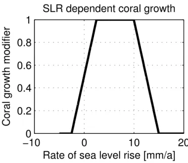
sedimentation rate on the rate of sea level change based on Munhoven and François (1996). Munhoven and François (1996) consider a trapezoidal growth-limiting function Θ as shown in Fig. 1, which restricts the coral reef growth in case sea-level rises too fast or falls. According to Buddemeier and Smith (1988) the best overall estimate for the sustained maximum rate of reef growth is 10 mm a−1. For simplicity we therefore adopt

20

0 and 10 mm a−1 as the limiting sea-level rates. To avoid too abrupt a change, accu-mulation rates are reduced from 100 to 0 % of the normal rate from 10 to 15 mm a−1; similarly we let them increase from 0 to 100 % from −2.5 mm a−1(i.e., a 2.5 mm a−1 de-crease) to+2.5 mma−1. We thus allow for a small accumulation even when sea-level falls. Carbonate accumulation rates will not drop to zero immediately since corals may

25

live even at depths of 50 m and more, and their habitat therefore does not vanish im-mediately.

The total CaCO₃production in each grid cell where ocean temperature is within the acceptable range therefore is P = G × Θ × A × T F , which we sum up for all grid cells

(8)

CPD

Full Screen / Esc

to determine the total shallow water CaCO₃ production. Total production is scaled to conform to the Milliman (1993) estimate of shallow water CaCO₃ sedimentation for the late Holocene. Milliman estimates a sedimentation rate in shallow waters of about 1.5 bt a−1(billion tons, Milliman’s units), which converts to 15 Tmol a−1using the CaCO₃ molar weight of 100 g mol−1.

5

The area factors A and TF are more or less constant over the sea level range of our experiments. Therefore variations in CaCO₃formation are primarily due to changes in the rate of sea level change. In experiments where the dynamic calculation of CaCO₃ sedimentation is disabled, a small constant shallow water CaCO₃sedimentation flux of 2 Tmol a−1is prescribed to balance the oceanic alkalinity budget.

10

2.3 Carbon accumulation in peatlands

According to Yu et al. (2010), global peatlands store about 615 Pg of carbon in the form of peat soils. The bulk of the carbon is contained in northern high latitude peat-lands, which contain about 550 Pg C, while tropical peatlands have accumulated about 50 Pg C and southern peatlands about 15 Pg C. This carbon was largely accumulated

15

since the last glacial maximum.

In order to account for this accumulation of carbon, we have extended the CLIMBER2-LPJ model by developing a dynamic model of peatland extent and peat carbon accumulation, as described in Kleinen et al. (2012). This model determines peatland extent from topography and climatic conditions. Within the peatland areas

20

obtained it considers the anoxic conditions in the soil to accumulate carbon in the mod-elled peatlands. For the last 8 ka, this model calculates an accumulation of 330 Pg C in high northern latitude areas, which is roughly in line with the Yu et al. (2010) estimate of 550 Pg C for the time period from the LGM to the present (Kleinen et al., 2012).

Tropical peatlands could, unfortunately, not be considered in the present

experi-25

ments, due to the lack of reliable calibration data for tropical peatlands. Preliminary ex-periments for the Holocene show a constant carbon stock in tropical peatlands, though,

(9)

CPD

Full Screen / Esc

and we therefore assume that we introduce no major errors by neglecting them. Fur-thermore, they represent less than 10 % of the total, according to the figures from Yu et al. (2010). Experiments in this publication, where peat accumulation is considered, display a decreased total carbon stock for soil carbon in mineral soils in comparison to the experiments where peat accumulation is not considered. In these experiments the

5

area covered by mineral soils is smaller since part of the grid cell may be set aside for peatlands. The offset in total carbon stocks between the experiments with and without consideration of peat carbon accumulation therefore does not reflect a different carbon density in any particular location, but rather the reduced area of mineral soils.

2.4 Forcing data

10

The model is forced by orbital changes following Berger (1978) in all experiments. For the experiments that include shallow water CaCO₃ accumulation, we also force the model by providing sea level data. We obtained the sea level, as well as the rate of sea level change, from a previous experiment performed with CLIMBER2 coupled to the ice sheet model SICOPOLIS, run over the last 8 glacial–interglacial cycles

(Ganopol-15

ski et al., 2011). The global ice sheet volume obtained compares favourably with the reconstruction of sea level by Waelbroeck et al. (2002).

One model experiment for the Holocene is also forced with data on anthropogenic carbon emissions. We obtained a scenario of carbon emissions from land use changes from Kaplan et al. (2011), who reconstructed global changes in land use over the last

20

8000 years and provided a scenario of corresponding carbon emissions. In addition, we use data on carbon emissions from fossil fuel use and cement production from 1765 onwards, from the RCP scenario database (Meinshausen et al., 2011).

The Kaplan et al. (2011) scenario on CO₂ emissions from land use changes as-sumes cumulative emissions of ∼ 409 PgC by 1950 (0 a BP), which we found to lead

25

to excessively high CO₂concentrations for the present, when combined with historical fossil fuel CO₂ emissions. We therefore scaled their emission scenario by a constant factor of 0.75 to reduce the total cumulative release to 307 PgC by 1950, keeping the

(10)

CPD

Full Screen / Esc

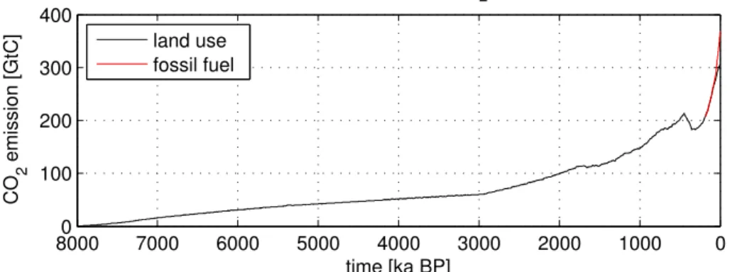
timing of their CO₂ emissions. After 1765 (or 185 a BP) we add historical emissions from fossil fuel use from the RCP database (Meinshausen et al., 2011). The adopted cumulative emissions are shown in Fig. 2. For simplicity CO₂, emissions from land use changes are added to the atmospheric CO₂, i.e., we do not change the land carbon stocks when emitting CO₂from land use changes. This simplification will lead to a slight

5

overestimate of the carbon uptake by vegetation through CO₂ fertilisation, though we judge its impact to be minor. Both land use and fossil fuel emissions are assumed to have a δ13CO₂of −25 ‰.

2.5 Ice core data

We compare the atmospheric CO₂ concentrations from our experiments to CO₂

con-10

centration reconstructions from ice cores. For the Holocene, we use the CO₂ recon-struction by Monnin et al. (2004), obtained by analysing ice cores from Dome Con-cordia (EDC) and Dronning Maud Land. From their reconstruction we use the CO₂ concentration from EDC and the corresponding one sigma error bars. For the most recent times, we extend their time series by using data from Law Dome published by

15

Etheridge et al. (1996), who provide CO₂concentration only. For δ13CO₂, we compare to the data obtained from EDC by Elsig et al. (2009), including their error estimate.

For the Eemian, we compare with data by Schneider et al. (2013) for both CO₂and

δ13 CO₂. This data was also obtained from EDC, and error estimates from sample replication are provided for most of the data points. For MIS 11, we use the data from

20

the EDC (Siegenthaler et al., 2005) and Vostok (Petit et al., 1999; Raynaud et al., 2005) ice cores on the EDC3 gas age time scale, as published by Lüthi et al. (2008). For this data no detailed error estimate is provided, though Petit et al. estimate an error range of ±2–3 ppmv.

(11)

CPD

Full Screen / Esc

Printer-friendly Version Interactive Discussion Discussion P a per | Discussion P a per | Discussion P a per | Discussion P a per | 2.6 Model experiments

We aim to initialise the model to conditions early in the interglacial but after the large transient changes associated with the deglaciation are over. For the Holocene this implies starting the model simulation at 8 ka BP, when most of the ice sheets have melted and the initial regrowth of vegetation is finished. For the Eemian we begin the

5

model experiment at 126 ka BP, after the large transient peak in CO₂has decayed, and for MIS 11 we start the model at 420 ka BP. From these starting points onward, we drive the model with orbital and other forcings as appropriate until the end of the experiment at 0 ka, 116, and 380 ka BP for the Holocene, the Eemian and MIS 11, respectively.

Since the carbon cycle cannot be regarded as being in equilibrium on multi-millennial

10

timescales, we initialized the model for our experiments with a similar procedure as in Kleinen et al. (2010). Firstly, the model was run with equilibrium conditions appropriate for the beginning of the respective interglacial, including constant CO₂ as diagnosed from ice cores for the time. Atmospheric δ13CO₂ was also initialized to the ice core value. In a second step, ocean alkalinity was increased to get a carbonate

sedimen-15

tation flux of 16 Tmol a−1 in the deep ocean and 2 Tmol a−1 on the shelves in order to simulate the maximum in CaCO₃preservation in the deep sea before the onset of the interglacial. The model was then run with prescribed CO₂ for 5000 years. This setup of initial conditions ensures that the ocean biogeochemistry is in equilibrium with the climate at the onset of the interglacial, while it is in transition from the glacial to

inter-20

glacial state thereafter. Initial times and CO₂concentrations are summarized in Table 1. After the climate model state for the beginning of the model experiment has been ob-tained, this climate state is used for a separate spin up of the LPJ DGVM to determine an appropriate vegetation distribution and land carbon storage for the beginning of the experiment. The length of this spin up is 2000 years.

25

Using these initial conditions, we perform experiments for the Holocene, the Eemian and MIS 11. For the Holocene, we perform four experiments to investigate the role of the various forcings in the interglacial carbon cycle: (1) a model experiment

(12)

contain-CPD

Full Screen / Esc

ing neither peat accumulation, nor CaCO₃ sedimentation, nor anthropogenic land use emissions. This experiment is purely driven by orbital forcing. We denote it HOL_ORB. (2) An experiment containing peat accumulation, but neither CaCO₃sedimentation nor anthropogenic land use emissions, denoted HOL_PEAT. (3) An experiment using all of the natural forcing mechanisms, i.e., peat accumulation and CaCO₃sedimentation,

5

denoted HOL_NAT. (4) The same setup as HOL_NAT, but also including anthropogenic carbon emissions, denoted HOL_ALL. Experiments for the Eemian and MIS11 follow the setup HOL_NAT with appropriate initial conditions, assuming that anthropogenic land use did not play a role then. In addition we performed an experiment for each interglacial, where we disabled the slow forcing factors as in set up HOL_ORB. The

10

characteristics of all experiments are summarised in Table 1.

All experiments are driven by orbital changes (Berger, 1978). The experiments that consider variable shallow-water CaCO₃accumulation rates (HOL_NAT, HOL_ALL, EEM_NAT, and MIS11_NAT) also require sea level changes, as described in Sect. 2.4, and in experiment HOL_ALL anthropogenic CO₂emissions from land use changes and

15

fossil fuel burning are provided as an additional forcing, as described in Sect. 2.4.

3 Results 3.1 Holocene

The model experiment HOL_ORB, without peat accumulation and CaCO₃ sedimen-tation in shallow waters, would correspond to the carbon cycle implemented in most

20

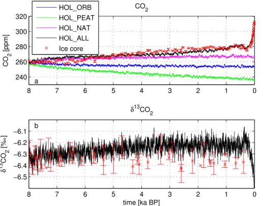
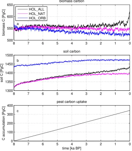
earth system models (ESM), i.e., a carbon cycle not taking into account slow pro-cesses of the C cycle. As shown in Fig. 3a, this model setup leads to a small decrease in CO₂ (∼ 5 ppm) over the first 2000 years, followed by constant CO₂ for the remain-der of the experiment. The modelled terrestrial biomass carbon decreases by about 30 Pg C during this time, as shown in Fig. 4a, while the soil carbon increases by a

sim-25

(13)

CPD

Full Screen / Esc

to minor changes in atmospheric CO₂, especially missing the increase in atmospheric CO₂by 20 ppm shown in the ice core record for 6 ka BP to 0 ka.

The results from model experiment HOL_PEAT, including carbon accumulation in boreal peatlands but excluding CaCO₃ accumulation in shallow waters, is shown in green in Fig. 3a. It exhibits an atmospheric CO₂ decrease by 25 ppm at 0 ka BP

rela-5

tive to 8 ka BP, which is explained by the uptake of 320 Pg C by peatland growth. Yu et al. (2010) estimate a total accumulation of 550 Pg C in northern peatlands from the LGM to the present, which indicates that the peat accumulation is reasonable in our model, considering the time frame of our experiment.

The results from our experiment HOL_NAT, including carbon storage in boreal

peat-10

lands and shallow water CaCO₃accumulation, are shown as a magenta line in Fig. 3a. Here, the trajectory of atmospheric CO₂ follows the ice core measurements rather closely until about 3 ka BP. Between 8 ka and 6 ka BP, the model overestimates CO₂by up to 5 ppm, while it underestimates atmospheric CO₂after 4 ka BP, with the discrep-ancy rising as the model gets closer to the present. Atmospheric CO₂stays constant

15

at 268 ppm after 4 ka BP in this experiment.

Finally, the results from HOL_ALL, i.e., a model setup similar to HOL_NAT but with anthropogenic emissions of CO₂ from land use changes and fossil fuel use consid-ered, are shown in black in Fig. 3a. Here the atmospheric CO₂is very similar to CO₂ in HOL_NAT until about 4 ka BP, after which HOL_ALL displays a continued increase

20

in CO₂, in line with ice core CO₂. The CO₂trajectory stays relatively close to the mea-surements over the entire time frame of the experiment, with a maximum deviation of about 8 ppm CO₂at 1.5 ka BP.

Biomass carbon, shown in Fig. 4a, stays nearly constant at 550 Pg C over the entire simulation period of experiment HOL_NAT, in contrast to the decrease observed for

25

HOL_ORB. For the first 5 ka, biomass carbon in HOL_ALL is very similar to HOL_NAT, but after 2.5 ka BP it increases driven by the increase in atmospheric CO₂, and reaches more than 600 Pg C at the end of the experiment. Soil carbon stocks, shown in Fig. 4b, initially are 110 Pg C lower in HOL_NAT and HOL_ALL than in HOL_ORB. This di

(14)

ffer-CPD

Full Screen / Esc

ence is due to the fact that some areas, especially in the high latitudes rich in soil C, are set aside as peatlands and therefore not available for mineral soil carbon storage. In experiment HOL_NAT the soil carbon stock increases from an initial 1325 to about 1400 Pg C at 0 ka. The evolution in HOL_ALL is very similar for the first 5 ka, but after 3 ka BP soil carbon increases more than in HOL_NAT due to higher CO₂, and reaches

5

a maximum of 1425 Pg C at the end of the experiment.

Figure 3b shows the carbon 13 isotope of CO₂, δ13CO₂from experiment HOL_ALL (black) in comparison to ice core measurements from EDC (Elsig et al., 2009) (red). Modelled δ13CO₂mostly stays within the range of the error bars before 4.5 ka BP, and only after 3 ka BP is the model δ13CO₂consistently above the range of the error bars.

10

Overall, the model setup HOL_ALL therefore captures changes in atmospheric CO₂ as measured from Antarctic ice cores reasonably well, though there is a divergence in

δ13CO₂after 3 ka BP.

Figure 4c shows the cumulative carbon uptake by peatlands in experiments HOL_NAT and HOL_ALL. Carbon storage in peatlands increases nearly linearly over

15

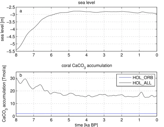
the entire time of the experiment (in fact, carbon uptake only saturates after several tens of ka), up to a total of 330 Pg C accumulated at the end of experiment HOL_ALL, while HOL_PEAT (not shown) accumulated 320 Pg C. The difference is due to the fertilisation effect of CO₂on photosynthesis. Sea level initially rises fast (see Fig. 5a), reaching sta-ble levels around 5 ka BP. The CaCO₃accumulation rate, shown in Fig. 5b, varies with

20

the rate of sea level change. The rate of sea level change is highest early during the Holocene, about 2 mm a−1, leading to a CaCO₃ sedimentation of about 27 Tmol a−1. Sea level stabilises later in the Holocene, leading to a CaCO₃ sedimentation of about 15 Tmol a−1.

3.2 Eemian

25

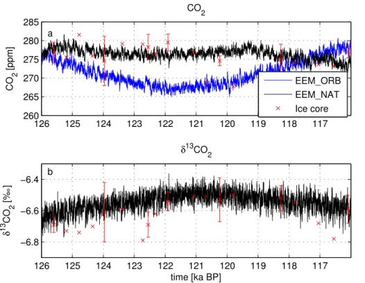
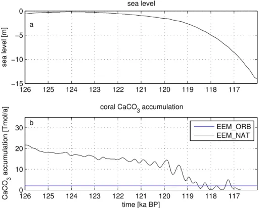
We consider the full natural setup of the model for the Eemian in experiment EEM_NAT, similar to experiment HOL_NAT. In Fig. 6 we show atmospheric CO₂ and δ13CO₂ as

(15)

CPD

Full Screen / Esc

simulated by the model in comparison to the ice core data from Schneider et al. (2013). Modelled atmospheric CO₂ is generally within the range spanned by the error bars of the measurements, with few exceptions. Similarly, modelled δ13CO₂is within the range of the error bars for most of the measurements.

In contrast, experiment EEM_ORB, shown as a blue line in Fig. 6a, is not able to

5

explain the CO₂ trajectory as reconstructed from the ice core. Here, CO₂ decreases from the initial value of 276 to about 267 ppm CO₂at 121 ka BP, after which it increases again to 278 ppm at 116 ka BP. While the discrepancy in CO₂ between experiment EEM_ORB and the ice core data is not excessive, the fit of experiment EEM_NAT to the data is substantially better. The slow natural processes we consider therefore seem

10

to be required to explain the evolution of CO₂during the Eemian.

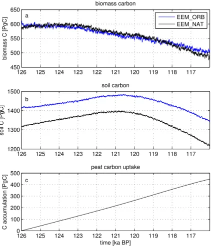
The terrestrial biomass (Fig. 7a) reaches a maximum of about 600 Pg C early in ex-periment EEM_NAT at 124 ka BP. It decreases thereafter and reaches a minimum value of ∼ 490 Pg C at the end of the experiment at 116 ka BP. Biomass carbon in experiment EEM_ORB follows a very similar trajectory. Soil carbon in EEM_NAT (Fig. 7b) increases

15

from an initial value of 1325 to about 1400 Pg C at 121 ka BP and decreases thereafter, reaching 1225 Pg C at 116 ka BP. The evolution in EEM_ORB is similar, though offset by about 90 Pg C, again due to the larger area available for mineral soil carbon when no peatlands are considered. The carbon storage in peatlands, shown in Fig. 7c for EEM_NAT, increases linearly during the Eemian as well, until about 440 Pg C are

ac-20

cumulated at the end of the experiment.

The sea level forcing, shown in Fig. 8a, is stable early during the experiment and decreases after 121 ka BP. Therefore shallow water CaCO₃ accumulation (Fig. 8b) is at ∼ 20 Tmol a−1 during the early Eemian, lower than during the early Holocene. It decreases to about zero at 119 ka and stays at this level thereafter.

(16)

CPD

Full Screen / Esc

Printer-friendly Version Interactive Discussion Discussion P a per | Discussion P a per | Discussion P a per | Discussion P a per | 3.3 MIS 11

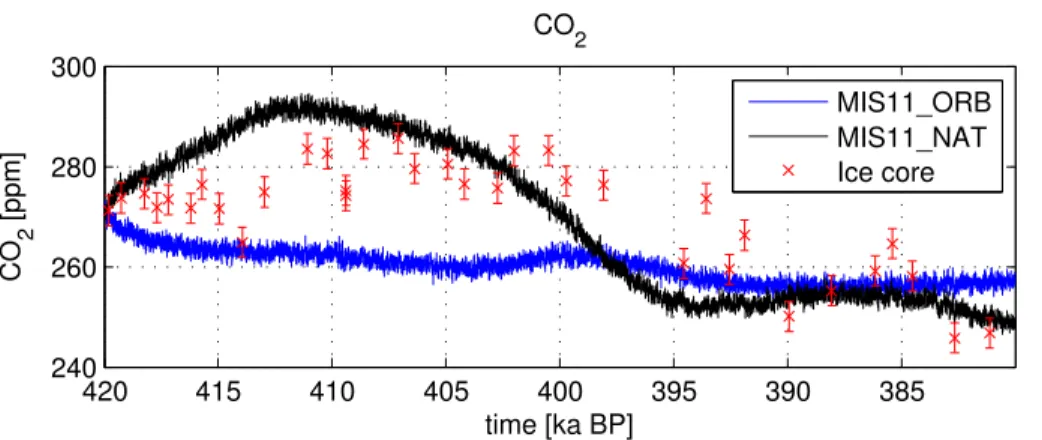
For MIS 11, the agreement between the modelled CO₂concentrations in MIS11_NAT and the ice core reconstruction is not as good as for the other two interglacials. As shown in Fig. 9 modelled CO₂in experiment MIS11_NAT increases initially from 271 to about 290 ppm at 412 ka BP. It declines thereafter to about 250 ppm CO₂at 395 ka BP,

5

after which CO₂ varies much less. Setup MIS11_ORB, on the other hand, shows a slowly decreasing trend in CO₂, from the initial 271 ppm CO₂ to slightly less than 260 ppm at 380 ka BP, with only little variation about this trend.

The initial increase in CO₂ is slower in the ice core data than in MIS11_NAT. CO₂ increases to about 285 ppm at 407 ka BP. Measured CO₂ decreases strongly after

10

398 ka BP, until 250 ppm CO₂ are reached at 390 ka BP. Therefore the model setup MIS11_NAT overestimates the initial increase in CO₂, and the peak in CO₂is reached about 5 ka earlier than in the ice core data. Similarly, the decrease after the peak in CO₂also occurs earlier in the model than in the ice core data. Nonetheless, the overall CO₂trajectory, with an initial increase in CO₂between 420 ka and 405 ka BP, followed

15

by a decrease by about 25–30 ppm and a stabilisation of CO₂ after 395 ka BP is cap-tured by MIS11_NAT, though the timing is not exactly the same as in the ice core data. MIS11_ORB, on the other hand, does not at all follow the ice core CO₂data.

The land carbon pools display substantially more variability in MIS11_NAT than in MIS11_ORB, shown in Fig. 10a and b. Biomass carbon (Fig. 10a) increases strongly

20

in MIS11_NAT, until a maximum value of about 630 Pg C is reached at 412 ka BP. Carbon storage decreases afterwards, until a minimum of 480 Pg C is reached at 395 ka BP, with only small changes afterwards. Similarly, soil carbon increases early in MIS11_NAT from an initial value of 1350 to about 1425 Pg C at 414 ka BP. It then stays constant until 403 ka BP, when it starts decreasing strongly. After 395 ka BP soil

25

carbon stays constant at 1345 Pg C. In contrast, the variations in biomass and soil carbon are much less pronounced in experiment MIS11_ORB. Biomass carbon in-creases from 540 to 560 Pg C early in MIS 11, then dein-creases again to 515 Pg C at

(17)

CPD

Full Screen / Esc

395 ka BP, and changes little afterwards. Soil carbon, on the other hand, varies be-tween 1490 and 1445 Pg C during the entire time frame of the experiment. Peat accu-mulation in MIS11_NAT (Fig. 10c) once again increases nearly linearly between 420 and 398 ka BP. After 398 ka BP the rate of increase decreases slightly due to the lower atmospheric CO₂concentration.

5

During the first 13 ka of MIS 11 sea level increases from −20 m to near zero (Fig. 11a). It starts decreasing again at 407 ka BP, but stabilises at −15 m after 395 ka BP. This sea level trajectory is reflected in the CaCO₃accumulation flux, shown in Fig. 11b: the initial fast rise in sea level leads to a accumulation rate of up to 29 Tmol a−1, which declines between 413 and 400 ka BP, when the accumulation rate is

10

zero due to the decrease in sea level. With the slowing rate of sea level decrease, sed-imentation increases again after 396 ka BP and reaches values of about 15 Tmol a−1 again at 390 ka BP.

4 Discussion

From our results for the Holocene carbon cycle, it becomes quite clear that all of the

15

forcings and processes considered taken together deliver the best match to the ice core CO₂data. The model setup HOL_ORB, i.e., a carbon cycle setup without anthro-pogenic CO₂ emissions or slow natural processes, leads to a more or less constant CO₂ trajectory, while the consideration of peat accumulation by itself in HOL_PEAT leads to a decrease in atmospheric carbon dioxide. The additional consideration of

20

CO₂ emissions from CaCO₃ shallow water sedimentation in HOL_NAT then leads to an increase in atmospheric CO₂, not just compensating the C uptake by peatlands, but also releasing additional CO₂to the atmosphere. From the difference between exper-iments HOL_NAT and HOL_ALL it becomes clear that anthropogenic CO₂ emissions from land use changes only make a significant difference to atmospheric CO₂ after

25

(18)

CPD

Full Screen / Esc

CO₂observed in ice cores between 8 and 4 ka BP. For the earlier Holocene CO₂ emis-sions from shallow water CaCO₃sedimentation are required instead.

While our CaCO₃accumulation model seems to capture the late Holocene sedimen-tation, with good agreement to Milliman (1993), the increase in accumulation rate due to the rate of sea level rise during the earlier Holocene is relatively uncertain. This is

5

due to uncertainties in the parameterisation, as well as uncertainties in the rate of sea level rise. While both are plausible, there is considerable uncertainty with respect to magnitude and timing of the CO₂emissions from CaCO₃formation. Previous assess-ments agree, though, that coral growth was stronger in the early Holocene (Ryan et al., 2001; Vecsei and Berger, 2004).

10

Finally, the modelled trajectory of δ13CO₂for the Holocene has relatively high values between 4 ka BP and the present, as shown in Fig. 4b. These values are outside the range of the error bars estimated by Elsig et al. (2009). This result can be explained in three different ways: (a) Elsig et al. might have underestimated the true uncertainty, (b) we may have underestimated the δ13CO₂ changes induced by the accumulation

15

of peat, and (c) we may require an unknown additional source of isotopically depleted carbon to explain the trajectory of δ13CO₂. This latter explanation has been favoured by proponents of large anthropogenic emissions from land-use changes, since CO₂ released from the biosphere would have such a depleted isotopic signature (Ruddi-man et al., 2011). At 307 Pg C cumulative emissions from land use changes, the

sce-20

nario adopted here already assumes larger fluxes than other recent estimates. Stocker et al. (2014), for example, estimate the cumulative emissions by 2004 at 243 Pg C. Besides, judging from Fig. 4b, the modelled atmospheric δ13CO₂ is higher than the measurements after about 4.5 ka BP, earlier than the bulk of the emissions in the sce-nario based on Kaplan et al. (2011). Emissions from anthropogenic land use changes

25

therefore do not appear to be a likely cause of the mismatch in δ13C, but we cannot rule out other isotopically depleted sources of C, such as methane emissions or the release of carbon from thawing permafrost soils. With regard to (b), we assume that the car-bon uptake by peat accumulation has a similar signature in δ13C as the growth of C3

(19)

CPD

Full Screen / Esc

grass. Since photosynthesis in mosses generally follows the C3 pathway, this assump-tion appears reasonable, and values for δ13C in mosses reported in the literature (e.g. Waite and Sack, 2011) are in a similar range as values for other C3 vegetation. With regard to (a), finally, there are no reasons to believe that measurement errors are un-derestimated by Elsig et al. (2009), forcing us to reject (a) as well. This leaves unknown

5

sources of isotopically depleted C as the most likely explanation for the discrepancy in

δ13C.

With regard to the evolution of atmospheric CO₂during the Eemian, the fit between ice core data and model results is clearly better for experiment EEM_NAT than for EEM_ORB. While the model produces an initial decrease followed by an increase for

10

EEM_ORB, EEM_NAT shows a near constant CO₂ concentration for the entire time we modelled, very close to the measurements by Schneider et al. (2013). Similarly, modelled δ13CO₂ is within the error bars of the ice core measurements most of the time. Here the largest uncertainty in our setup again stems from the sea level history, leading to uncertainty with respect to magnitude and timing of CO₂ emissions that

15

result from CaCO₃ sedimentation. In our setup, and with the sea level forcing data we use, the CO₂ emissions from CaCO₃ sedimentation counterbalance the decrease in CO₂shown in setup EEM_ORB for the early Eemian, while carbon uptake by peatlands compensates for the increase in CO₂modelled in EEM_ORB during the second half of the Eemian.

20

For MIS 11 our model experiment MIS11_NAT displays a similar evolution of atmo-spheric CO₂as the ice core data, with an initial increase, followed by a decrease during the middle of the interglacial until the CO₂concentration stabilises for the later part of the interglacial. This leads to a clearly better fit to the ice core measurements than setup MIS11_ORB, which shows a continuous slow decrease in CO₂. Nonetheless

25

there still are discrepancies in the timing and the magnitude of the changes in CO₂ be-tween model and ice core data. This discrepancy is most likely again due to uncertainty in the sea level history that we use to force the model. If the increase in sea level before

(20)

CPD

Full Screen / Esc

410 ka BP were slightly less pronounced and the decrease in sea level after 405 ka BP slightly delayed, our model results would fit the ice core data even better.

Carbon uptake by peatlands does not change substantially, neither during any of the interglacials, nor between interglacials. In all cases we obtain a more or less linear rise in peatland carbon storage.

5

Our study has several other limitations. We imposed anthropogenic emissions from land use changes as a simple flux to the atmosphere without changing the land car-bon stocks. This simplification modifies the uptake of carcar-bon by the biosphere and should already be contained in the Kaplan et al. (2011) CO₂emission estimate, but an inconsistency remains nonetheless. We also neglected the long-term memory of the

10

carbonate compensation response to the release of carbon from the deep ocean and the early interglacial carbon uptake by the terrestrial biosphere during deglaciation. While CLIMBER2-LPJ contains all relevant processes, we did not model this period transiently and therefore do not have the long-term memory signal in our results. Men-viel and Joos (2012) found that these memory effects could be of the order of few

15

ppm for the Holocene. Furthermore we assumed that the long-term carbon cycle was in equilibrium in the pre-industrial climate, but this assumption is a simplification as the balance among carbonate burial, weathering, and volcanic outgassing could be out of equilibrium for other climates. As follows from control simulations without forc-ings (not shown), these effects can be of the order of few ppm as well. Last but not

20

least, several other mechanisms that are currently under discussion such as changes in permafrost carbon pools (Schneider von Deimling et al., 2012) or methane hydrate storages (Archer et al., 2009) are not accounted for, as modelling of these processes is still in an early stage and because of the lack of reliable constraints on the amplitude of interglacial changes in these potentially large carbon pools.

(21)

CPD

Full Screen / Esc

Printer-friendly Version Interactive Discussion Discussion P a per | Discussion P a per | Discussion P a per | Discussion P a per | 5 Conclusions

We show – to our knowledge for the first time – how the trends in interglacial atmo-spheric CO₂, as reconstructed from ice cores, can be reproduced by a climate model with identical forcing parameterisation for three recent interglacials. For these trends in atmospheric CO₂ it is important to account not just for the marine and terrestrial

5

carbon cycle components, as implemented in most earth system models (Ciais et al., 2013). Instead, it is necessary to also consider the two slow processes of CO₂change currently neglected in the most comprehensive carbon cycle models, namely the car-bon accumulation in peatlands and the CO₂release from CaCO₃formation and burial in shallow waters. This latter process leads to an increase in atmospheric CO₂

dur-10

ing periods of constant or slowly rising sea level, while the former process leads to a decrease in atmospheric CO₂.

For the Holocene, we can explain the rise in atmospheric CO₂between 8 and 3 ka BP purely by natural forcings, while later in the Holocene, starting at about 3 ka BP, anthro-pogenic emissions from land use changes and fossil fuel use play an important role.

15

The increase in atmospheric CO₂ during the early Holocene therefore is the result of enhanced shallow water sedimentation of CaCO₃ due to rising sea level. For the Eemian, our carbon cycle model also leads to a satisfactory simulation of atmospheric CO₂, which is very close to the ice core data. Here the consideration of the slow carbon cycle processes also led to an improvement over the conventional model. For MIS 11,

20

finally, the conventional model setup does not simulate the changes in CO₂ observed throughout MIS 11, while the model with consideration of the slow forcings can explain the magnitude of changes in atmospheric CO₂, though the timing of changes is slightly different from the ice core data. This discrepancy is possibly due to the sea level forcing history that we use to drive the shallow water CaCO₃accumulation in our model, and

25

which remains uncertain.

Despite the uncertainties discussed above, we can draw some robust conclusions with regard to the timing of CO₂changes. Early during interglacials, when sea level still

(22)

CPD

Full Screen / Esc

rises, shallow water accumulation of CaCO₃and the related CO₂release is larger than in periods of stagnating or receding sea level. The carbon uptake by peatlands, on the other hand, is a more or less constant forcing factor. This uptake balances the CO₂ emission from CaCO₃ precipitation during periods of constant sea level. A rising sea level therefore leads to atmospheric CO₂increases, while a decline in sea level strongly

5

reduces shallow-water CaCO₃ sedimentation, leading to a reduction in atmospheric CO₂.

Acknowledgements. T. Kleinen acknowledges support through the DFG (Deutsche Forschungsgemeinschaft) priority research program INTERDYNAMIK. G. Munhoven is a Research Associate with the Belgian Fonds de la Recherche Scientifique – FNRS. We thank 10

Katharina Six for providing valuable comments on an earlier version of this manuscript. We also thank Dallas Murphy and Jochem Marotzke, as well as the participants of the scientific writing workshop at the MPI for Meteorology, whose comments on style led to substantial improvements of the present text.

15

The article processing charges for this open-access publication were covered by the Max Planck Society.

References

Archer, D.: A data-driven model of the global calcite lysocline, Global Biogeochem. Cy., 10, 511–526, 1996.

20

Berger, A.: Long-term variations of daily insolation and Quaternary climatic changes, J. Atmos. Sci., 35, 2362–2367, 1978.

Brovkin, V., Bendtsen, J., Claussen, M., Ganopolski, A., Kubatzki, C., Petoukhov, V., and An-dreev, A.: Carbon cycle, vegetation, and climate dynamics in the Holocene: experiments with the CLIMBER-2 model, Global Biogeochem. Cy., 16, 1139, doi:10.1029/2001GB001662, 25

2002.

Brovkin, V., Ganopolski, A., Archer, D., and Rahmstorf, S.: Lowering of glacial atmospheric CO₂ in response to changes in oceanic circulation and marine biogeochemistry, Paleoceanogra-phy, 22, PA4202, doi:10.1029/2006PA001380, 2007.

(23)

CPD

Full Screen / Esc

Brovkin, V., Ganopolski, A., Archer, D., and Munhoven, G.: Glacial CO₂cycle as a succession of key physical and biogeochemical processes, Clim. Past, 8, 251–264, doi:10.5194/cp-8-251-2012, 2012.

Buddemeier, R. W. and Smith, S. V.: Coral reef growth in an era of rapidly rising sea level: predictions and suggestions for long-term research, Coral Reefs, 7, 51–56, 1988.

5

Ciais, P., Sabine, C., Bala, G., Bopp, L., Brovkin, V., Canadell, J., Chhabra, A., DeFries, R., Gal-loway, J., Heimann, M., Jones, C., Le Quéré, C., Myneni, R. B., Piao, S., and Thornton, P.: Carbon and other biogeochemical cycles, in: Climate Change 2013: The Physical Science Basis. Contribution of Working Group I to the Fifth Assessment Report of the Intergovern-mental Panel on Climate Change, edited by: Stocker, T. F., Qin, D., Plattner, G.-K., Tignor, M., 10

Allen, S. K., Boschung, J., Nauels, A., Xia, Y., Bex, V., and Midgley, P. M., Cambridge Univer-sity Press, Cambridge, UK and New York, NY, USA, 465–570, 2013.

Elsig, J., Schmitt, J., Leuenberger, D., Schneider, R., Eyer, M., Leuenberger, M., Joos, F., Fis-cher, H., and Stocker, T. F.: Stable isotope constraints on Holocene carbon cycle changes from an Antarctic ice core, Nature, 461, 507–510, 2009.

15

Etheridge, D. M., Steele, L. P., Langenfelds, R. L., Francey, R. J., Barnola, J.-M., and Mor-gan, V. I.: Natural and anthropogenic changes in atmospheric CO2over the last 1000 years

from air in Antarctic ice and firn, J. Geophys. Res., 101, 4115–4128, 1996.

Frankignoulle, M., Canon, C., and Gattuso, J.-P.: Marine calcification as a source of carbon dioxide: positive feedback of increasing atmospheric CO₂, Limnol. Oceanogr., 39, 458–462, 20

1994.

Ganopolski, A. and Calov, R.: The role of orbital forcing, carbon dioxide and regolith in 100 kyr glacial cycles, Clim. Past, 7, 1415–1425, doi:10.5194/cp-7-1415-2011, 2011.

Ganopolski, A., Rahmstorf, S., Petoukhov, V., and Claussen, M.: Simulation of modern and glacial climates with a coupled global climate model, Nature, 391, 351–356, 1998.

25

Ganopolski, A., Petoukhov, V., Rahmstorf, S., Brovkin, V., Claussen, M., Eliseev, A., and Ku-batzki, C.: CLIMBER-2: a climate system model of intermediate complexity. Part II: Model sensitivity, Clim. Dynam., 17, 735–751, 2001.

Gerlach, T.: Volcanic versus anthropogenic carbon dioxide, EOS T. Am. Geophys. Un., 92, 201–202, 2011.

30

Gerten, D., Schaphoff, S., Haberlandt, U., Lucht, W., and Sitch, S.: Terrestrial vegetation and water balance – hydrological evaluation of a dynamic global vegetation model, J. Hydrol., 286, 249–270, 2004.

(24)

CPD

Full Screen / Esc

Indermühle, A., Stocker, T. F., Joos, F., Fischer, H., Smith, H. J., Wahlen, M., Deck, B., Mas-troianni, D., Tschumi, J., Blunier, T., Meyer, R., and Stauffer, B.: Holocene carbon-cycle dy-namics based on CO2 trapped in ice at Taylor Dome, Antarctica, Nature, 398, 121– 126,

doi:10.1038/18158, 1999.

Joos, F., Gerber, S., Prentice, I. C., Otto-Bliesner, B. L., and Valdes, P. J.: Transient simula-5

tions of Holocene atmospheric carbon dioxide and terrestrial carbon since the Last Glacial Maximum, Global Biogeochem. Cy., 18, GB2002, doi:10.1029/2003GB002156, 2004. Kaplan, J. O., Krumhardt, K. M., Ellis, E. C., Ruddiman, W. F., Lemmen, C., and Klein

Gold-ewijk, K.: Holocene carbon emissions as a result of anthropogenic land cover change, Holocene, 21, 775–791, doi:10.1177/0959683610386983, 2011.

10

Kleinen, T., Brovkin, V., von Bloh, W., Archer, D., and Munhoven, G.: Holocene carbon cycle dynamics, Geophys. Res. Lett., 37, L02705, doi:10.1029/2009GL041391, 2010.

Kleinen, T., Brovkin, V., and Schuldt, R. J.: A dynamic model of wetland extent and peat accu-mulation: results for the Holocene, Biogeosciences, 9, 235–248, doi:10.5194/bg-9-235-2012, 2012.

15

Kleypas, J. A.: Modeled estimates of global reef habitat and carbonate production since the Last Glacial Maximum, Paleoceanography, 12, 533–545, 1997.

Lüthi, D., Le Floch, M., Bereiter, B., Blunier, T., Barnola, J.-M., Siegenthaler, U., Raynaud, D., Jouzel, J., Fischer, H., Kawamura, K., and Stocker, T. F.: High-resolution carbon diox-ide concentration record 650,000–800,000 years before present, Nature, 453, 379–382, 20

doi:10.1038/nature06949, 2008.

Meinshausen, M., Smith, S. J., Calvin, K. V., Daniel, J. S., Kainuma, M. L. T., Lamarque, J.-F., Matsumoto, K., Montzka, S. A., Raper, S. C. B., Riahi, K., Thomson, A. M., Velders, G. J. M., and van Vuuren, D.: The RCP greenhouse gas concentrations and their extension from 1765 to 2300, Climatic Change, 109, 213–241, doi:10.1007/s10584-011-0156-z, 2011.

25

Menviel, L. and Joos, F.: Toward explaining the Holocene carbon dioxide and carbon isotope records: results from transient ocean carbon cycle-climate simulations, Paleoceanography, 27, PA1207, doi:10.1029/2011PA002224, 2012.

Milliman, J. D.: Production and accumulation of calcium carbonate in the ocean: budget of a nonsteady state, Global Biogeochem. Cy., 7, 927–957, 1993.

30

Monnin, E., Steig, E. J., Siegenthaler, U., Kawamura, K., Schwander, J., Stauffer, B., Stocker, T. F., Morse, D. L., Barnola, J.-M., Bellier, B., Raynaud, D., and Fischer, H.: Evi-dence for substantial accumulation rate variability in Antarctica during the Holocene, through

(25)

CPD

Full Screen / Esc

synchronization of CO₂ in the Taylor Dome, Dome C and DML ice cores, Earth Planet. Sc. Lett., 224, 45–54, doi:10.1016/j.epsl.2004.05.007, 2004.

Munhoven, G. and François, L. M.: Glacial–interglacial variability of atmospheric CO2 due to

changing continental silicate rock weathering: a model study, J. Geophys. Res., 101, 21423– 21437, doi:10.1029/96JD01842, 1996.

5

New, M., Hulme, M., and Jones, P.: Representing twentieth-century space–time climate variabil-ity. Part II: Development of 1901–96 monthly grids of terrestrial surface climate, J. Climate, 13, 2217–2238, 2000.

Petit, J. R., Jouzel, J., Raynaud, D., Barkov, N. I., Barnola, J.-M., Basile, I., Benders, M., Chappellaz, J., Davis, M., Delayque, G., Delmotte, M., Kotlyakov, V. M., Legrand, M., 10

Lipenkov, V. Y., Lorius, C., Pépin, L., Ritz, C., Saltzman, E., and Stievenard, M.: Climate and atmospheric history of the past 420 000 years from the Vostok ice core, Antarctica, Nature, 399, 429–436, 1999.

Petoukhov, V., Ganopolski, A., Brovkin, V., Claussen, M., Eliseev, A., Kubatzki, C., and Rahm-storf, S.: CLIMBER-2: a climate system model of intermediate complexity. Part I: Model de-15

scription and performance for present climate, Clim. Dynam., 16, 1–17, 2000.

Raynaud, D., Barnola, J.-M., Souchez, R., Lorrain, R., Petit, J.-R., Duval, P., and Lipenkov, V. Y.: The record for marine isotopic stage 11, Nature 436, 39–40, doi:10.1038/43639b, 2005. Ridgwell, A. J., Watson, A. J., Maslin, M. A., and Kaplan, J. O.: Implications of coral reef buildup

for the controls on atmospheric CO₂since the Last Glacial Maximum, Paleoceanography, 18, 20

1083, doi:10.1029/2003PA000893, 2003.

Ruddiman, W. F.: The anthropogenic greenhouse era began thousands of years ago, Climatic Change, 61, 261–293, doi:10.1023/B:CLIM.0000004577.17928.fa, 2003.

Ruddiman, W. F., Kutzbach, J. E., and Vavrus, S. J.: Can natural or anthropogenic expla-nations of late-Holocene CO₂ and CH₄ increases be falsified? Holocene, 21, 865–8879, 25

doi:10.1177/0959683610387172, 2011.

Ryan, D. A., Opdyke, B. N., and Jell, J. S.: Holocene sediments of Wistari Reef: towards a global quantification of coral reef related neritic sedimentation in the Holocene, Palaeo-geogr. Palaeocl., 175, 173–184, 2001.

Schneider, R., Schmitt, J., Köhler, P., Joos, F., and Fischer, H.: A reconstruction of atmospheric 30

carbon dioxide and its stable carbon isotopic composition from the penultimate glacial max-imum to the last glacial inception, Clim. Past, 9, 2507–2523, doi:10.5194/cp-9-2507-2013, 2013.

(26)

CPD

Full Screen / Esc

Schneider von Deimling, T., Meinshausen, M., Levermann, A., Huber, V., Frieler, K., Lawrence, D. M., and Brovkin, V.: Estimating the near-surface permafrost-carbon feedback on global warming, Biogeosciences, 9, 649–665, doi:10.5194/bg-9-649-2012, 2012.

Scholze, M., Kaplan, J. O., Knorr, W., and Heimann, M.: Climate and interannual variability of the atmosphere–biosphere 13CO₂ flux, Geophys. Res. Lett., 30, 1097, 5

doi:10.1029/2002GL015631, 2003.

Schurgers, G., Mikolajewicz, U., Gröger, M., Maier-Reimer, E., Vizcaíno, M., and Winguth, A.: Dynamics of the terrestrial biosphere, climate and atmospheric CO₂ concentration dur-ing interglacials: a comparison between Eemian and Holocene, Clim. Past, 2, 205–220, doi:10.5194/cp-2-205-2006, 2006.

10

Siegenthaler, U., Stocker, T. F., Monnin, E., Lüthi, D., Schwander, J., Stauffer, B., Raynaud, D., Barnola, J.-M., Fischer, H., Masson-Delmotte, V., and Jouzel, J.: Stable carbon cycle-climate relationship during the late pleistocene, Science, 310, 1313–1317, 2005.

Sitch, S., Smith, B., Prentice, I. C., Arneth, A., Bondeau, A., and Cramer, W., Cramer, W., Kaplan, J. O., Levis, S., Lucht, W., Sykes, M., Thonicke, K., and Venevsky, S.: Evaluation 15

of ecosystem dynamics, plant geography and terrestrial carbon cycling in the LPJ dynamic global vegetation model, Glob. Change Biol., 9, 161–185, 2003.

Stocker, B. D., Feissli, F., Strassmann, K. M., Spahni, R., and Joos, F.: Past and future carbon fluxes from land use change, shifting cultivation and wood harvest, Tellus B, 66, 23188, doi:10.3402/tellusb.v66.23188, 2014.

20

US Department of Commerce, National Oceanic and Atmospheric Administration, National Geophysical Data Center: 2-minute Gridded Global Relief Data (ETOPO2v2), 2006.

Vecsei, A. and Berger, W. H.: Increase of atmospheric CO₂during deglaciation: constraints on the coral reef hypothesis from patterns of deposition, Global Biogeochem. Cy., 18, GB1035, doi:10.1029/2003GB002147, 2004.

25

Waelbroeck, C., Labeyrie, L., Michel, E., Duplessy, J. C., Mc-Manus, J. F., Lambeck, K., Bal-bon, E., and Labracherie, M.: Sea-level and deep water temperature changes derived from benthonic foraminifera isotopic records, Quaternary Sci. Rev., 21, 295–305, 2002.

Waite, M. and Sack, L.: Shifts in bryophyte carbon isotope ratio across an elevation x soil age matrix on Mauna Loa, Hawaii: do bryophytes behave like vascular plants?, Oecologia, 166, 30

(27)

CPD

Full Screen / Esc

Yu, Z., Loisel, J., Brosseau, D. P., Beilman, D. W., and Hunt, S. J.: Global peat-land dynamics since the Last Glacial Maximum, Geophys. Res. Lett., 37, L13402, doi:10.1029/2010GL043584, 2010.

(28)

CPD

Full Screen / Esc

Table 1. Setup of experiments performed for the Interglacials, including the forcing factors

var-ied.

Name Interglacial Initial CO2 Initial δ 13

CO2 Initial time Peat accumu- Coral CaCO3 Anthropogenic land

[ppm] [‰] [ka BP] lation sedimentation use emissions

HOL_ORB Holocene 260 −6.4 8 No No No

HOL_PEAT Holocene 260 −6.4 8 Yes No No

HOL_NAT Holocene 260 −6.4 8 Yes Yes No

HOL_ALL Holocene 260 −6.4 8 Yes Yes Yes

EEM_ORB Eemian 276 −6.7 126 No No No

EEM_NAT Eemian 276 −6.7 126 Yes Yes No

MIS11_ORB MIS11 271 – 420 No No No

(29)

CPD

Full Screen / Esc

−10

0

10

20

0.2

0.4

0.6

0.8

1 Rate of sea level rise [mm/a]

Coral

growth

mod

ifier

SLR dependent coral growth

Figure 1. Coral growth modification function. CaCO₃sedimentation is limited in cases of neg-ative and very fast sea level rise.

(30)

CPD

Full Screen / Esc

Printer-friendly Version Interactive Discussion Discussion P a per | Discussion P a per | Discussion P a per | Discussion P a per | 0 1000 2000 3000 4000 5000 6000 7000 80000 100 200 300 400

cumulative anthropogenic CO₂emissions

CO 2 emission [GtC] time [ka BP] land use fossil fuel

Figure 2. Cumulative anthropogenic carbon emissions from land use (black) and land use and

(31)

CPD

Full Screen / Esc

Printer-friendly Version Interactive Discussion Discussion P a per | Discussion P a per | Discussion P a per | Discussion P a per | 0 1 2 3 4 5 6 7 8 240 260 280 300 320 a CO₂ CO 2 [ppm] HOL_ORB HOL_PEAT HOL_NAT HOL_ALL Ice core 0 1 2 3 4 5 6 7 8 −6.5 −6.4 −6.3 −6.2 −6.1 b δ13CO₂ time [ka BP] δ 13 CO 2 [%°]

Figure 3. Holocene CO₂concentration(a) and δ13of CO₂(b) from EPICA Dome C (red) and

Siple Dome, model with all forcings HOL_ALL (black), model without anthropogenic forcing HOL_NAT (magenta), model without anthropogenic, peat and coral forcing HOL_ORB (blue), model without coral and anthropogenic forcing HOL_PEAT (green).

(32)

CPD

Full Screen / Esc

Printer-friendly Version Interactive Discussion Discussion P a per | Discussion P a per | Discussion P a per | Discussion P a per | 0 1 2 3 4 5 6 7 8 500 550 600 650 a biomass C [PgC] biomass carbon HOL_ALL HOL_NAT HOL_ORB 0 1 2 3 4 5 6 7 8 1300 1350 1400 1450 1500 b soil C [PgC] soil carbon 0 1 2 3 4 5 6 7 8 0 100 200 300 400 c time [ka BP] C accumulation [P gC]

peat carbon uptake

Figure 4. Land carbon pools in Holocene experiments HOL_ALL, HOL_NAT and HOL_ORB:

total biomass carbon(a), total non-peat soil carbon (b), and cumulative C uptake by peatlands (c).