A bi-value coding parameterization scheme for the discrete optimal
orientation design of the composite laminate
GAO Tong
1, 2, ZHANG Weihong
1,*, DUYSINX Pierre
21 Northwestern Polytechnical University, Xi’an, China
2 LTAS - Ingénierie des Véhicules Terrestres, Université de Liège, 4000 Liège, Belgium
* Corresponding author
Abstract
The discrete optimal orientation design of the composite laminate can be treated as a material selection problem dealt with by continuous topology optimization method. In this work, a new bi-value coding parameterization (BCP) scheme is proposed to this aim. The idea of the BCP scheme is to “code” each material phase using integer values of +1 and -1. Each available material phase has one unique “code” consisting of +1 and/or -1 assigned to design variables. Theoretical and numerical comparisons between the proposed BCP scheme and existing schemes show that the BCP has the advantage of an evident reduction of the number of design variables in logarithmic form. This is very beneficial when the number of candidate materials becomes important. Numerical tests with up to 36 candidate material orientations are illustrated for the first time to indicate the reliability and efficiency of the proposed scheme in solving this kind of problem. It proves that the BCP is an interesting and potential scheme to achieve the optimal orientations for large-scale design problems.
Key words
composite laminate, topology optimization, material selection, optimal orientation design, bi-value coding parameterization1. Introduction
In aerospace industry, composite materials are increasingly applied in the design of advanced aircraft and spacecraft because of their excellent properties and structural performances for the expected lighter and stiffer structures. Among others, laminate design is becoming a challenging research topic owing to its important role and the avoidance of local optimum solutions for the fiber orientation angles is a common problem. The advanced design approach resorts to the discrete orientation optimization that transforms the continuous orientation angle design as an optimal selection among a set of fiber angle values discretized a priori. The problem may refer to the optimal selection of fiber angles over a single laminate layer or the optimal stacking sequence of a multi-layer laminate. Generally speaking, following design methods are available to solve the discrete orientation problem.
The evolutionary techniques, such as the genetic algorithms (GAs, [1-3]), are popularly used, especially in stacking sequence optimization. The main advantages of the evolutionary techniques are twofold. Firstly, these methods are intuitively global optimization methods. Secondly, applications can be made for complicated structural responses and design constraints whose sensitivities are extremely difficult to calculate or even impossible. However, the evolutionary techniques are limited for small-scale problems due to the exhaustive computing time although the global optimum is sought for theoretically. Additionally, when the stacking sequence and orientation distribution are optimized simultaneously, the computing time will become prohibitive. Actually, if each orientation is treated as one material phase, the discrete optimal orientation design can be handled as a structural optimization problem with multiple materials. Within this framework, a suitable design method is to adopt interpolation models. The study of multiphase materials was firstly addressed by Thomsen [4]. And then Sigmund and co-workers ([5-7]) expanded the popular SIMP (Solid Isotropic Material with Penalization) to interpolate material properties of two solid material phases and void. A so-called peak function was presented by Yin and Ananthasuresh [8] to interpolate the properties of multiphase isotropic materials. Jung and Gea [9] constructed a variable-inseparable multiple material model for the design of
energy-absorbing structures. Mei and Wang [10] utilized the vector level set to implicitly describe the interfaces between two distinct material phases in structural topology optimization. These researches are basically oriented to solve topology optimization problem with multiple isotropic materials, they might be introduced into the design of discrete optimal orientation problem.
It is necessary to mention the work of Lund and co-workers [11-13] who proposed s series of parameterization schemes to treat the laminate design of composite materials as a discrete material optimization (DMO) problem. Recently, Bruyneel [14] introduced an interesting alternative parameterization scheme named shape function parameterization (SFP) for the design problem of four candidate orientations (0°, 90° and ±45°). Compared with the DMO scheme, the size of the optimization problem is halved by the SFP model. Usually, all these methods cannot guarantee the global optimum theoretically and the results depend on the chosen material interpolation strategy. Besides, the structural responses and design constraints involved until now are still limited by these methods.
In the earlier days, the so-called strain-based [15-17] and stress-based [17-19] methods were also developed to solve the optimal orientation problems. Because the strain field is more sensitive to the orientation variable than the stress field, the stress-based method can provide better results. However, when the concept of patches consisting of a set of finite elements is concerned for the design of fiber orientation angles, the stress-based method associated to the principal stress and strain of each finite element is no longer applicable.
In this paper, a new BCP scheme is proposed to interpolate the properties of multiple materials for the discrete optimal orientation design. The basic idea of this parameterization scheme is to define each material phase with a unique “code” consisting of all design variables. Numerical examples with up to 36 candidate orientations are tested to find the optimal orientations in a planar laminate layer. It is illustrated that the BCP scheme could largely reduce the size of the optimization problem containing a large number of discrete candidate orientations.
2. Discrete material parameterization model
2.1 DMO and SFP schemes
The discrete optimal orientation design of the laminate can be treated as an optimization problem with multiple materials or a problem of optimal material selection. Among others, the so-called DMO developed by Stegmann and Lund [20] is a typical scheme. As the weighting function in this method is uniform for each candidate material phase, the interpolation scheme is here referred to as uniform multiphase materials interpolation (UMMI).
For an optimal design problem with m available candidate orientations at each designable element or region, the UMMI is expressed as the weighted sum of all candidate material phases at element i. ( ) 1 m j i ij i j
c
w c
==
∑
(1) where the weighting function wij associated with the jth material phase should satisfy0
≤
w
ij≤
1
(2) and 11
m ij jw
=≤
∑
(3) Besides, if the following condition holds automatically(
)
0
i
w
ξ=
ξ
≠
j
whenw
ij=
1
(4) additional constraints are not needed in the optimization process to ensure the unique presence of a single material phase at each designable element. This is because other material phases will automatically become inactive.Stegmann and Lund [12] presented several DMO interpolation models, among which the typical one is
(
)
v 11
0
1
m p p ij ij i j ijw
x
x
x
ξ ξ ξ=≠=
−
≤
≤
∏
(5)In this scheme, the number of design variables attached to each designable element or region just equals the number of candidate material phase, i.e., mv=m.
Recently, Bruyneel [14] presented an alternative parameterization model named SFP based on the shape functions of finite element. For a design problem with 0°, 90° and ±45° plies, the shape functions of four-node element were introduced as,
(
)(
)
(
)(
)
(
)(
)
(
)(
)
1 1 2 2 1 2 3 1 2 4 1 21
1
1
1
1
1
4
4
1
1
1
1
1
1
4
4
1
1,
1, 2,3, 4
p p i i i i i i p p i i i i i i ijw
x
x
w
x
x
w
x
x
w
x
x
x
j
⎡
⎤
⎡
⎤
=
⎢
−
−
⎥
=
⎢
+
−
⎥
⎣
⎦
⎣
⎦
⎡
⎤
⎡
⎤
=
⎢
+
+
⎥
=
⎢
−
+
⎥
⎣
⎦
⎣
⎦
− ≤
≤
=
(6)Obviously, the conditions related to eqs. (2), (3) and (4) are satisfied by the above shape functions. Distinctly, only two variables are involved for four fiber orientations. This is the advantage over the DMO schemes in the size reduction of the optimization problem. As indicated in [14], the SFP could certainly be extended to more than four materials based on the existing finite element shape functions with two, three and eight nodes (bar, triangle membrane, and hexagonal volume element, respectively). The disadvantage is also obvious. Specific shape functions related to more complicated finite elements have to be sought out and constructed depending upon the number of material orientations involved in the design problem. Besides, to satisfy the conditions of eq.(2), (3) and (4), not all finite elements can be accepted for the SFP model and the shape functions must be chosen carefully.
2.2 Bi-value coding parameterization (BCP) scheme
The essential difference can be noticed below. In DMO scheme, the presence of one material phase is characterized by a specific design variable with unity value and other variables with zero value. Comparatively, in SFP scheme, the presence of one material phase is characterized by a specific combination of design variables taking bi-values of +1 and/or -1. Therefore, only two variables are needed for four materials.
To overcome the shortcoming of SFP scheme, one can sweep away the idea of shape functions resulting from the concept of a physical finite element from our mind and keep in mind only the idea of defining the shape function using bi-value of +1 and -1. Thus, a new BCP scheme is proposed here as the material parameterization model for m material phases,
(
)
v 1 v1
1
2
1
1
1, ,
v p m i j m jk ik k ikw
s x
x
k
m
=⎡
⎤
=
⎢
⋅
+
⎥
⎣
⎦
− ≤
≤
=
∏
"
(7)where mv, the number of design variables for designable element or area i, is an integer defined by
the ceiling function of lg2m
v
lg
2m
= ⎡
⎢
m
⎤
⎥
(8) In other words, the BCP scheme makes it possible to interpolatem
=
⎡
2
(mv−1)+
1, 2
mv⎤
⎣
⎦
materialphases with mv design variables.
The sjk values can be calculated in the following manner
2 1 1 log
1
1, 2
1
2 , 2
2
1, 2
vwhere
2
1
k k k jk j m k kj
s
j
s
ξj
ξ
j
− − ⎡ ⎤ ⎢ ⎥⎧
∈ ⎣
⎡
⎤
⎦
⎪⎪
⎡
⎤
= −
⎨
∈
⎣
⎦
⎪
⎡
⎤
∈
+
=
+ −
⎪
⎣
⎦
⎩
(9)For example, we have mv=4 for 9≤m≤16. The value of
s
jkis equal to 1 or -1. Herein, the penalization factor p is applied to push the design variables to their extreme values. Actually, the idea of this scheme is to “code” each material phase using the design variables. Here, one material phase is not able to be indicated any more by a single variable. Each available material phase has one unique “code” consisting of all variables with a combined value of -1/1.In BCP scheme, we have 0≤1+sjkxik≤2 due to the values of sjk and xik. Thus, the conditions related to eq.(2) and eq.(3) are obviously satisfied. Besides, because each material has a unique code, it can be mathematically derived that wiξ=0 (ξ≠j) if and only if wij=1. This means that when element i consists of material phase j, other material phases will automatically become inactive. The details of the “coding” scheme are discussed and illustrated below.
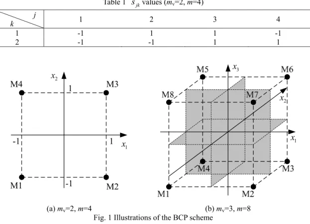
In the case of mv=2, the max number of candidate materials is m=4 and all corresponding values of
s
jk are listed in Table 1. Obviously, this material parameterization model is exactly the same as the SFP scheme presented in eq.(6) by Bruyneel [14]. To illustrate the “coding” clearly, a sketch is shown in Fig. 1(a). Each candidate material phase locates at the vertex of the square in the 2D coordinate system.Table 1
s
jkvalues (mv=2, m=4) j k 1 2 3 4 1 -1 1 1 -1 2 -1 -1 1 1M1
M2
M3
M4
1x
2x
-1
-1
1
1
1x
2x
3x
(a) mv=2, m=4 (b) mv=3, m=8Fig. 1 Illustrations of the BCP scheme
In the case of mv=3, m=8 for the max number of candidate materials and the corresponding
values of
s
jkare listed in Table 2. It is just like 3 coordinates planes dividing the 3D space into 8 quadrants. As shown in Fig. 1 (b), each of the 8 candidate material phase is just assigned to the vertex of a hexahedron in the 3D space consisting of three design variables.Table 2
s
jkvalues (mv=3, m=8) j k 1 2 3 4 5 6 7 8 1 -1 1 1 -1 -1 1 1 -1 2 -1 -1 1 1 1 1 -1 -1 3 -1 -1 -1 -1 1 1 1 1Similarly, for the max number of candidate materials m=16, we have mv=4 and
s
jkvalues are listed in Table 3. The same deduction can be made for more candidate material phases. Itshould be indicated that only terms
s
jk(j≤m) are used if2
(mv−1)+ ≤ <
1
m
2
mv. Table 3s
jkvalues (mv=4, m=16) j k 1 2 3 4 5 6 7 8 9 10 11 12 13 14 15 16 1 -1 1 1 -1 -1 1 1 -1 -1 1 1 -1 -1 1 1 -1 2 -1 -1 1 1 1 1 -1 -1 -1 -1 1 1 1 1 -1 -1 3 -1 -1 -1 -1 1 1 1 1 -1 -1 -1 -1 1 1 1 1 4 -1 -1 -1 -1 -1 -1 -1 -1 1 1 1 1 1 1 1 1 To have a clear idea, the number of design variables needed for DMO and BCP schemes is shown in Fig. 2. In the case of one or two available materials, the number of variables is the same for both schemes. However, the BCP scheme needs much less variables than DMO scheme in the case of m>2. Especially, the advantage of BCP scheme is greatly attractive if a great number of material phases is available. For example, for m=1000, we have only the number of design variables mv=10 for each designable element with BCP but mv=1000 with DMO.Fig. 2 Comparison of the number of design variables
3. Optimization design problem
Here, the minimum compliance design of laminated composite is considered with fiber angles to be optimized. Based on the above presentation, the optimization problem can be expressed as
{ } (
v)
T find: 1, , ; 1, , minimize: subject to: 1 1 ik ik x i n k m C x = = = = − ≤ ≤ F u F Ku " " (10)The sensitivity of the mean compliance can be generally expressed as
T T
2
ik ik ikC
x
x
x
∂
∂
∂
=
−
∂
∂
∂
F
K
u
u
u
(11) For fixed loads, then we have0
ik
x
∂
≡
∂
F
. Thus, the sensitivity can be simplified as
T T i i i ik ik ik
C
x
x
x
∂
∂
∂
= −
= −
∂
∂
∂
K
K
u
u
u
u
(12) For each finite element, the element stiffness matrix is interpolated using eq.Erreur ! Source du renvoi introuvable. so that the partial derivative can be calculated with( ) 1 m ij j i i j ik ik
w
x
=x
∂
∂
=
∂
∑
∂
K
K
(13) Using the proposed BCP scheme in eq.(7), we have(
)
1(
)
1 11
1
1
1
2
2
v v v v p m m ij j i jk j i m m ik kw
p
s x
s
s x
x
ξ ξ ξ ξ ξ ξ ξ − = = ≠∂
⎡
⎤
= ⋅
⎢
⋅
+
⎥
⋅
⋅
+
∂
⎣
∏
⎦
∏
(14)Obviously, p and (1+s xjξ iξ) in this expression are both positive, and then the sign of the partial
derivative ∂wij/∂xik depends on sjk. Anyway, wij is a monotonous function. However, the sensitivity ∂C/∂xik might be positive or negative due to the summation expression of the element stiffness matrix interpolation, which means the objective function might be non-monotonous and the local solutions might exist.
4. Numerical Examples
In this section, three numerical examples are tested to illustrate BCP scheme. Comparisons are also made to show its advantage. By applying the well-known concept of sequential convex programming (SCP), problem related to eq.(10) is dealt with by solving a sequence of convex subproblems involving only side constraints to design variables. In this paper, the structural analysis is carried out using SAMCEF finite element software and the GCMMA optimizer [23] is adopted to seek the optimal solution for each subproblem.
By virtue of eq.(10), the in-plane stiffness of the panel is maximized. Four cases of the candidate orientations listed in Table 4 are investigated to examine the capability of BCP scheme. The largest orientation number is up to 36. Herein, an orthotropic material is considered and its properties are listed in Table 5.
Table 4 Orientations Number of material phases (m) Number of design variables for each region (mv)
Discrete orientation angle (°)
4 2 90/45/0/-45
9 4 80/60/40/20/0/-20/-40/-60/-80
12 4 90/75/60/45/30/15/0/-15/-30/-45/-60/-75
18 5 90/80/70/60/50/40/30/20/10/0/-10/-20/-30/-40/-50/-60/-70/-80 36 6 -5/-10/-15/-20/-25/-30/-35/-40/-45/-50/-55/-60/-65/-70/-75/-80/-85 90/85/80/75/70/65/60/55/50/45/40/35/30/25/20/15/10/5/0/
Table 5 Material properties
Ex Ey Gxy vxy
146.86GPa 10.62GPa 5.45GPa 0.33
4.1 Square plate under horizontal traction
A square composite consisting of one ply is investigated. As shown in Fig. 3, the model is meshed with 16×16 quadrangular finite elements. The structure is clamped along the left edge and a uniform traction load is applied on the right edge. Besides, 16 separate designable patches are considered. It means the orientations in all elements of each patch are the same, while the orientations might be different between patches. The BCP scheme is adopted to parameterize the material properties.
1
2
3
4
5
6
7
8
9
10
11
12
13
14
15
16
Design model with 4×4 patches Loads and boundary conditions Fig. 3 Model of the square plate under horizontal traction
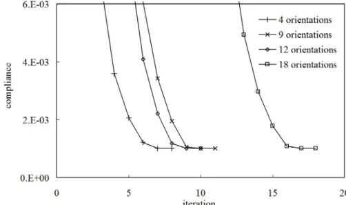
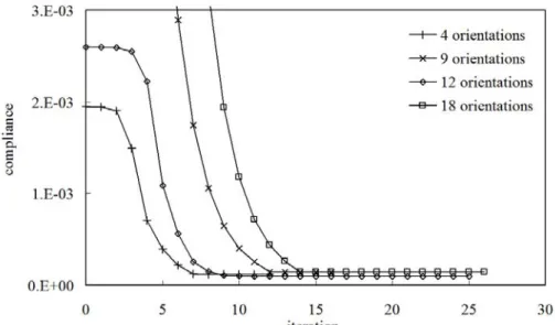
Four orientation cases listed in Table 4 are tested for m=4, 9, 12, 18. The iteration histories are plotted in Fig. 4. Although the orientations of each patch can be different and different orientation numbers are adopted at the beginning, the same optimal design only consisting of the material with an orientation of 0° is obtained over the whole structure. This design is obviously the expected optimum. It is found that the convergence rate depends on the number of design variables. A large value of mv means more iterations, while the influence of the number of candidate orientations, i.e., m upon the convergence rate is minor. For example, at m=9 and m=12, the optimization process converges after 11 and 10 iterations, respectively. The reason might be due to the same number of design variables (mv=4) in both cases.
Fig. 4 Iteration histories of the square plate under horizontal traction load (BCP)
4.2
Square plate under vertical forceFig. 5 Model of the square plate under vertical force
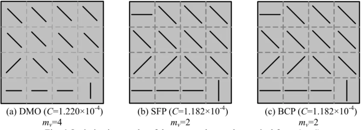
Here, the same structure is studied under a vertical force applied at the right-bottom point. The case of 4 orientations (m=4) is considered. The optimization results by DMO, SFP and BCP schemes are illustrated in Fig. 6. For this problem, 4 design variables are needed using DMO
scheme; while only 2 variables are needed for SFP and BCP schemes. It can be found that all solutions are nearly the same although small differences exist. Actually, BCP and SFP schemes result in exactly the same solution because both schemes are identical in this case. The result using SFP/BCP scheme is a little better according to the value of structural compliance. However, as the optimization algorithms the mostly used for structural design such as ConLin, MMA, GCMMA, MDQA are all based on the convex approximation and separable variables, no scheme can guarantee the global optimum theoretically.
(a) DMO (C=1.220×10⁻⁴) mv=4 (b) SFP (C=1.182×10⁻⁴) mv=2 (c) BCP (C=1.182×10⁻⁴) mv=2 Fig. 6 Optimization results of the square plate under vertical force (m=4)
Using the BCP scheme, the iteration histories of the weights for patch 16 are plotted in Fig. 7. At the starting point, all weights are exactly the same. Finally, orientation -45° is the optimum choice for this patch with the unit weight, while other weights gradually diminish to zero for the elimination of their effect. In fact, as the orientation 45° is the worst candidate compared to the orientation of -45°, the related weight evolves towards zero more quickly than other weights related to orientations of 0° and 90°.
Fig. 7 Iteration histories of the weight for patch 16 (BCP m=4)
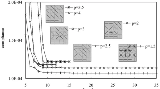
The influence of the penalization factor p on the optimization results is presented in Fig. 8. For different values of p, the optimization iterations are quite stable, while the compliances and orientation layouts are different in the optimization results. Generally, smaller penalization factor leads to stiffer design result. However, too small penalization factor makes the optimization iteration converge quite slowly. In the cases of p=2 and p=1.5, the optimization processes have not converged after 30 iterations, while the other tests need about 10 to 15 iterations. Besides, there are still some patches consisting of “mixed” material for these two tests after even 50 iterations, as shown in Fig. 8. In summary, the suggested value for the penalization factor is
p
∈
[
2.5, 4
]
.Fig. 8 Influence of the penalization factor p of the BCP scheme upon the optimization results In Fig. 9, several additional test results are shown with more orientations. The layout of the orientations in all optimization results is reasonable. The optimal layout with m=12 is stiffer than that with m=4 because more material orientations are available for the selection. In other words, the design space S(4) (m=4) is a sub-space of S(12) (m=12) with
S
( )4⊂
S
( )12 . For the resultcomparison with m=9 and m=18 candidate orientations, the optimal result related to m=18 is however worse than that of m=12 although the former has more available orientations than the latter. This is because both sets of material orientations have their specific orientations and are incomparable.
(a) m=9 (C=1.453×10⁻⁴) (b) m=12 (C=0. 954×10-4) (c) m=18 (C=1.424×10⁻⁴) Fig. 9 Optimization results of the square plate under vertical force using BCP)
Finally, the iteration histories for all orientation cases using BCP scheme are plotted in Fig. 10. Obviously, each optimization process converges in a stable and monotonous way.
Fig. 10 Iteration histories of the square plate under vertical force with BCP
4.3 Simply-supported beam
A simple-supported beam meshed with 240×40 quadrangular finite elements is shown in Fig. 11. Considering the symmetry, only a half of the whole structure is considered in the finite element analysis and optimization. Three patch partition cases and two candidate material orientation cases are investigated.
Fig. 11 Model of simply-supported beam
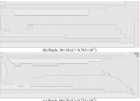
Firstly, optimization results using BCP scheme with m=4 candidate orientations are shown in Fig. 12. A reasonable layout of the orientations is achieved. With the increase of the designable patches, the design space of the optimization problem is enlarged. As a result, the global structural compliance decreases.
(b) Patch: 30×10 (C= 0.763×10⁻³)
(c) Patch: 60×20 (C= 0.731×10⁻³)
Fig. 12 Optimization results using BCP scheme (m=4)
Optimization results using BCP scheme with m=9 candidate orientations are shown in Fig. 13. What should be noticed is the gray area in Fig. 13(b) and (c) where the local elements are filled with “mixed” materials whose stiffness is quite small and the orientations related to maximum weight values are plotted in these figures. It means that the influence of the orientations in these areas upon the structural stiffness can be ignored.
(a) Patch: 12×4 (C=0.884×10⁻³)
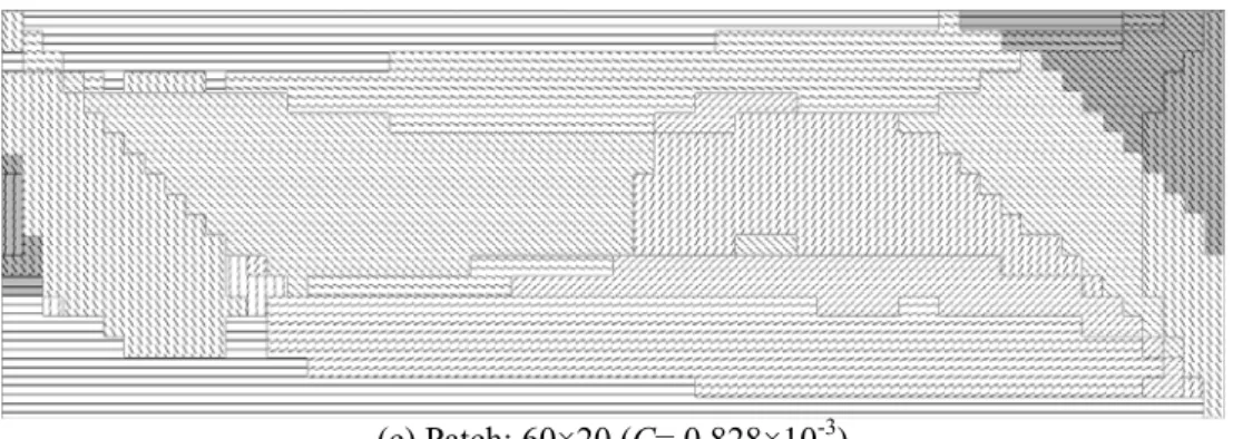
(c) Patch: 60×20 (C= 0.828×10⁻³)
Fig. 13 Optimization results using DC scheme (m=9)
For the problem shown in Fig. 13(c), 4 design variables are retained for each designable patch and totally 4800 design variables are used for the considered half structure with the BCP scheme. However, if the DMO scheme is adopted for the same problem, the number of design variables will be 10800. This comparison indicates clearly the benefit of the BCP scheme in the size reduction of the optimization problem.
The ability of the BCP scheme is further tested by means of the following numerical example of 36 orientations (m=36). In this test, 6 design variables (mv=6) are needed in each designable patch. In contrast, the DMO scheme needs mv=36 which is six times more. As shown in Fig. 14, a reasonable layout of the orientations is achieved by means of the BCP scheme.
Fig. 14 Optimization results using BCP scheme (Patch: 12×4, m=36)
5. Discussions
In this section, the influences of the bi-value coding and initial weights upon the optimization results are discussed. It should be noticed that there exist some other choices for the coding of candidate materials in the BCP scheme apart from those listed above. One alterative rule for sjk is expressed as
1
2
1
2
jkistep
imod
s
istep
imod
⎧
>
⎪⎪
= ⎨
⎪−
≤
⎪⎩
(15) with2
0
0
kistep
j
j
j
istep
j
istep
istep
istep
imod
j
istep
j
istep
istep
=
⎧
⎢
⎥
⎢
⎥
−
×
−
×
≠
⎪
⎢
⎥
⎢
⎥
⎪
⎣
⎦
⎣
⎦
= ⎨
⎢
⎥
⎪
−
×
=
⎢
⎥
⎪
⎣
⎦
⎩
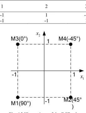
(16)For instance, the alternative coding is listed in Table 6 for mv=2 and the illustration is shown
in Fig. 15. Compared with the coding given in Table 1, the positions of material 3 and 4 are exchanged.
Table 6 Alternative codes for
s
jkvalues (mv=2, m=16) j k 1 2 3 4 1 -1 1 -1 1 2 -1 -1 1 1M1(90°)
M2(45°
)
M4(-45°)
M3(0°)
1x
2x
-1
-1
1
1
Fig. 15 Illustrations of the BCP scheme
The optimization results of two tests are shown in Fig. 16. Compared with the layouts given in Fig. 6(c) and Fig. 12(a), the current solutions using codes specified in Table 6 are a little better and the corresponding orientation layouts are slightly different. For the optimization result shown in Fig. 16(a), the direction of the principal stress is plotted. It is seen that with the set of discrete orientations, the optimal orientation in each patch globally agrees with the principal stress direction but the local difference does exist.
Optimization results Principal stress direction (a) Square plate under vertical force m=4 (C=1.162×10⁻⁴)
(b) Simply-supported beam m=4 Patch:12×4 (C= 0.845×10⁻³) Fig. 16 Optimization results using codes in Table 6
In fact, more possibilities of the bi-value coding exist in the case of large number of candidate materials and it is hard to test all of them. Even this is done numerically, we cannot ensure which choice may lead to the global optimum because the widely used sequential convex programming (SCP) lacks the ability to seek the global optimum for complicated non-monotonous problem. Besides, the optimization problem may not be a convex problem itself. For example, the considered objective function defined by the structural compliance is usually non-monotonous and non-convex for the considered design variables related to the discrete orientations. Nevertheless, numerical tests indicate that the bi-value coding is able to yield reasonable optimization results although the global optimum solution is not ensured.
As to the initial weights, a uniform value is adopted in all above tests as in the UMMI schemes presented in [12, 14]. It means that the initial value of each design variable is set to be
xij=0 for each designable element or area. Geometrically, it corresponds to the origin of the bi-value coding scheme illustrated in Fig. 1 and Fig. 17. Now, non-uniform initial weights are tested to illustrate their influences. Take still the square plate under vertical force as an example. 4 orientations coded in Table 6 are adopted. If the initial values of design variables are set to be
xij=0.5, it is known from Fig. Fig. 15 that the material M4 with the orientation of -45° is preferably selected by the non-uniform initial weights. The corresponding layout solution is shown in Fig. 18 (a). Likewise, if the initial values of design variables are set to be xij=-0.5, the material M1 with the orientation of 90° is preferably selected according to Fig. 17(b). Obviously, the comparison of the compliance values indicate that both solutions resulting from non-uniform initial weights are worse than that presented in Fig. 16(a). It is therefore preferable to use uniform initial weights at the beginning of the optimization process.
(a) xij=0.5 (≈-45°)
C=2.445×10⁻⁴
(b) xij=-0.5 (≈90°)
C=1.663×10⁻⁴
Fig. 18 Influences of initial weights upon final orientations
6. Conclusions
A new parameterization scheme named BCP is proposed in this work to deal with the layout design of discrete material orientations for laminate composite. The theoretical expression of the BCP is constructed in an explicit way for any number of materials. As the involved number of design variables depends upon the number of materials in logarithmic form, it is therefore advantageous over the exiting DMO and SFP schemes to deal with large-scale problems.
Numerical examples show that the BCP scheme can produce a stable convergence and the solution can easily be achieved with up to 36 material orientations. Furthermore, from the tests of the initial values of design variables, it concludes that the uniform initial weights with xij=0 are preferably selected in BCP to give rise to a satisfactory solution. As an extension of the current work, it is believed that the BCP will open its proper applications in the practical design of composite structures with a variety of objective functions and constraints in the future.
Acknowledgement
This work is supported by the National Natural Science Foundation of China (10925212, 90916027) and the Walloon Region of Belgium and SKYWIN (Aerospace Cluster of Wallonia) through the project VIRTUALCOMP (Contract RW-6293).
References
[1] R. Le Riche, R.T. Haftka, Improved genetic algorithm for minimum thickness composite laminate design, Composites Engineering, 5 (1995) 143-161.
[2] S. Adali, A. Richter, V.E. Verijenko, E.B. Summers, Optimal design of hybrid laminates with discrete ply angles for maximum buckling load and minimum cost, Composite Structures, 32 (1995) 409-415.
[3] A. Todoroki, R.T. Haftka, Stacking sequence optimization by a genetic algorithm with a new recessive gene like repair strategy, Composites Part B: Engineering, 29 (1998) 277-285.
[4] J. Thomsen, Topology Optimization of Structures Composed of One or 2 Materials, Struct Optimization, 5 (1992) 108-115.
[5] O. Sigmund, S. Torquato, Design of materials with extreme thermal expansion using a three-phase topology optimization method, Journal of the Mechanics and Physics of Solids, 45 (1997) 1037-1067. [6] M.P. Bendsøe, O. Sigmund, Material interpolation schemes in topology optimization, Archive of Applied Mechanics, 69 (1999) 635-654.
[7] O. Sigmund, Design of multiphysics actuators using topology optimization - Part II: Two-material structures, Computer Methods in Applied Mechanics and Engineering, 190 (2001) 6605-6627.
[8] L. Yin, G.K. Ananthasuresh, Topology optimization of compliant mechanisms with multiple materials using a peak function material interpolation scheme, Structural and Multidisciplinary Optimization, 23 (2001) 49-62.
[9] D.Y. Jung, H.C. Gea, Design of an energy-absorbing structure using topology optimization with a multimaterial model, Struct Multidiscip O, 32 (2006) 251-257.
[10] Y.L. Mei, X.M. Wang, A level set method for structural topology optimization with multi-constraints and multi-materials, Acta Mech Sinica, 20 (2004) 507-518.
[11] E. Lund, J. Stegmann, On structural optimization of composite shell structures using a discrete constitutive parametrization, Wind Energy, 8 (2005) 109-124.
[12] J. Stegmann, E. Lund, Discrete material optimization of general composite shell structures, International Journal for Numerical Methods in Engineering, 62 (2005) 2009-2027.
[13] E. Lund, Buckling topology optimization of laminated multi-material composite shell structures, Composite Structures, 91 (2009) 158-167.
[14] M. Bruyneel, SFP - a new parameterization based on shape functions for optimal material selection: application to conventional composite plies, Structural and Multidisciplinary Optimization, (2010).
[15] P. Pedersen, On optimal orientation of orthotropic materials, Structural and Multidisciplinary Optimization, 1 (1989) 101-106.
[16] P. Pedersen, Bounds on elastic energy in solids of orthotropic materials, Structural and Multidisciplinary Optimization, 2 (1990) 55-63.
[17] H.C. Gea, J.H. Luo, On the stress-based and strain-based methods for predicting optimal orientation of orthotropic materials, Structural and Multidisciplinary Optimization, 26 (2004) 229-234. [18] A.R. Díaz, M.P. Bendsøe, Shape optimization of structures for multiple loading conditions using a homogenization method, Structural and Multidisciplinary Optimization, 4 (1992) 17-22.
[19] H.C. Cheng, N. Kikuchi, Z.D. Ma, An improved approach for determining the optimal orientation of orthotropic material, Structural and Multidisciplinary Optimization, 8 (1994) 101-112.
[20] J. Stegmann, E. Lund, Discrete material optimization of general composite shell structures, Int J Numer Meth Eng, 62 (2005) 2009-2027.