Université de Montréal
Contributions of local, lateral and contextual habitat
variables to explaining variation in fisheries productivity
metrics in the littoral zone of a reservoir
par
Nathan Allen Satre
Département de sciences biologiques Faculté des arts et des sciences
Mémoire présentéà la Faculté des arts et des sciences en vue de l’obtention du grade de Maîtrise en sciences
en sciences biologiques
Novembre, 2015
Université de Montréal Faculté des arts et des sciences
Ce mémoire intitulé:
Contributions of local, lateral and contextual habitat variables to explaining variation in fisheries productivity metrics in the littoral zone of a reservoir
présenté par: Nathan Allen Satre
a été évalué par un jury composé des personnes suivantes:
Timothée Poisot Président-rapporteur Daniel Boisclair Directeur de recherche Pierre Legendre Codirecteur Jacques Brisson Membre du jury
Résumé
Puisque l’altération des habitats d’eau douce augmente, il devient critique d’identifier les composantes de l’habitat qui influencent les métriques de la productivité des pêcheries. Nous avons comparé la contribution relative de trois types de variables d’habitat à l’explication de la variance de métriques d’abondance, de biomasse et de richesse à l’aide de modèles d’habitat de poissons, et avons identifié les variables d’habitat les plus efficaces à expliquer ces variations. Au cours des étés 2012 et 2013, les communautés de poissons de 43 sites littoraux ont été échantillonnées dans le Lac du Bonnet, un réservoir dans le Sud-est du Manitoba (Canada). Sept scénarios d’échantillonnage, différant par l’engin de pêche, l’année et le moment de la journée, ont été utilisés pour estimer l’abondance, la biomasse et la richesse à chaque site, toutes espèces confondues. Trois types de variables d’habitat ont été évalués: des variables locales (à l’intérieur du site), des variables latérales (caractérisation de la berge) et des variables contextuelles (position relative à des attributs du paysage). Les variables d’habitat locales et contextuelles expliquaient en moyenne un total de 44 % (R2 ajusté) de la variation des métriques de la productivité des pêcheries, alors que les variables d’habitat latérales expliquaient seulement 2 % de la variation. Les variables les plus souvent significatives sont la couverture de macrophytes, la distance aux tributaires d’une largeur ≥ 50 m et la distance aux marais d’une superficie ≥ 100 000 m2, ce qui suggère que ces variables sont les plus efficaces à expliquer la variation des métriques de la productivité des pêcheries dans la zone littorale des réservoirs.
Mots-clés : modélisation de l’habitat des poissons, variables d’habitat, métriques de la
Abstract
As freshwater fisheries become increasingly prone to habitat alteration, it is critical we identify the components of habitat that greatly influence fisheries productivity metrics. Using fish habitat modeling, we compared relative contributions of three types of habitat variables to explain variation in abundance, biomass and richness metrics, and identified habitat variables most effective at explaining these variations. During the summers of 2012 and 2013, fish communities in 43 littoral sites were sampled from Lac du Bonnet, a reservoir in southeastern Manitoba (Canada). Seven different sampling scenarios, consisting of different sampling methods, years and time periods, were used to measure relative abundance, biomass and richness metrics for all species combined per site. Three types of habitat variables were measured: local (i.e. within site), lateral (i.e. shore characterization) and contextual (i.e. position relative to landscape attributes) variables. Together local and contextual habitat variables explained on average 44% R2adj of the variation across fisheries productivity metrics, while only 2% R2adj of the variation was explained by lateral habitat variables. Specifically, macrophyte coverage, distance to tributaries ≥ 50 m wide, and distance to marshes ≥ 100,000 m2 ranked most significant across metrics, suggesting these habitat variables may be most effective at explaining variation in fisheries productivity metrics in the littoral zone of reservoirs.
Keywords: fish habitat modeling, habitat variables, fisheries productivity metrics, reservoir,
Table of Contents
Résumé ... i
Abstract ... ii
Table of Contents ... iii
List of Tables ... iv List of Figures ... v List of Abbreviations ... vi Acknowledgements ... vii General Introduction ... 1 Preface... 1 Components ... 2 Habitat ... 2 Fisheries Productivity ... 4 Habitat Modeling ... 5 Author Contributions ... 7 Introduction ... 9
Materials and Methods ... 11
Study Area ... 11 Data Collection ... 13 Analyses ... 17 Results ... 19 Discussion ... 23 General Conclusion ... 26 References ... 28 Appendix ... 33
List of Tables
Table I: Habitat variables used to explain variation in FPM and their potential effects. * denotes variable was log10 transformed to improve distribution normality. Bold face indicates variables retained in habitat variable pre-selection. ... 16 Table II: Variable type assessment results for the reduced set of fish datasets. Displayed are R2adj values corresponding to the percentage of variation uniquely explained by each habitat dataset or their intersections (∩) for a given fish dataset. Bold face indicates statistical significance for testable fractions (local, lateral and contextual only). ... 20 Table III: Key variable assessment results for the reduced set of fish datasets. “X” denotes statistical and biological significance of a habitat variable explaining variation within a given fish dataset in at least one forward selection. Percent row indicates the percentage of fish datasets for which a variable was selected at least one time. ... 22
List of Figures
Figure 1: Flowchart detailing an example of the fish habitat modeling process. ... 6 Figure 2: Map detailing the 43 sampling sites established in the littoral zone of Lac du Bonnet and the reservoir’s geographic position within Canada. ... 12
List of Abbreviations
Bio.: biomass Dist.: distance
Ed: boat electrofishing, day-time hours in 2012 En: boat electrofishing, night-time hours in 2012 FPM: fisheries productivity metrics
Gd: gillnetting, day-time hours in 2012 Lat.: lateral
NSERC: Natural Sciences and Engineering Research Council of Canada P/A: presence or absence
r: correlation coefficient
R2: coefficient of determination
R2adj: adjusted coefficient of determination SD: standard deviation
Sd1: seining, day-time hours in 2012 Sd2: seining, day-time hours in 2013 Sd3: seining, day-time hours in 2013 Sn: seining, night-time hours in 2013 sub.: substrate
Acknowledgements
Thank you to Guillaume Bourque, Daniel Boisclair and Pierre Legendre for their support of me and this project. Thank you to Jean-Michel Matte, Suzie Dubuc, Mathias Quiniou (Université de Montréal), Mark Lowdon (AAE Tech Services Inc.) and Doug Watkinson (Fisheries and Oceans Canada, Winnipeg) for their work in the field. Thanks also to Joel Hunt, Gary Swanson (Manitoba Hydro), Doug Leroux and Ken Kansas (Manitoba Conservation and Water Stewardship) for their logistical support. Additional supporters include Jean-Martin Chamberland, Laura Wheeland, Riley Pollom, the NSERC HydroNet Administrative Centre and members of the Boisclair Lab at Université de Montréal. Financial support was provided by an NSERC Collaborative Research and Development Grant, Manitoba Hydro, Manitoba Conservation and Water Stewardship, Fisheries and Oceans Canada and North/South Consultants Inc.
General Introduction
Preface
As human population continues to increase, so does the quantity of resources needed to sustain a growing population. Some of these basic resources include food, water and shelter (Denton 1990), which can be found throughout the landscape or are products of resources found there. A growing population requiring more resources also requires exploiting more of the landscape from which these resources are derived. Caveats of exploitation include potential side effects to the environment and organisms which occupy it; in many cases these side effects are not well understood.
Research on this expansive topic is necessary to develop resources sustainably. However research should be focused enough that conclusions are informative and readily utilized by government and industry, groups actively involved in resource development. The research described here focuses on water resources and the habitat variables within them, which can be used to explain variation in fisheries productivity metrics. The research here allows us to recognize components of habitat found in water resources that may influence fish abundance, biomass and richness, which is increasingly important as water resources continue to be developed across the globe.
Understanding which components of habitat explain variation in fisheries productivity metrics is important so proper mitigation, compensation or prevention steps can be implemented to ensure the productive capacity of water resources are not diminished. This is an important consideration considering nearly one billion people rely on fish as their primary source of animal protein, especially in developing nations (WHO/FAO Joint Expert Consultation 2003). In developed nations like Canada, no net loss of productivity of fish habitat is a guiding principle for habitat management (Minns 1997) and a major factor in water resource development (e.g. hydroelectric generation), however means of achieving no net loss is not always clear.
We hope that the findings of our study shed light on the important components of habitat influencing fisheries productivity, and therefore inspire innovative ways to maintain fisheries productivity in light of resource development.
Components
Habitat
Habitat can be defined as a physical space occupied or not by an organism (Odum 1971) during a certain life stage at a given time (Begon et al. 1990), allowing or potentially allowing an organism to perform at least one vital function (e.g. survival, growth, reproduction). These vital functions are dependent upon habitats comprised of many variables (i.e. measurable environmental traits) that favour the vitality of an organism. These habitat variables reflect natural constraints on productivity (Yasué and Dearden 2006) and have consequentially been used to evaluate it.
As human population continues to increase, so does the conversion of natural habitats; in doing so these habitats become degraded, threatening biodiversity and the benefits we derive from it (Hoekstra et al. 2005). Habitat loss or alteration affects productivity, threatening the survival of fish (Evans et al. 1996) and other aquatic organisms (Richter et al. 1997). Specifically, degraded habitats have restructured biotic communities and diminished diversity and productivity (Wang et al. 2001). But what components of habitat influence productivity; are they variables that can be measured locally or more broadly, can they be measured at all? This is the fundamental question of this study, and answers will provide insight into how losses in fisheries productivity can be mitigated, compensated or prevented. With this understanding we can begin to avoid components of habitat that when altered, equate to losses in fisheries productivity.
Variables found within a site (e.g. macrophytes, substrate), otherwise known as local habitat variables, have long been front and centre of efforts to increase fisheries productivity, and for good reason. The importance of submerged macrophytes to the diversity, distribution, abundance and productivity of northern temperate fish has been indicated by many researchers (e.g. Weaver et al. 1997). Macrophytes may also provide cover from predators (Savino and
Stein 1982) and increased densities of macroinvertebrates (Crowder and Cooper 1982), a source of food. For some fish assemblages, open and rocky habitats are preferred (Stang and Hubert 1984, Weaver et al. 1997) suggesting substrate may play a role in productivity. Wang et al. (2006) support this suggestion claiming substrate particles strongly influence fish assemblages. Randall et al. (1996) developed a relationship between an index of fish production and habitat features which included submerged macrophytes. Their project sought to test the relationship between macrophyte density and species richness, fish size, density and biomass. In their study, fish production was measured indirectly using a production index estimated from measures of fish biomass and size. As a result, their production index positively correlated with macrophyte density and species richness, and negatively correlated with slope. Another question was to determine if the index could be predicted from macrophyte density and other habitat variables which included slope, wind exposure, effective fetch, substrate composition and phosphorus concentration. Stepwise multiple regression indicated that macrophyte density, species richness and phosphorus best predicted the production index.
Another project of interest focusing on local habitat variables includes Pratt and Smokorowski (2003). An objective of their study was to determine the summer day-time habitat use of fish in the littoral zone of a north temperate mesotrophic lake, among habitat types based on differences in substrate, macrophyte cover and depth. Measures of fish abundance, richness and diversity were compared across multiple habitat types using a method of rapid visual underwater assessment. Multivariate analyses indicated most species were associated with macrophytes; however some were primarily associated with rocky substrate (Pratt and Smokorowski 2003). Shallow mud habitats that contained no structure were found to contain significantly fewer species and diversity than all other habitat types. Two main assemblages of fish were identified in their study; Logperch (Percina caprodes) and Smallmouth bass (Micropterus dolomieu) characterized the shallow rock fish assemblage, whereas the remaining species found in the system were primarily associated with vegetated habitats (Pratt and Smokorowski 2003).
These studies highlight the importance of local habitat variables on various fisheries productivity metrics (FPM) and suggest these variables may play an important role explaining
variation in FPM. However local habitat variables are not the only variables worth considering; what about variables and ecological processes operating at a larger spatial scale? Fortin et al. (2002) refer to ecological processes and how they often operate on multiple spatial scales. Brind'Amour et al. (2005) similarly state that interactions between littoral fish communities and their habitat occur at multiple spatial scales, therefore habitat variables observable at different spatial scales may influence fish community structure. While many studies have focused on local habitat variables, others have shown it may be more important to use habitat variables from a spatially larger scale, specifically for developing fish habitat models (Kruse et al. 1997, Nelson et al. 1992, Rieman and McIntyre 1995).
Studies similar to ours (i.e. Bouchard and Boisclair 2008, Wang et al. 2003) have incorporated habitat variables from fine to broad spatial scales. Both studies included variables measured from local, lateral (i.e. shore characterization) and contextual (i.e. position relative to landscape attributes) scales, fine to broad respectively. Lateral habitat variables, for instance trees, have been cited as an important driver of fish abundance in streams (Inoue and Nakano 2001). Roads, another lateral variable, have been associated with neagative effects on biotoic integrity in aquatic ecosystems (Trombulak and Frissell 2000). Contextual habitat variables, for instance distance (m) to marshes, have been cited as providing spawning and nursery habiat for a fish community (Wei et al. 2004). Distance (m) to tributaries, another contextual variable, defines proximity to complementary resources such as thermal refuge or alternate food source (Bruns et al. 1984), (Dunning et al. 1992). These are just a few examples of habitat variables measured more broadly that may also influence FPM.
Fisheries Productivity
Fisheries productivity can be measured in different ways either directly or indirectly. By definition, annual production is the generation of tissue weight per unit area (e.g. kg per hectare) in the course of a year, and is determined by the rate of reproduction, rate of growth and the rate of mortality (Murphy and Willis 1996). Indirectly productivity can be monitored by observing baseline changes in various fisheries productivity metrics which may include abundance, biomass and richness. For the purposes of this study we are concerned with
differences in FPM among different habitats (sites sampled) as opposed to changes in productivity over time.
Abundance is defined here as the number of individuals divided by effort; this metric can produce an estimate of individuals present within a system. Significant differences in fish abundance from habitat to habitat (or sampling site to site) may indicate a habitat and its variables are more productive than other habitats. Biomass is defined here as grams divided by effort; this metric can produce an estimate of weight or biomass of individuals within a system. Significant differences in fish biomass from habitat to habitat may also indicate more productive habitats, however body condition, a measure of physical health can also be observed. Furthermore, these metrics can be used to estimate total abundance or biomass of a system, or be broken down to describe specific species and size-classes. Richness is another metric that can be used to measure fisheries productivity, and is frequently used as a measure of overall system health (Harris and Silveira 1999). Richness is defined here as the number of species per sampling event, and can produce an estimate of the number of species present in a system.
Using a combination of metrics we will be better equipped to capture variation in productivity influenced by habitat variables. Wang et al. (2003) and Bouchard and Boisclair (2008) used similar metrics in their studies to attribute variation in FPM to spatial scales and habitat variables. In key findings of both studies, variation in abundance was best explained using local habitat variables.
Habitat Modeling
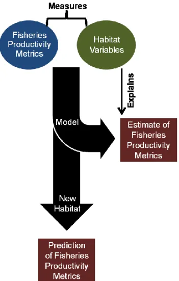
Measures of habitat variables and fisheries productivity metrics will be used to produce fish habitat models (Figure 1). These models will be used to provide estimates of FPM explained by habitat variables, and may also be used to predict FPM when applied to new habitat (e.g. sampling site, lake). Using these models, functional relationships between species and habitat can be detected (Guisan and Zimmermann 2000). Here, fish habitat modeling will detect relationships between FPM and habitat to help identify productive habitat variables and those variable types (i.e. local, lateral and contextual).
Figure 1: Flowchart detailing an example of the fish habitat modeling process.
Fish habitat models provide an invaluable tool to researchers and managers by providing the ability to forecast fine- and broad-scale effects of habitat modification on fish populations and communities (Olden and Jackson 2001). The ability to forecast these effects are crucial to ensuring fisheries productivity is not diminished. However a major challenge to developing fish habitat models lies in their transferability from system to system, largely because most models are based on local habitat variables (Wall et al. 2004). In order to increase transferability, habitat variables from broader spatial scales should be incorporated into fish habitat models. These broad-scale models are necessary as watershed management has become a common fish conservation approach (Wall et al. 2004).
Recently numerous studies have employed fish habitat modeling as a tool to estimate and predict fish distributions (e.g. Porter et al. 2000, Wall et al. 2004) or estimate and predict abundance (e.g. Bouchard and Boisclair 2008, Inoue and Nakano 2001, Reyjol et al. 2008). Frequently these studies are the focus of rivers and streams and have used explanatory variables from multiple spatial scales to construct their models. Often these studies are species-specific or in response to SARA (Species at Risk Act) or ESA (Endangered Species Act) listings. Other studies have focused on single or multiple lakes (e.g. Cvetkovic et al. 2009, Pratt and Smokorowski 2003, Randall et al. 1998) to build fish habitat models as a management tool.
Despite the variations in which these studies were carried out, much can be learned and applied to the study presented here. As such, many of the above citations were used to build methodology, guide analysis and support results and conclusions. One clear take away from this literature review is the importance of local habitat variables in developing fish habitat relationships; with this in mind, we can only hypothesize this will remain consistent in our findings.
Author Contributions
The research described here was a result of contributions from Nathan Allen Satre, Guillaume Bourque, Daniel Boisclair and Pierre Legendre. Goals and objectives of this project were developed by Daniel Boisclair, in addition to funding, advising and editorial support. In charge of logistics and advising was Guillaume Bourque. Guillaume also played an important role in the data collection process, statistical advising and editorial support. We the authors credit him greatly for the success of this project. Pierre Legendre provided critical support in the area of statistical advising and also served on the project review committee. We also thank him for his editorial support.
Nathan joined this project as a M.Sc. candidate in May 2012, and was tasked with the ownership of two project objectives, one of which is presented in this mémoire. He was responsible for planning how these objectives would be carried out, the execution process and reporting the findings. From day one, Nathan was invested in developing protocol for how the data collection process would proceed. Guillaume and Nathan implemented two field seasons
in 2012 and 2013 in which the majority of data collection took place. In preparation for data analysis, Nathan enrolled in BIO 6077 (Analyse quantitative des données biologiques) to better understand the methods available for analysis, and attended workshops demonstrating the software that would be used for analysis. Nathan and Guillaume shared a role in the analysis process and were advised by Pierre Legendre. Reporting was primarily the responsibility of Nathan, whose works includes this mémoire, a manuscript (in revision), contributions to a CSAS report, and multiple presentations and press releases.
Introduction
Habitat can be defined as a physical space occupied or not by an organism (Odum 1971) during a certain life stage at a given time (Begon et al. 1990), allowing or potentially allowing an organism to perform at least one vital function (e.g. survival, growth, reproduction). The location, shape and size of a habitat may vary in physical space or time (Southwood 1977) according to abiotic and biotic conditions (Odum 1971).
The physical space constituting a habitat can be viewed from a continuum of spatial scales (Morrison et al. 2012). Ecological processes often operate on multiple spatial scales (Fortin et al. 2002) which can range from broad (e.g. 200-20000 m) to fine (e.g. 0.2-200 m) in extent, structuring the habitat organisms occupy. Understanding these ecological processes, the spatial scales of habitat at which they operate, and how they influence communities is central in spatial analysis.
Habitat models are tools that can be used to better understand these processes. With these tools, ecological theory, data (response and explanatory variables), and statistical methods are combined to create models based on correlations (Austin 2002). Using these models, functional relationships between species and habitat can be detected (Guisan and Zimmermann 2000). For instance, modeling can produce estimates and predictions of species abundance given the explanatory power of habitat variables or forecast changes in abundance given simulated habitat modifications.
Over time, freshwater systems have sustained habitat loss or alteration as a result of anthropogenic activities. The side effects of such activities have been documented throughout scientific literature and continue to be explored to date. While habitat loss or alteration affects productivity, threatening the survival of fish (Evans et al. 1996) and other aquatic organisms (Richter et al. 1997), much less is known about which particular habitat variables relate to productivity.
In general, littoral-based fish habitat models have focused largely on relationships between fisheries productivity metrics (e.g. abundance, biomass and richness) and local habitat variables (i.e. within site) (e.g. Bryan and Scarnecchia 1992, Gamboa-Pérez and Schmitter-Soto 1999). However, some studies suggest using contextual habitat variables (i.e.
position relative to landscape attributes; e.g. Table I) to explain and predict fish distribution over local habitat variables (Porter et al. 2000). Other studies have suggested and used several types of habitat variables. Brind'Amour et al. (2005) state that interactions between littoral fish communities and their habitat occur at multiple spatial scales, therefore habitat variables observable at different spatial scales may influence fish community structure. In their study, Brind'Amour et al. (2005) used multiple spatial scales (broad to fine) to quantify relationships between fish community descriptors and habitat variables present in a Québec (Canada) lake. Similarly, Bouchard and Boisclair (2008) examined multiple spatial scales to quantify the relative importance of habitat variables on the density of a Québec river species. In another case, Wang et al. (2003) identified key habitat variables that explained stream fish assemblage patterns in 79 U.S. watersheds by incorporating habitat variables from multiple spatial scales in the modeling process. Together these studies share a common approach requiring the use of modeling, measures of fisheries productivity metrics (FPM), and several types of habitat variables with the goal of detecting functional relationships between species and their habitat.
Local, lateral (i.e. shore characterization) and contextual habitat variables are three different types of habitat variables encompassing variables present within a sampling site to variables that span an entire study area. As noted, similar studies have focused on using several types of habitat variables to explain variation in FPM in rivers and lakes; however few, if any, have used this modeling approach in reservoirs, systems in which a high degree of habitat alteration has already occurred.
The objectives of this study are (i) to compare relative contributions of local, lateral and contextual habitat variables to explain variation in fish abundance, biomass and richness metrics in the littoral zone of a reservoir (ii) and to identify habitat variables most effective at explaining these variations.
Materials and Methods
Study Area
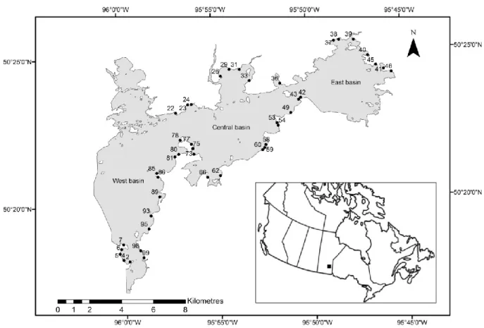
Sampling was performed throughout Lac du Bonnet, Manitoba (Canada); a 115 km2 hydroelectric reservoir situated between the interior plains and Canadian Shield. This reservoir, formed circa 1951 by damming of the Winnipeg River, can be characterized as turbid, mesotrophic and windswept with a mean depth of 7.7 m. Lac du Bonnet can be divided into three basins from west to east: the west basin includes the main channel (Winnipeg River) and can be defined as lotic; the central and east basins can be defined as lentic (Figure 2). Lac du Bonnet was an exceptional study area based upon the objectives of this study for two primary reasons: (i) its position between the interior plains and Canadian Shield, allowing a diversity of habitat to be sampled; (ii) its lotic and lentic properties, allowing us to extend our comparisons to rivers and lakes.
Figure 2: Map detailing the 43 sampling sites established in the littoral zone of Lac du Bonnet and the reservoir’s geographic position within Canada.
Data Collection
Seven fish sampling scenarios, consisting of different sampling methods (seining, boat electrofishing and gillnetting), years (2012 and 2013) and time periods (day and night) were used to estimate three fisheries productivity metrics (abundance, biomass and richness) in 43 sampling sites. (The use of all sampling methods in both years and time periods was unfeasible due to time and resource constraints.) Sampling sites were established in the littoral zone (Figure 2), defined here as the area between the 0 and 3 m isobaths. Each site measured 200 m in length (parallel to shore) to accommodate all gears without overlap. Fish sampling spanned the months of July-August 2012 and 2013.
Fish sampling methods included seining, boat electrofishing and gillnetting. Seining was selected as a common method used to sample fish in the littoral zone (Pierce et al. 1990); it also allows precise estimation of volume or surface area that surpasses many other gears used in this zone (Brind'Amour and Boisclair 2004). Boat electrofishing and gillnetting were selected based on their history of successful use in Lac du Bonnet by provincial and federal agencies. Multiple sampling methods were selected as no single method can provide a complete quantitative description of fish community structure in littoral zone of lakes (Weaver et al. 1993). Each sampling scenario was completed by a single team in 2012 or 2013 during day-time (2.5 hours after sunrise to 2.5 hours before sunset) or night-time periods (end of evening nautical twilight to start of morning nautical twilight). In 2012 seining (Sd1), boat electrofishing (Ed) and gillnetting (Gd) were performed during day-time hours in all 43 sites. In 2013 seining was performed twice (Sd2, Sd3) in all 43 sites during day-time hours; during night-time hours, seining (Sn) was performed in 30 sites and boat electrofishing (En) was performed in 43. Seining was performed using a 35 m long by 1.5-3 m wide ½” mesh beach seine in depths ranging between 0.5-1.1 m minimum depth to 1.5-3 m maximum depth. Seine hauls averaged 157 m2 (SD = 19.7 m2) and effort was normalized to 100 m2 for analysis. Boat electrofishing was performed using a Smith-Root SR20 electrofishing boat equipped with a 5.0 GPP electrofisher. Transects of 100 m were shocked parallel to shore in depths ranging between 1-1.5 m (median depth of littoral zone) for an average of 277 shocking seconds (SD = 63 shocking seconds), effort normalized to 100 shocking seconds. Gillnetting was performed
using 5/8”, 1” (monofilament), 2”, 3” and 4 ¼” (multifilament) mesh gillnets. These five mesh sizes were used to create four 20 m by 1.8 m nets which were set simultaneously at a 45° angle between the 2 m and 3 m isobaths ± 0.5 m. Average fishing time was 1 hour and 33 minutes (SD = 7 minutes), effort normalized to 1 hour.
During these sampling events, species, total length, and weight (at least 30 individuals per species) were recorded for fish captured. Species length-mass relationships were developed from weighed individuals to assign a weight to all fish captured. All species were combined to produce one value of relative abundance (# individuals / effort), biomass (g / effort) and richness (# species / sampling event) per scenario per site.
Habitat variables were selected because of their potential effects on FPM (Table I). Local habitat sampling was conducted once per site in late August and early September 2012. Slope (%) was measured from the 3 m isobath to the shoreline 5 times, dividing 3 m by the mean distance from shore. Macrophyte coverage (%) and substrate composition (%) were estimated visually and tactilely 10 times within a site using a 50 by 50 cm quadrate in a stratified random sampling design, stratified by depth zones (0-1 m, 1-2 m, 2-3 m). Substrate composition was classified using four substrate variables, which consisted of different substrate types used by Senay et al. (2014). Compacted fine substrate consisted of clay substrate type in compacted form. Loose fine substrate consisted of a combination of clay, silt and sand substrate types. Small coarse substrate consisted of a combination of gravel and pebble substrate types. Large coarse substrate consisted of cobble to boulder substrate types. Mean depth (m) was measured using a weighted average of the median depth of each depth zone (i.e. 0.5 m, 1.5 m, 2.5 m) weighted by the proportion of each depth zone in the site.
Measures of lateral habitat variables (Table I) were compiled for each site using the most recent satellite imagery available in Google Earth 7.1 (2007). Variables included either presence or absence (P/A) of bog, grassland, road or golf course occupying the shore parallel to the site.
Measures of contextual habitat variables (Table I) were complied for each site using ArcGIS 10.2 (ESRI 2013) or Google Earth 7.1 (2007). Distances (m) to large, permanent and all tributaries, large and all marshes, artificial reef and main channel were measured using a
minimum in-water trajectory. Large tributaries were defined as those ≥ 50 m in width prior to the river delta. Permanent tributaries included large tributaries and others with a consistent seasonal flow into the reservoir. All tributaries included big and permanent tributaries and any intermittent tributaries visible using satellite imagery. Large marshes were defined as those ≥ 100,000 m2 in surface area, consisting of dense macrophyte beds through which navigation was difficult. All marshes included large marshes and others ≥ 10,000 m2 in surface area (marshes < 10,000 m2 were not included). Artificial reef was defined as the area of boulders protruding from open water extending ~90 linear m in the central basin. Main channel was defined as the deepest portion of the Winnipeg River channel situated in the west basin. Average fetch was defined as the maximum distance (km) waves can travel without obstruction given a mean wind angle of 286°. This angle was computed as the circular mean hourly wind direction using data from May to November 2012 by Environment Canada (2013) at Pinawa weather station. West basin and east basin were denoted in a binary fashion: 1 if the site was located in the respective basin, 0 otherwise (Figure 2). Northwest shore was defined as the shoreline occupying the north and west shores of Lac du Bonnet and was also denoted in a binary fashion (Figure 2).
Table I: Habitat variables used to explain variation in FPM and their potential effects. * denotes variable was log10 transformed to improve distribution normality. Bold face indicates variables retained in habitat variable pre-selection.
Type Habitat variable Unit Potential effects Reference(s)
L
ocal
Slope % Influences biomass of submerged macrophyte communities
(Duarte and Kalff 1986)
Macrophyte
coverage % Productive feeding environment; refuge from predators; reproductive environment for phytophilic fish species
(Randall et al. 1996) (Bolding et al. 2004) (Dibble et al. 1997) Su bs tr
ate Compacted fine Loose fine % % Substrate particles strongly influence fish assemblages (Wang et al. 2006)
Small coarse* %
Large coarse* %
Mean depth m Among most important variables in explaining variability in relative fish biomass in Argentina lakes and reservoirs
(Quiros 1990)
L
ater
al
Bog P/A Low pH often cited as limiting fish
species richness (Rahel 1984)
Grassland P/A Presence or absence of trees cited as important driver of fish abundance in streams
(Inoue and Nakano 2001)
Road P/A Associated with negative effects on biotic integrity in aquatic ecosystems
(Trombulak and Frissell 2000) Golf course P/A Associated with heavy pesticide and
fertilizer use that may pollute runoff (Watschke et al. 1989)
C on tex tu al Dis tan ce to
Large tributaries m Defines the proximity to complementary resources such as
thermal refuge or alternate food source
(Bruns et al. 1984) (Dunning et al. 1992) Permanent tributaries m All tributaries m
Large marshes m Used preferentially for spawning and nursery habitat by the majority of the Great Lakes fish community
(Wei et al. 2004)
All marshes m
Artificial reef m Area of increased habitat heterogeneity
may favour increased species richness (Guegan et al. 1998) Main channel m Fish communities are linked to flow
regimes (Pegg and Pierce 2002)
Average fetch km Significant predictor of physical habitat conditions and fish abundance in the Great Lakes; significant predictor of biomass for three Great Lakes fish species (Randall et al. 1996) (Randall et al. 1998) (Randall et al. 2004) Geo gr ap hical class if icatio
n West basin East basin P/A P/A Lotic to lentic transition observed in basins moving west to east
Northwest shore P/A Contrast in local habitat composition and fish community observed among northwest and southeast shores, presumably a factor of fetch exposure (mean wind angle 286°)
Analyses
Twenty-one univariate fish datasets (all species combined), specific for each sampling scenario, were formed detailing relative abundance, biomass or richness metrics per site (Appendix I). Relative abundance and biomass metrics were normalized for effort and log10 transformed to improve distribution normality. Three multivariate habitat datasets were formed detailing local, lateral or contextual habitat variables per site. All habitat variables were standardized (mean of 0 and a standard deviation of 1) (using decostand function of the vegan (Oksanen et al. 2012) package in R (R Core Team 2012)), giving each variable the same spread and weight.
Habitat variable pre-selection was performed to identify variables significantly correlated with at least one fish dataset. This was achieved by running a multiple linear regression (using rda function of the vegan package in R) on each pair of 21 fish datasets and 3 habitat datasets, then testing the relationship of each pair for significance (≤ 0.05 p-value) using a permutation test for redundancy analysis (anova.cca function of the vegan package in R, 9999 permutations). Provided a significant relationship, a forward selection (forward.sel function of the packfor (Dray et al. 2011) package in R) was run on each pair, identifying significant habitat variables that explained ≥ 10% R2 of the variation for any fish dataset. This process was repeated up to three times per pair, each time removing the variable of greatest significance as to increase the likelihood of other variables being identified as significant. The combination of these selected habitat variables formed a reduced set of habitat variables, having shown a statistically (≤ 0.05 p-value) and biologically (≥ 10% R2) significant correlation with at least one fish dataset.
Fish dataset pre-selection was performed to identify fish datasets significantly correlated with the reduced set of habitat variables. This was achieved by running a multiple linear regression on each pair of 21 fish datasets and the reduced set of habitat variables, then testing the relationship of each pair for significance. Fish datasets exhibiting a significant relationship with the reduced set of habitat variables formed a reduced set of fish datasets.
Variable type assessment consisted of apportioning the variation (R2adj) of the reduced set of fish datasets among the 3 types of habitat variables within the reduced set of habitat
variables using variation partitioning developed by Borcard et al. (1992) (varpart function of the vegan package in R). Variation of abundance, biomass or richness metrics in reduced fish datasets were apportioned into mutually exclusive partitions, i.e. local, lateral, contextual, their intersections or unexplained. Local, lateral and contextual partitions were tested for significance using partial linear regression (rda function of the vegan package in R) and permutation test for redundancy analysis. Local, lateral and contextual partitions were compared based on average variation explained (R2adj) and based on the number of fish datasets for which these partitions were significant.
Key variable assessment identified habitat variables (from the reduced set) most effective at explaining variation in the reduced set of fish datasets. This was achieved by running a forward selection on each pair of reduced fish datasets and reduced set of habitat variables, identifying significant variables that explained ≥ 10% R2 of the variation for the respective fish dataset. This process was repeated up to three times per pair using the same criteria used in habitat variable pre-selection. Habitat variables were compared based on the number of fish datasets for which these variables were identified as significant.
Results
In habitat variable pre-selection 12 out of 22 habitat variables were retained, having shown a statistically and biologically significant correlation with at least one fish dataset. The reduced set of habitat variables consisted of slope, macrophyte coverage, compacted fine and loose fine substrate (four local habitat variables), grassland (one lateral habitat variable), distance to large tributaries, distance to permanent tributaries, distance to large marshes, distance to artificial reef, average fetch, east basin and northwest shore (seven contextual habitat variables). This process nearly reduced the number of explanatory habitat variables by half, resulting in a more parsimonious set of habitat variables used to explain variation in FPM.
In fish dataset pre-selection 12 out of 21 fish datasets were retained, having exhibited significant correlation with the reduced set of habitat variables. The reduced set of fish datasets consisted of six datasets estimating abundance, one estimating biomass and five estimating richness across a series of sampling scenarios (Table II). Having removed fish datasets with non-significant correlations, assessments of variable type and key variables could proceed.
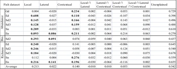
In variable type assessment, local habitat variables uniquely explained on average 21% (R2adj) of the variation within the 12 reduced fish datasets, while lateral and contextual habitat variables uniquely explained on average 2% and 14% respectively (Table II). The portion of variation uniquely explained by local habitat variables was statistically significant in 10 out of 12 fish datasets, while the portion uniquely explained by lateral variables was significant in 3 out of 12 fish datasets. The portion of variation uniquely explained by contextual habitat variables was significant in 7 out of 12 fish datasets. Variation explained by partitions representing intersections between local, lateral and contextual habitat variables was on average minute, the largest portion being between local and contextual with 5%. Using only local and contextual habitat variables, 20% to 64% (on average 44%) of the variation within the 12 reduced fish datasets was explained.
Table II: Variable type assessment results for the reduced set of fish datasets. Displayed are R2adj values corresponding to the percentage of variation uniquely explained by each habitat dataset or their intersections (∩) for a given fish dataset. Bold face indicates statistical significance for testable fractions (local, lateral and contextual only).
Local Lateral Contextual Local ∩
Lateral Lateral ∩ Contextual Local ∩ Contextual Local ∩ Lateral ∩ Contextual Unexplained Gd 0.004 -0.020 0.234 0.002 -0.004 0.053 0.001 0.729 Ed 0.608 0.027 0.110 -0.043 -0.026 -0.107 0.034 0.398 Sd2 0.145 -0.015 0.166 -0.004 0.042 0.143 0.027 0.496 Sd3 0.128 0.037 0.159 -0.012 0.041 0.068 0.090 0.488 Sn 0.289 -0.033 0.083 0.001 0.011 0.051 -0.012 0.610 En 0.093 0.086 0.211 -0.002 0.064 0.214 0.063 0.270 B io . Sd2 0.293 0.091 0.074 -0.059 0.040 0.063 0.060 0.437 Ed 0.240 -0.020 0.141 -0.003 0.000 -0.006 0.003 0.645 Sd2 0.246 -0.015 0.058 -0.007 0.004 0.124 0.051 0.540 Sd3 0.184 -0.020 -0.030 0.004 0.018 0.090 0.075 0.678 Sn 0.112 0.004 0.276 0.032 -0.012 0.060 -0.030 0.559 En 0.216 0.141 0.196 -0.030 -0.064 -0.116 0.002 0.655 Average 0.213 0.022 0.140 -0.010 0.010 0.053 0.030 0.542 A bu nd an ce R ic hn es s Fish dataset
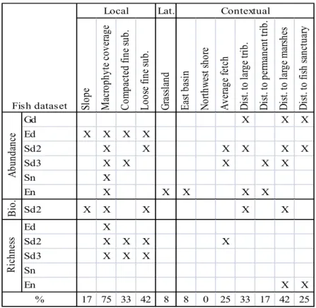
Key variable assessment showed that among local habitat variables, macrophyte coverage, compacted fine substrate and loose fine substrate explained the most variation in FPM having been selected in 75%, 33% and 42% of reduced fish datasets, respectively (Table III). In their respective datasets, macrophyte coverage was positively correlated with FPM, providing an average regression coefficient of 0.61. Compacted fine substrate exhibited negative correlation with FPM, providing an average regression coefficient of -0.81. Loose fine substrate exhibited positive correlation, providing an average regression coefficient of 0.80. Grassland, the remaining lateral variable, was selected in only one fish dataset despite significance in three fish datasets during scale assessment. Meaning, grassland did not explain enough variation to be selected often in key variable assessment, despite explaining a significant amount of variation by itself in variable type assessment. Among contextual habitat variables, distance to large marshes and distance to large tributaries explained the most variation having been selected in 42% and 33% of reduced fish datasets, respectively. In their respective datasets, distance to large marshes was negatively correlated with FPM, providing an average regression coefficient of -0.10. Distance to large tributaries was also negatively correlated, with an average regression coefficient of -0.12.
Table III: Key variable assessment results for the reduced set of fish datasets. “X” denotes statistical and biological significance of a habitat variable explaining variation within a given fish dataset in at least one forward selection. Percent row indicates the percentage of fish datasets for which a variable was selected at least one time.
Lat. Sl op e M ac ro ph yt e co ve ra ge C om pa ct ed fi ne su b. Lo os e fin e su b. G ra ss la nd Ea st b as in N or th w es t s ho re A ve ra ge fe tc h D is t. to la rg e tri b. D is t. to p er m an en t t rib . D is t. to la rg e m ar sh es D is t. to fi sh sa nc tu ar y Gd X X X Ed X X X X Sd2 X X X X X X Sd3 X X X X X Sn X En X X X X X B io . Sd2 X X X X X Ed X Sd2 X X X X Sd3 X X X Sn En X X 17 75 33 42 8 8 0 25 33 17 42 25 % Fish dataset Local Contextual A bu nd an ce R ic hn es s
Discussion
Relative contributions of local, lateral and contextual habitat variables were compared to explain variations in abundance, biomass and richness metrics of fish in the littoral zone of a reservoir. Variable type assessment showed that local and contextual habitat variables contributed similarly to explaining variation across abundance, biomass and richness metrics, whereas lateral habitat variables contributed minimally. While it is clear local habitat variables on average explained more variation across metrics (21% R2adj), the proportion of variation explained by contextual habitat variables (14% R2adj) cannot be overlooked. Similar explanatory power among local and contextual habitat variables suggests both fine- and broad-scale habitat variables explain variation in FPM. This finding is supported by Wang et al. (2003) who found local (reach-scale) variables explained the most inter-river variation in abundance (21% R2), succeeded by contextual (watershed-scale) variables (11% R2); lateral (riparian-scale) variables explained the least variation (5% R2). Bouchard and Boisclair (2008) also observed that local habitat variables explained most variation in intra-river abundance (31% R2adj), succeeded by contextual (longitudinal) variables (1% R2adj); lateral variables failed to explain any variation. In both studies, including local and contextual variables increased explanatory power of models, as opposed to using only local variables to explain variation. Brind'Amour et al. (2005) also observed that fetch (contextual variable) and to a lesser degree macrophytes (local variable) best explained variation in fish community composition in the littoral zone of a Québec lake. The present study reinforces these findings previously made in inter- and intra-river and lake studies, broadening them to intra-reservoir studies. Among studies, similar values of variation explained among several types of habitat variables suggest that the ability to explain variation in FPM in rivers, lakes and reservoirs is similar.
Key variable assessment identified habitat variables most effective at explaining variation across metrics. Macrophyte coverage (local) was selected most often (75%) across metrics as statistically and biologically significant. Compacted fine substrate and loose fine substrate (local) were highly correlated (|r| = 73%) with macrophyte coverage; because these variables were highly correlated and selected less often across metrics, these two variables
may be redundant given macrophyte coverage. Numerous studies have noted macrophytes provide productive feeding environments, refuge from predators, and reproductive environments for phytophilic fish species (Bolding et al. 2004, Dibble et al. 1997, Randall et al. 1996). Effective contextual habitat variables included distance to large marshes (42%) and distance to large tributaries (33%). Marshes have been cited to provide spawning and nursery habitat for a majority of a fish community (Wei et al. 2004), while tributaries may provide complementary resources such as thermal refuge or alternate food sources (Bruns et al. 1984, Dunning et al. 1992). Similar contextual habitat variables were used by Wang et al. (2003), Bouchard and Boisclair (2008) and Brind'Amour et al. (2005) however these similar variables were not among the most important habitat variables explaining variation in abundance. Distance to large marshes and distance to large tributaries had an average negative correlation with FPM. Meaning, abundance, biomass or richness decrease as (site) distance to large marshes or large tributaries increase. Out of all habitat variables, macrophyte coverage explained variation in FPM most effectively; in 75% of reduced fish datasets (Table III) this variable was positively correlated with abundance, biomass or richness, inferring this variable positively influences FPM. Randall et al. (1996) demonstrated macrophyte coverage to be a statistically significant variable (≤ 0.01 p-value) in three different models detailing abundance, biomass and richness of littoral zone fish in the Great Lakes given a series of habitat variables which also included slope (local variable) and fetch. Cvetkovic et al. (2009) also demonstrated that macrophyte coverage was a better predictor of abundance when compared to water quality variables in coastal wetlands of the Georgian Bay (Great Lakes).
Given the results of this study and the findings of others, we have shown the usefulness of using both local and contextual habitat variables to explain variation in FPM of littoral fish communities. Expanding the spatial scope of habitat variables used in fish habitat modeling has allowed us, and others, to capture more variation beyond historically local-based fish habitat models. At the same time, we have shown that lateral habitat variables have little influence on FPM, inferring that littoral fish production is by and large unaffected by terrestrial vegetation type or land use (Table I) that characterizes the shore. In the context of habitat loss or alteration, this finding suggests that maintaining or increasing macrophyte coverage (e.g. Power 1996, Zhao et al. 2012) may contribute to stable or increased littoral fish
productivity. On the other hand, anthropogenic activities that diminish or compromise macrophyte growth may presumably contribute to a decrease in littoral fish productivity.
In this study we have successfully compared relative contributions of local, lateral and contextual habitat variables to explain variation in fish abundance, biomass and richness metrics and identified habitat variables most effective at explaining these variations. In doing so, we have provided a guideline that will allow others to estimate, and ultimately predict littoral FPM based on local and contextual habitat variables present within reservoirs. We presume this study to be applicable to reservoirs and lakes of similar character (i.e. turbid, mesotrophic and windswept); using local and contextual habitat variables, these same methods can be performed to explain variation in littoral FPM. Future studies should focus on an expanded study area beyond a single system to include multiple reservoirs or lakes; this would allow for more generalizable models across systems, and build upon our results and the findings of inter and intra-river and lake studies.
In conclusion, we suggest using a combination of local and contextual habitat variables to explain variation in FPM in the littoral zone of reservoirs. Our results complement the findings of similar studies, allowing us to suggest that productivity is by and large affected by local and contextual habitat variables and less so by lateral variables within the littoral zone of reservoirs, lakes and rivers.
General Conclusion
The findings of this study have implications for researchers, fisheries managers, government, industry and the public. In a broad sense, we have learned that both fine and broad forms of habitat may have an impact on fisheries productivity metrics. Therefore quality habitat at the local level and watershed level is likely an important consideration in maintaining or improving FPM. Specifically, we learned that macrophyte coverage explained variation in FPM most effectively, meaning macrophytes best explained why abundance, biomass or richness were high or low. Furthermore, a positive correlation between macrophyte coverage and abundance, biomass and richness allows us to infer this variable positively influences FPM. These findings give insight into how habitat can be optimally managed to influence FMP, and suggest a more holistic approach to managing fisheries resources.
In the preface, examples demonstrating the need for such research were presented. One example was how to maintain fisheries productivity in light of development, like hydroelectric generation. Another example referred to maintaining or increasing fisheries productivity in response to fish as valuable source of animal protein in developing nations. Given the findings of our study I believe a few suggestions can be made for these examples. In terms of development, we must be concerned not only for site-specific habitat alterations, but also alterations on a spatially larger scale. In addition, our findings may be useful for reservoir planning or improving productivity in existing systems; for example frequent fluctuations in water levels can be planned to submerge macrophytes and encourage new macrophyte growth (e.g. Zhao et al. 2012), likely stimulating fisheries productivity. On a similar note, our findings also suggest that habitat can be manipulated to manage productivity; increasing macrophyte coverage (e.g. Power 1996, Zhao et al. 2012) may contribute to stable or increase littoral fish productivity. Because nearly one billion people rely on fish as their primary source of animal protein, especially in developing nations (WHO/FAO Joint Expert Consultation 2003), I feel compelled to develop fish habitat models to understand what drives productivity there. Similar studies could be initiated with the goal of understanding what
components of habitat most influence fisheries productivity, and be used to better manage and optimize productivity for those who truly depend on it.
The novelty of this study was its execution in a reservoir setting, a system part lotic and lentic in terms of flowing water. Without other reservoir-centric studies to base our study on, we turned to studies of similar scope executed in rivers and lakes to build methodology, make comparisons and draw conclusions. We found similar results suggesting that local and contextual habitat variables best explained variations in abundance, respectively (e.g. Bouchard and Boisclair 2008, Wang et al. 2003) and that macrophyte coverage explained variation in fisheries productivity metrics most effectively (e.g. Cvetkovic et al. 2009, Randall et al. 1996). In closing, we hope our study will serve as guideline allowing others to estimate, and ultimately predict littoral FPM based on local and contextual habitat variables. We have shown the potential of these findings in the context of development and sustainable fisheries, and encourage others to further develop fish habitat models according to their needs.
References
Austin, M. 2002. Spatial prediction of species distribution: an interface between ecological theory and statistical modelling. Ecological modelling 157(2): 101-118. doi: 10.1016/S0304-3800(02)00205-3.
Begon, M., Harper, J.L., and Townsend, C.R. 1990. Ecology: Individuals, Populations, and Communities. Blackwell Scientific Publications, Boston, M.A.
Bolding, B., Bonar, S., and Divens, M. 2004. Use of Artificial Structure to Enhance Angler Benefits in Lakes, Ponds, and Reservoirs: A Literature Review. Reviews in Fisheries Science
12(1): 75-96. doi: 10.1080/10641260490273050.
Borcard, D., Legendre, P., and Drapeau, P. 1992. Partialling out the spatial component of ecological variation. Ecology 73(3): 1045-1055. doi: 10.2307/1940179
Bouchard, J., and Boisclair, D. 2008. The relative importance of local, lateral, and longitudinal variables on the development of habitat quality models for a river. Canadian Journal of
Fisheries and Aquatic Sciences 65(1): 61-73. doi: 10.1139/f07-140
Brind'Amour, A., and Boisclair, D. 2004. Comparison between two sampling methods to evaluate the structure of fish communities in the littoral zone of a Laurentian lake. Journal of Fish Biology 65(5): 1372-1384. doi: 10.1111/j.0022-1112.2004.00536.x.
Brind'Amour, A., Boisclair, D., Legendre, P., and Borcard, D. 2005. Multiscale spatial
distribution of a littoral fish community in relation to environmental variables. Limnology and Oceanography 50(2): 465-479. doi: 10.4319/lo.2005.50.2.0465.
Bruns, D., Minshall, G., Cushing, C., Cummins, K., Brock, J., and Vannote, R. 1984. Tributaries as modifiers of the river continuum concept: analysis by polar ordination and regression models. Archiv für Hydrobiologie 99(2): 208-220.
Bryan, M.D., and Scarnecchia, D.L. 1992. Species richness, composition, and abundance of fish larvae and juveniles inhabiting natural and developed shorelines of a glacial Iowa lake. Environmental Biology of Fishes 35(4): 329-341. doi: 10.1007/BF00004984.
Crowder, L.B., and Cooper, W.E. 1982. Habitat Structural Complexity and the Interaction Between Bluegills and Their Prey. Ecology 63(6): 1802-1813. doi: 10.2307/1940122. Cvetkovic, M., Wei, A., and Chow-Fraser, P. 2009. Relative importance of macrophyte community versus water quality variables for predicting fish assemblages in coastal wetlands of the Laurentian Great Lakes. Journal of Great Lakes Research 36(1): 64-73. doi:
10.1016/j.jglr.2009.10.003.
Denton, J.A. 1990. Society and the Official World: A Reintroduction to Sociology. Rowman & Littlefield, Lanham, M.D.
Dibble, E.D., Killgore, K.J., and Harrel, S.L. 1997. Assessment of fish-plant interactions A-97-6. U.S. Army Corps of Engineers, Vicksburg, M.S.
Dray, S., Legendre, P., and Blanchet, G. 2011. packfor: Forward Selection with permutation (Canoco p.46). R package version 0.0-8/r100. Available from
http://R-Forge.R-project.org/projects/sedar.
Duarte, C.M., and Kalff, J. 1986. Littoral slope as a predictor of the maximum biomass of submerged macrophyte communities. Limnology and Oceanography 31(5): 1072-1080. doi: 10.4319/lo.1986.31.5.1072.
Dunning, J.B., Danielson, B.J., and Pulliam, H.R. 1992. Ecological processes that affect populations in complex landscapes. Oikos 65(1): 169-175. doi: 10.2307/3544901 Environment Canada. 2013. Pinawa, Manitoba. Available from
http://climate.weather.gc.ca/climateData/dailydata_e.html?StationID=10186 [accessed May 9 2013].
ESRI. 2013. ArcGIS Desktop 10.2. Redlands, California.
Evans, D.O., Nicholls, K.H., Allen, Y.C., and McMurtry, M.J. 1996. Historical land use, phosphorus loading, and loss of fish habitat in Lake Simcoe, Canada. Canadian Journal of Fisheries and Aquatic Sciences 53(S1): 194-218. doi: 10.1139/f96-012.
Fortin, M.-J., Dale, M.R., and Ver Hoef, J.M. 2002. Spatial analysis in ecology. In Encyclopedia of Environmetrics. Edited by A.H. El-Shaarawi and W.W. Piegorsch. John Wiley & Sons, Ltd, Chichester, England. pp. 2051–2058.
Gamboa-Pérez, H., and Schmitter-Soto, J. 1999. Distribution of cichlid fishes in the littoral of Lake Bacalar, Yucatan Peninsula. Environmental Biology of Fishes 54(1): 35-43. doi:
10.1023/A:1007443408776.
Google Earth 7.1. 2007. Lat. 50.360548°, Lon. -95.897501°, elev. 812. Available from http://www.google.com/earth/index.html [accessed October 2013].
Guegan, J.-F., Lek, S., and Oberdorff, T. 1998. Energy availability and habitat heterogeneity predict global riverine fish diversity. Nature 391(6665): 382-384. doi: 10.1038/34899. Guisan, A., and Zimmermann, N.E. 2000. Predictive habitat distribution models in ecology. Ecological Modelling 135(2–3): 147-186. doi: 10.1016/S0304-3800(00)00354-9.
Harris, J., and Silveira, R. 1999. Large-scale assessments of river health using an Index of Biotic Integrity with low-diversity fish communities. Freshwater Biology 41(2): 235-252. doi: 10.1046/j.1365-2427.1999.00428.x.
Hoekstra, J.M., Boucher, T.M., Ricketts, T.H., and Roberts, C. 2005. Confronting a biome crisis: global disparities of habitat loss and protection. Ecology Letters 8(1): 23-29. doi: 10.1111/j.1461-0248.2004.00686.x.
Inoue, M., and Nakano, S. 2001. Fish abundance and habitat relationships in forest and grassland streams, northern Hokkaido, Japan. Ecological Research 16(2): 233-247. doi: 10.1046/j.1440-1703.2001.00389.x.
Kruse, C.G., Hubert, W.A., and Rahel, F.J. 1997. Geomorphic Influences on the Distribution of Yellowstone Cutthroat Trout in the Absaroka Mountains, Wyoming. Transactions of the American Fisheries Society 126(3): 418-427. doi:
Minns, C.K. 1997. Quantifying “no net loss” of productivity of fish habitats. Canadian Journal of Fisheries and Aquatic Sciences 54(10): 2463-2473. doi: 10.1139/f97-149.
Morrison, M.L., Marcot, B., and Mannan, W. 2012. Wildlife-Habitat Relationships: Concepts and Applications. Island Press, Washington, D.C.
Murphy, B.R., and Willis, D.W. 1996. Fisheries Techniques. American Fisheries Society, Bethesda, M.D.
Nelson, R.L., Platts, W.S., Larsen, D.P., and Jensen, S.E. 1992. Trout Distribution and Habitat in Relation to Geology and Geomorphology in the North Fork Humboldt River Drainage, Northeastern Nevada. Transactions of the American Fisheries Society 121(4): 405-426. doi: 10.1577/1548-8659(1992)121<0405:TDAHIR>2.3.CO;2.
Odum, E.P. 1971. Fundamentals of Ecology. W.B Sounders, Philadelphia, P.A.
Oksanen, J., Blanchet, F.G., Kindt, R., Legendre, P., Minchin, P.R., O'Hara, R.B., Simpson, G.L., Solymos, P., Stevens, M.H.H., and Wagner, H. 2012. vegan: Community Ecology Package. R package version 2.0-5. Available from http://CRAN.R-project.org/package=vegan. Olden, J.D., and Jackson, D.A. 2001. Fish–Habitat Relationships in Lakes: Gaining Predictive and Explanatory Insight by Using Artificial Neural Networks. Transactions of the American Fisheries Society 130(5): 878-897. doi:
10.1577/1548-8659(2001)130<0878:FHRILG>2.0.CO;2.
Pegg, M.A., and Pierce, C.L. 2002. Fish community structure in the Missouri and lower Yellowstone rivers in relation to flow characteristics. Hydrobiologia 479(1-3): 155-167. doi: 10.1023/A:1021038207741.
Pierce, C.L., Rasmussen, J.B., and Leggett, W.C. 1990. Sampling littoral fish with a seine: corrections for variable capture efficiency. Canadian Journal of Fisheries and Aquatic Sciences 47(5): 1004-1010. doi: 10.1139/f03-098.
Porter, M.S., Rosenfeld, J., and Parkinson, E.A. 2000. Predictive Models of Fish Species Distribution in the Blackwater Drainage, British Columbia. North American Journal of Fisheries Management 20(2): 349-359. doi:
10.1577/1548-8675(2000)020<0349:PMOFSD>2.3.CO;2.
Power, P.J. 1996. Reintroduction of Texas wildrice (Zizania texana) in Spring Lake: some important environmental and biotic considerations. United States Department of Agriculture Forest Service General Technical Report RM-GTR-283 0277-5786.
Pratt, T.C., and Smokorowski, K.E. 2003. Fish habitat management implications of the
summer habitat use by littoral fishes in a north temperate, mesotrophic lake. Canadian Journal of Fisheries and Aquatic Sciences 60(3): 286-300. doi: 10.1139/f03-022.
Quiros, R. 1990. Predictors of Relative Fish Biomass in Lakes and Reservoirs of Argentina. Canadian Journal of Fisheries and Aquatic Sciences 47(5): 928-939. doi: 10.1139/f90-107. R Core Team. 2012. R: A language and environment for statistical computing. R Foundation for Statistical Computing, Vienna, Austria. ISBN 3-900051-07-0. Available from
Rahel, F.J. 1984. Factors Structuring Fish Assemblages Along a Bog Lake Successional Gradient. Ecology 65(4): 1276-1289. doi: 10.2307/1938333.
Randall, R.G., Minns, C.K., and Brousseau, C.M. 2004. Coastal exposure as a first-order predictor of the productive capacity of near shore habitat in the Great Lakes 2004/087. Fisheries and Oceans Canada, Burlington, O.N.
Randall, R.G., Minns, C.K., Cairns, V.W., and Moore, J.E. 1996. The relationship between an index of fish production and submerged macrophytes and other habitat features at three littoral areas in the Great Lakes. Canadian Journal of Fisheries and Aquatic Sciences 53: 35-44. doi: 10.1139/f95-271.
Randall, R.G., Minns, C.K., Cairns, V.W., Moore, J.E., and Valere, B. 1998. Habitat
predictors of fish species occurrence and abundance in nearshore areas of Severn Sound 2440. Fisheries and Oceans Canada, Burlington, O.N.
Reyjol, Y., Rodríguez, M.A., Dubuc, N., Magnan, P., and Fortin, R. 2008. Among- and
within-tributary responses of riverine fish assemblages to habitat features. Canadian Journal of Fisheries and Aquatic Sciences 65(7): 1379-1393. doi: 10.1139/F08-060.
Richter, B.D., Braun, D.P., Mendelson, M.A., and Master, L.L. 1997. Threats to Imperiled Freshwater Fauna. Conservation Biology 11(5): 1081-1093. doi:
10.1046/j.1523-1739.1997.96236.x.
Rieman, B.E., and McIntyre, J.D. 1995. Occurrence of Bull Trout in Naturally Fragmented Habitat Patches of Varied Size. Transactions of the American Fisheries Society 124(3): 285-296. doi: 10.1577/1548-8659(1995)124<0285:OOBTIN>2.3.CO;2.
Savino, J.F., and Stein, R.A. 1982. Predator-Prey Interaction between Largemouth Bass and Bluegills as Influenced by Simulated, Submersed Vegetation. Transactions of the American Fisheries Society 111(3): 255-266. doi:
10.1577/1548-8659(1982)111<255:PIBLBA>2.0.CO;2.
Senay, C., Boisclair, D., and Peres-Neto, P.R. 2014. Habitat-based polymorphism is common in stream fishes. Journal of Animal Ecology 84(1): 219-227. doi: 10.1111/1365-2656.12269. Southwood, T.R.E. 1977. Habitat, the Templet for Ecological Strategies? Journal of Animal Ecology 46(2): 337-365. doi: 10.2307/3817.
Stang, D., and Hubert, W. 1984. Spatial separation of fishes captured in passive gear in a turbid prairie lake. Environmental Biology of Fishes 11(4): 309-314. doi:
10.1007/BF00001378.
Trombulak, S.C., and Frissell, C.A. 2000. Review of Ecological Effects of Roads on Terrestrial and Aquatic Communities. Conservation Biology 14(1): 18-30. doi: 10.1046/j.1523-1739.2000.99084.x.
Wall, S.S., Berry, J.C.R., Blausey, C.M., Jenks, J.A., and Kopplin, C.J. 2004. Fish-habitat modeling for gap analysis to conserve the endangered Topeka shiner (Notropis topeka). Canadian Journal of Fisheries and Aquatic Sciences 61(6): 954-973. doi: 10.1139/f04-017.