CIRPÉE
Centre interuniversitaire sur le risque, les politiques économiques et l’emploi
Cahier de recherche/Working Paper 06-41
Decomposition of s ― Concentration Curves
Paul Makdissi Stéphane Mussard
Novembre/November 2006
_______________________
Makdissi: CIRPÉE and GRÉDI, Département d’économique, Université de Sherbrooke, 2500, boulevard de l’Université, Sherbrooke, Québec, Canada J1K 2R1
Mussard: Corresponding author. CEPS/INSTEAD Luxembourg, GRÉDI Université de Sherbrooke and GEREM Université de Perpignan. Address: Département des Sciences Économiques, Université de Perpignan, 52 avenue Paul Alduy, 66860 Perpignan Cedex, France
This paper was partly done when Stéphane Mussard was post-doctoral researcher at CEPS / INSTEAD Luxembourg and when he visited the University of Sherbrooke and GRÉDI, which are greatly acknowledged. He is also greatly indebted to the Ministère de la Recherche du Luxembourg and GRÉDI for financial support.
Abstract:
For any given order of stochastic dominance, standard concentration curves are decomposed into contribution curves corresponding to within-group inequalities, between-group inequalities, and transvariational inequalities. We prove, for all orders, that contribution curve dominance implies systematically welfare-improving tax reforms and conversely. Accordingly, we point out some undesirable fiscal reforms since a welfare expansion may be costly in terms of particular inequalities.
Keywords: Concentration curves, Contribution curves, Stochastic dominance, Tax
reforms
1 Introduction
Yitzhaki and Slemrod (1991) and subsequently Yitzhaki and Thirsk (1990) demonstrated that tax reforms, for pairs of commodities or multiple com-modities, can be welfare improving with non-intersecting concentration curves for all additively separable social welfare functions and all increasing S-concave social welfare functions. In 1991, they applied their technique on the extended Gini coefficient. Accordingly, if the concentration curve of good i dominates (lies above) that of good j, in other words, if there are less inequalities in good i than in good j, then an increasing tax on good j com-bined with a decreasing tax on good i enables decision makers to improve overall welfare or equivalently to decline overall inequalities.
When the population is partitioned in many groups, a usual way to analyze the structure of income inequalities, referring to the Gini index, is to decompose the overall inequality (see e.g. Lerman and Yitzhaki (1991), Dagum (1997a, 1997b) or Aaberge et al. (2005) among others) in a within-group index GW, an average between-group index GB, and a transvariational
index GT.1 The latter, being different from a residual, gauges between-group
inequalities issued from the groups with lower mean incomes.
In this note, we aim at using the subgroup decomposition technique of the Gini index initiated by Lambert and Aronson (1993) in order to show that standard welfare-improving tax reforms, for pairs of commodities
{i, j}, can be performed with less within-group inequalities, less
between-group inequalities in mean, and more transvariational inequalities in good
i than in good j. In other words, instead of looking for non-intersecting
concentration curves, we provide stronger conditions allowing for welfare-improving tax reforms on goods {i, j} by introducing contribution curves for all determinants of overall inequality, namely: within-group, between-group, and transvariational contribution curves. Contrary to the results related to traditional concentration curves (see e.g. Makdissi and Mussard (2006)), we show that, for any order, it is sufficient but not necessary that all contribution curves of good j lie above those of good i, except for the transvariational contribution curve.
The note is attacked as follows. Section 2 reviews Lambert and Aronson’s (1993) Gini decomposition. Section 3 introduces notations and definitions. Section 4 explores welfare-improving tax reforms with the concept of
contri-1See also the Gini decompositions of Bhattacharya and Mahalanobis (1967), Rao
(1969), Pyatt (1976), Silber (1989), Lambert and Aronson (1993), Sastry and Kelkar (1994), Deutsch and Silber (1999).
bution curves for all order of stochastic dominance. Section 5 is devoted to the concluding remarks.
2 Subgroup Decomposition of the Lorenz Curve
In this section, we briefly summarize the results obtained by Lambert and Aronson (1993). Let a population Π of size n and mean income µ be parti-tioned into K groups: Π1, . . . , Πk, . . . , ΠK of size nk and mean income µk.
The groups are ranked as follows: µ1 ≤ . . . ≤ µk ≤ . . . ≤ µK. Assume the individuals are ranked within each Πk such as the richest person of Πk−1
is just positioned before the poorest one of Πk. Then, the rank of an
in-dividual belonging to Πk is given by: p(pk) =
Pk−1
i=1ni+pknk
n . Therefore, the
within-group Lorenz curve LW(p(pk)) is formalized to compute inequalities
within groups:
LW(p(pk)) =
Pk−1
i=1 niµi+ nkµkLk(pk)
nµ , (1)
where Lk(pk) is the Lorenz curve associated with group Πk.2 The Lorenz
curve between groups, LB(p), is obtained by considering that each individual
within Πk earns the mean income of his group µk such as the total income
PK
k=1nkµk is redistributed among the groups:
LB(p(pk)) =
Pk−1
i=1 niµi+ nkµkpk
nµ . (2)
The use of these different Lorenz curves yields the overall breakdown of the Gini index (G) in three components: G = GW+ GB+ GT. The contribution
of the inequalities within groups (or the within-group Gini) is:
GW = 2
Z 1 0
[LB(p) − LW(p)] dp. (3)
The contribution of the inequalities between groups in mean (or the between-group Gini) is:
GB = 2
Z 1 0
[p − LB(p)] dp. (4)
2To avoid confusions with further notations, we use L
W(pk). In the traditional version of Lambert and Aronson’s (1993) article, LW(·) is denoted C(·) with respect to the tra-ditional concentration curve. Indeed, as individuals are ranked by incomes (in ascending order within each group), C(p) measures the proportion of total income received by the first np individuals.
The contribution of the transvariation between groups (or the Gini of transvari-ation) is: GT = 2 Z 1 0 [LW(p) − L(p)] dp, (5)
where L(p) is the Lorenz curve associated with the global population.3 The transvariation (see Gini (1916), Dagum (1959, 1960, 1961), Deutsch and Silber (1997), among others) brings out the intensity with which the groups are polarized. The greater the transvariation is, or equivalently, the wider the overlap between the distributions is, the lower the polarization may be.
3 Notations and Definitions
The Lorenz curve constitutes the basis of the preceding reasoning of de-composition. As a consequence, for any given consumption good (say j), we gauge the proportion of total consumption of j received by the first np individuals ranked by ascending order of consumption. In the sequel, we use an analogous scheme of decomposition. However, it is related to concentra-tion curves C2(p), C2
j(p) being that of good j. We analyze the proportion
of total consumption of j received by the first np individuals ranked by as-cending order of income. In order to decompose concentration curves, we take recourse to the same lexicographic parade introduced by Lambert and Aronson (1993).
Definition 3.1 Let pk be the rank of a person in Πk according to her income
such as p(pk) =
Pk−1
i=1ni+pknk
n , and µ
j
k the k-th group’s average consumption of
good j such as: µj1 ≤ . . . ≤ µjk≤ . . . ≤ µjK. The between-group concentration curve and the within-group concentration curve of the j-th commodity are expressed as, respectively:
CjB2 (p(pk)) = Pk−1 i=1 niµ j i + nkµjkpk nµj (6) C2 jW(p(pk)) = Pk−1 i=1 niµji + nkµjkCjk2 (pk) nµj , (7) with C2
jk(pk) being the concentration curve of group Πk for good j.
3Note that this technique of decomposition is different from those of Dagum (1997a,
1997b), where the inequalities between groups (in mean or transvariation) involve variance and asymmetrical effects between groups, and where GT is non negative (see also Berrebi and Silber (1987) to learn more about the Gini index with dispersion and asymmetry). Here, LW(p) − L(p) can be negative, then GT can also be negative (see also Lerman and Yitzhaki (1991)).
The decomposition technique exhibits different concentration amounts prevailing in a given population. These are related to the number of indi-viduals within each group. Then, one obtains contribution indices, namely, within-group, between-group and transvariational contributions to the over-all concentration measure. Indeed, these ”population-based measures” ex-plicitly involve the population shares of each Πk group (see e.g. Rao (1969)).
Consequently, these contribution indicators may then be helpful to address issues in the design of indirect tax reforms. For this purpose, we formalize theses contribution indices by initiating the concept of contribution curves. Note that a similar notion, used by Duclos and Makdissi (2005), enables contribution curves of poverty measures to be conceived.4
Definition 3.2 The within-group contribution curve (CCjW), the
between-group contribution curve (CCjB), and the transvariational contribution curve
(CCjT) of the j-th commodity yield a linear breakdown of the concentration
curve of good j: CCjW(p) : = CjB2 (p) − CjW2 (p) CCjB(p) : = p − CjB2 (p) CCjT(p) : = CjW2 (p) − Cj2(p) =⇒ C2 j(p) = p − CCjW(p) − CCjB(p) − CCjT(p). (8)
The contribution curves coincide with second-degree stochastic dominance.5 Remark that, integrating any given contribution curve provides a precise contribution to the overall concentration index (C). For instance, CW :=
2R01[CCjW(p)] dp yields the absolute contribution of the within-group
con-centration to the global amount of concon-centration in good j. In the same man-ner, one obtains the absolute contribution of between-group and transvari-ational concentrations, respectively, CB := 2
R1
0 [CCjB(p)] dp and CT := 2R01[CCjT(p)] dp, such as: C = CW + CB+ CT.
For the need of Section 4, s-order concentration curves are introduced. Definition 3.3 (Makdissi and Mussard (2006)). The first-order
concentra-tion curve defined as C1
m(p) = xm(p) /Xm, is the consumption of good m
for an individual at rank p divided by the average consumption of the good. The s-concentration curve is then given by: Cs
m(p) =
Rp
0 Cms−1(u) du.
4The fact that many persons are affected by poverty or by inequality motivates the
use of contribution curve concepts for dominance purposes.
5Alternatively, one may consider, as in Aaberge (2004), that first-order dominance is
Lorenz dominance. Here, s-order dominance is related to s-concentration curves intro-duced in Definition 3.3.
4 Fiscal Reform Impacts
Let us define the environment on which we intend to obtain welfare-improving tax reforms. On the one hand, we consider the following rank dependant social welfare function (see Yaari (1987, 1988)):
W (F ) =
Z 1 0
F−1(p) v (p) dp (H1)
where F−1(p) = inf©yE : F¡yE¢ ≥ pª is the left continuous inverse income
distribution, yE the equivalent income, F ¡yE¢ the distribution of
equiva-lent income, and v (p) ≥ 0 the frequency distortion function weighting an individual at the p-th percentile of the distribution. On the other hand, we impose this distortion function being continuous and s-time differentiable almost everywhere over [0, 1]:
(−1)`v(`)(p) ≥ 0 , ` ∈ {1, 2, . . . , s}, (H2) where v(`)(·) is the `-th derivative of the v (·) function, v(0)(·) being the function itself. Finally, we restrict our study on the following class of social welfare functions:
e
Ωs :=©W (·) ∈ {H1 ∩ H2} : (−1)`v(`)(1) = 0, ` ∈ {1, 2, . . . , s}ª. (H3) Suppose the government plans a decreasing tax on good i with an increas-ing tax on good j, lettincreas-ing his budget constant. This marginal tax reform entails a variation in equivalent income F−1(p) for an individual at rank p:
dF−1(p) = ∂F−1(p) ∂ti dti+ ∂F−1(p) ∂tj dtj. (9)
As shown by Besley and Kanbur (1988), the change in the equivalent income induced by a marginal change in the tax rate of good i is:
∂F−1(p)
∂ti
= −xi(p) , (10)
where xi(p) is the Marshallian demand of good i of the individual at rank p in
the income distribution. Let M be the number of goods, m ∈ {1, 2, . . . , M }. Suppose a constant average tax revenue, dR = 0, where R = PMm=1tmXm
and where Xm is the average consumption of the m-th commodity: Xm =
R1
0 xm(p) dp. Yitzhaki and Slemrod (1991) prove that constant producer prices induce: dtj = −α µ Xi Xj ¶ dti where α = 1 + 1 Xi PM m=1tm∂X∂tmi 1 + 1 Xj PM m=1tm∂X∂tjm . (11)
Wildasin (1984) interprets α as the differential efficiency cost of raising one dollar of public funds by taxing the j-th commodity and using the proceeds to subsidize the i-th commodity. Substituting (11) and (10) in (9) yields:
dF−1(p) = − · xi(p) Xi − αxj(p) Xj ¸ Xidti. (12)
Following Definition 3.1, equation (12) can be rewritten as:
dF−1(p) = −£Ci1(p) − αCj1(p)¤Xidti. (13)
Consequently, following H1, the variation of social welfare induced by an indirect tax reform is:
dW (F ) = −Xidti Z 1 0 £ C1 i (p) − αCj1(p) ¤ v (p) dp. (14)
Theorem 4.1 A revenue-neutral marginal tax reform, dtj = −α
³
Xi
Xj
´
dti >
0 with α ≤ 1, implies dW (·) ≥ 0 for all W (·) ∈ eΩs, for any given s ∈
{2, 3, 4, . . .}, if and only if αCCs−1 jW (p) − CCiWs−1(p) + αCCs−1 jB (p) − CCiBs−1(p) (15) + αCCjTs−1(p) − CCiTs−1(p) ≥ 0, for all p ∈ [0, 1] . Proof. See the Appendix.
Note that the specification of within-group contribution curves brings out the average within-group inequalities. It turns out that, it would be appeal-ing to formalize a taxation technique ensurappeal-ing decision makers that welfare-improving tax reforms reduce inequalities within all subgroups. Indeed, this condition is not guaranteed in Theorem 4.1, for which within-group inequal-ities in mean may only be reduced for good j (if αCCjWs−1 dominates CCiWs−1 for α ≤ 1). Subsequently, if we were able to construct within-group contri-bution curves for all groups Πk, k ∈ {1, 2, . . . , K}, (say CCjW,ks−1 for the j-th
commodity) and to find a couple of goods {i, j} that guarantees dominance between within-group contribution curves for all Πk, then we could find a
welfare-improving tax reform that decreases inequalities within each group. This outcome culminates in the following theorem.
Theorem 4.2 A revenue-neutral marginal tax reform, dtj = −α ³ Xi Xj ´ dti >
0 with α ≤ 1, implies dW (·) ≥ 0 for all W (·) ∈ eΩs, for any given s ∈
{2, 3, 4, . . .}, if and only if K X k=1 £ αCCs−1 jW,k(p) − CCiW,ks−1(p) ¤ + αCCs−1 jB (p) − CCiBs−1(p) (16) + αCCs−1 jT (p) − CCiTs−1(p) ≥ 0, for all p ∈ [0, 1] .
Proof. See the Appendix.
Following Theorem 4.2, a wide range of tax programs are operational with different constraints.
Proposition 4.3 Three particular solutions of Eq. (16) are:
S1 := © αCCjW,ks−1 (p) ≥ CCiW,ks−1(p) ∀k ∈ {1, 2, . . . , K}, s ∈ {2, 3, 4, . . .} : K X k=1 £ αCCjW,ks−1(p) − CCiW,ks−1(p)¤ ≥ CCs−1 jB (p) − CCiBs−1(p) + αCCjTs−1(p) − CCiTs−1(p) ª , S2 := © αCCs−1 jB (p) ≥ CCiBs−1(p), s ∈ {2, 3, 4, . . .} : αCCs−1 jB (p) − CCiBs−1(p) ≥ K X k=1 £ αCCs−1 jW,k(p) − CCiW,ks−1(p) ¤ + αCCs−1 jT (p) − CCiTs−1(p) ≥ 0 ) , S3 := © αCCs−1 jT (p) ≤ CCiTs−1(p), s ∈ {2, 3, 4, . . .} : K X k=1 £ αCCs−1 jW,k(p) − CCiW,ks−1(p) ¤ + αCCs−1 jB (p) − CCiBs−1(p) ≥ CCiTs−1(p) − αCCjTs−1(p)ª. Proof. It is straightforward.
(S1) This first solution postulates that all within-group contribution curves of good j dominate those of good i, provided the former is multiplied by α. The condition is that the dominance sum is sufficiently important compared with the remaining terms. Then, an increasing tax on good j, for which the repartition is favorable to rich people, coupled with a decreas-ing tax on good i produces systematically an overall welfare improvement
with alleviation of inequalities within each group, for any s-order stochastic dominance.6
(S2) If the between-group contribution curve of the j-th commodity (mul-tiplied by α) lies above that of the i-th commodity, provided Eq. (16) re-mains positive, then an increasing tax on the j-th commodity coupled with a decreasing tax on the i-th commodity yields necessarily an increase of wel-fare with a between-group inequality reduction, for any s-order stochastic dominance.
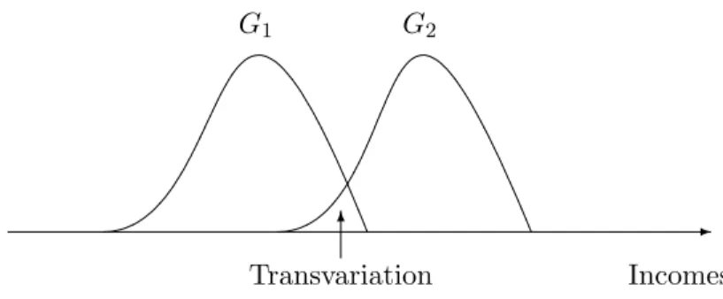
(S3) The third case is an atypical one. Indeed, welfare-improving tax reforms might be performed with a reduction in transvariational inequalities. Nevertheless, as depicted in Figure 1, it is not a desirable issue.
Figure 1. Inequalities of Transvariation
-Incomes 6
Transvariation
G1 G2
Following Figure 1, when two distributions overlap, inequalities of trans-variation are recorded. This particular concept, inspired from Gini (1916) and subsequently developed by Dagum (1959, 1960, 1961), characterizes the income differences between the group of lower mean income (G1) and that of higher mean income (G2). Transvariation means that between-group differences in incomes are of opposite sign compared with the difference in the income average of their corresponding group. It is closely connected with economic distances (see e.g. Dagum (1980)), stratification indices (see e.g. Lerman and Yitzhaki (1991)) or polarization measures (see e.g. Duclos, Esteban and Ray (2004)). Therefore, S3 suggests that welfare-improving tax reforms can be achieved with a growing transvariation (reduction of polarization) between the groups.
6Other constraints are available for S
1. For instance, αCCjBs−1(p) − CCiBs−1(p) + αCCjTs−1(p) − CCiTs−1(p) ≥ 0, may be viewed as a stronger variant. This remark also holds for S2.
Finally, decision makers can contemplate doing welfare-improving tax reforms subject to the reduction of within-group inequalities, subject to the decline of between-group inequalities or subject to the expansion of transvariational inequalities. However, stronger welfaincreasing tax re-forms may be performed in a combinatoric way: αCCs−1
jW dominates CCiWs−1,
αCCs−1
jB dominates CCiBs−1, and CCiTs−1 dominates αCCjTs−1.7 This
necessar-ily implies a welfare gain with alleviation of within-group and between-group inequalities and with transvariational expansion. The reverse being not true. Application 4.4 A revenue-neutral marginal tax reform, dtj = −α
³
Xi
Xj
´
dti >
0 with α ≤ 1, that increases Gini social welfare functions under the
domi-nance conditions defined in S1, S2, and S3, enables decision makers to choose
between a wide range of inequality aversion parameters ν.
Proof. The class of functions WSG(·), for which v(p) = ν(1 − p)ν−1, is
the well-known family of Gini social welfare functions such as WSG(·) ∈ eΩs.
They are concave if 1 < ν < 2, convex if ν > 2 and consequently yield exactly the same results as in Theorem 4.2, for any given parameter of inequality aversion.
5 Concluding Remarks
The employ of rank dependent social welfare functions is well-suited for the respect of ethical properties such as Pigou-Dalton transfers (Pigou (1912)), a set {Ak} of taxation schemes (Gajdos (2002)), uniform α-spreads (Gajdos (2004)), or the principle of positionalist transfers (see e.g. Zoli (1999) and Aaberge (2004)). For the latter, for all W (·) ∈ eΩs, an income transfer from a
higher-income individual to a lower-income one (say a progressive transfer) yields a better impact on social welfare as far as individuals’ ranks are the lowest as possible. For instance, when s = 2, a progressive transfer occurs. For s = 3, one gets composite transfers, that is, a progressive transfer aris-ing at the bottom of the distribution combined with a reverse progressive transfer at the top. Higher-order principles can be illustrated with Fishburn and Willig’s (1984) general transfer principle, for which composite transfers
7The condition α ≤ 1 yields the set of relevant indirect taxation schemes, see Yitzhaki
and Slemrod (1991, p. 483-485). For instance, the case for which α = 1 is very useful for applications and implies neither efficiency gain nor efficiency loss for the government, but the indirect taxation program remains relevant, see Makdissi and Wodon (2002, p. 230-231.).
occur both at the bottom and at the top of the distribution. Accordingly, one should analyze, not independently, indirect tax reforms and the impli-cation of the dominance ethical properties resulting from the social welfare function. Therefore, if the s-concentration curve of good i dominates that of good j, then s-order dominance and welfare-improving tax reforms may be interpreted as direct tax programs favorable to lower-income persons coupled with indirect tax programs, such as an increasing tax on the j-th commodity (also favorable to lower-income earners) with a decreasing tax on the i-th commodity, implying an overall welfare expansion.
In a more general fashion, we point out undesirable welfare-improving tax reforms, especially when s-concentration curves are not decomposed. Indeed, as the welfare amplification possesses three inequality counterparts characterized by the contribution curves, it turns out that a fiscal reform may be costly in terms of particular consumption inequalities. Accordingly, it seems reasonable to perform welfare-increasing tax reforms in being aware of the underlying inequality entailments: variation of the inequalities within each group, variation of the inequalities between groups and variation of the transvariational inequalities.
Finally, the methodology allows one to deal with Gini social welfare functions that depend on an inequality aversion parameter. This might contribute to shed more light on the possibility for the social planner to adjust the power of the tax reform in function of the inequality aversion.
Appendix
Proof of Theorem 4.1.
(Sufficiency) Integrating successively equation (13) by parts yields:
dW (F ) = −Xidti(−1)s−1 Z 1 0 £ Cs i (p) − αCjs(p) ¤ v(s−1)(p) dp. (A1) Given that −Xidti and (−1)s−1v(s−1) are non negative, it is then sufficient
to have Cs
i (p) − αCjs(p) ≥ 0, ∀p ∈ [0, 1] with s ∈ {1, 2, . . .} in order to
obtain dW (·) ≥ 0. Now, we have to decompose the s-order concentration curves Cs into contribution curves CCl for all l ∈ {1, 2, . . . s − 1}, and to
use a similar dominance reasoning. Order l = 1:
From equation (A1), an increase of overall welfare is given by C2
i (p) −
αC2
good i. Indeed, remark that for any given consumption variable x, ranked by ascending order of income, R01x(p)dp is an approximation of the
arith-metic mean µ. Using the formulae of the sum of trapeze areas, we have: R1 0 x(p)dp = x1p1 2 + (x1+x2)(p2−p1) 2 + . . . + (1−pn−1)(xn−1+xn)
2 . Individual data en-tail pi = nni = n1. Then, R1 0 x(p)dp = x1.1/n 2 + x1.1/n+x2.1/n 2 +. . .+ 1/n.xn−1+1/n.xn 2 = x1+x2+...+xn/2
n ∼= µ. Consequently, the proportion of x detained by the
first np individuals is: P (p) ∼= x1.1/n+x2.1/n+...+xn−1.1/n
µ ∼=
Pn−1 i nixi
nµ , where
p = n−1
n , and where P (0) = 0 and P (1) = 1. From Definition 3.1, it is easy
to see that P (p) = C2(p) ∼= 1/µRp
0 x(u)du. Now remember equation (8):
C2(p) = p − CC
W(p) − CCB(p) − CCT(p) and suppose that these
contribu-tion curves are first-order curves, that is, C2(p) = p − CC1
W(p) − CCB1(p) −
CC1
T(p). In order to get dW ≥ 0 it is sufficient to have Ci2(p) ≥ αCj2(p),
where C2
i(p) and Cj2(p) are respectively concentration curves of goods i and
j. Consequently, in order to to have dW ≥ 0, it is sufficient to match the
following condition for all α ≤ 1:
αCC1 jW (p) − CCiW1 (p) + αCCjB1 (p) − CCiB1 (p) (A2) + αCC1 jT (p) − CCiT1 (p) ≥ 0, for all p ∈ [0, 1] , where CC1
jW is the first-order within-group contribution curve of good j,
CC1
iW the first-order within-group contribution curve of good i, and so on.
Order l − 1:
Now assume we have:
αCCl−1 jW (p) − CCiWl−1(p) + αCCl−1 jB (p) − CCiBl−1(p) (A3) + αCCl−1 jT (p) − CCiTl−1(p) ≥ 0, for all p ∈ [0, 1] .
integrate l − 1 times first-order contribution curves: Cl+1(p) = Z p 0 Z u 0 . . . Z z 0 | {z } l−1 times C2(t)dt . . . du = Z p 0 Z u 0 . . . Z z 0 | {z } l−1 times £ t − CC1 W(t) − CCB1(t) − CCT1(t) ¤ dt . . . du = Z p 0 Z u 0 . . . Z z 0 | {z } l−1 times tdt . . . du − CCl−1 W (p) − CCBl−1(p) − CCTl−1(p). (A4) Order l:
Integrating (A4) for goods i and j leads to:
Cl+2 i (p) = Z p 0 Z u 0 . . . Z z 0 | {z } l times tdt . . . du − CCl iW(p) − CCiBl (p) − CCiTl (p) Cl+2 j (p) = Z p 0 Z u 0 . . . Z z 0 | {z } l times tdt . . . du − CCl jW(p) − CCjBl (p) − CCjTl (p).
Computing the difference between Cl+2
i (p) and Cjl+2(p) provided the latter
is multiplied by α ≤ 1, it is then sufficient to match the following condition to obtain dW ≥ 0: αCCjWl (p) − CCiWl (p) + αCCl jB(p) − CCiBl (p) (A5) + αCCl jT(p) − CCiTl (p) ≥ 0, for all p ∈ [0, 1] .
Equations (A2) and (A5) respect the relationship assumed in (A3). Since (A3) implies (A5), then equation (A5) is true for all l ∈ {1, 2, . . . , s − 1}. (Necessity) In order to prove necessity, we consider the set of functions v (p), for which the (s − 1)-th derivative (v0(p) being v (p) itself) is of the following form: v(s−1)(p) = (−1)s−1² p ≤ p (−1)s−1(p + ² − p) p < p ≤ p + ² 0 p > p + ² . (A6)
Welfare indices whose frequency distortion functions v (p) have the particular above form for v(s−1)(p) belong to eΩs. Thus:
v(s)(p) = 0 p ≤ p (−1)s p < p ≤ p + ² 0 p > p + ² . (A7)
Now, imagine equation (A5) with a reverse sign and with α > 1:
αCCl
jW(p) − CCiWl (p)
+ αCCjBl (p) − CCiBl (p) (A5’)
+ αCCl
jT(p) − CCiTl (p) < 0, ∀p ∈ [p, p + ²], ∀α > 1,
with ² arbitrarily close to 0. For v (p) defined as in (A6), and decomposing (A1) with (A5’) for all α > 1, we get a tax reform that induces a marginal decrease of welfare: dW (·) < 0. Hence, (A5’) cannot be for all p ∈ [p, p + ²] and α > 1. Consequently, dW (·) ≥ 0 =⇒ (A5), whenever α ≤ 1.
Proof of Theorem 4.2.
Remember that the within-group contribution curve CCW(p(pk))
repre-sents the contribution of the within-group inequalities to the overall inequal-ity. The within-group concentration index CW is given by (see e.g. Dagum
(1997a, 1997b) for the Gini index case):
CW = K X k=1 nkµk nµ . nk n Ck
where Ck is the concentration index of the k-th group:
Ck =
Z 1 0
[pk− Ck2(pk)]dpk.
Then, the contribution curve of group Πk, which represents the contribution
of group Πk to the overall inequality, is:
CCW,k = n2 kµk n2µ £ pk− Ck2(pk) ¤ , so that: CW = K X k=1 Z 1 0 n2 kµk n2µ £ pk− Ck2(pk) ¤ dpk.
Thus, for the order l = 1, the social welfare variation is: dW (F ) = Xidti Z 1 0 ( K X k=1 ¡ αCCjW,k1 (p) − CCiW,k1 (p)¢+ p − αp +αCC1 jB(p) − CCiB1 (p) + αCCjT1 (p) − CCiT1 (p) ª v(1)(p) dp. Applying the same induction reasoning as in Theorem 4.1 and the same nec-essary condition produces the desired result for any given s-order stochastic dominance and for all α ≤ 1.
References
[1] Aaberge, R. (2004), Ranking Intersecting Lorenz Curves, CEIS Tor Vergata Research Paper Series, Working Paper No. 45.
[2] Aaberge, R., Steinar, B. and K. Doksum (2005), Decomposition of rank-dependent measures of inequality by subgroups, Metron - International
Journal of Statistics, 0(3), 493-503.
[3] Berrebi, Z. M. and J. Silber (1987), Dispersion, Asymmetry and the Gini Index of Inequality, International Economic Review, 28, 2, 331-338. [4] Besley, T. and R. Kanbur (1988), Food Subsidies and Poverty
Allevia-tion, Economic Journal, 98, 701-719.
[5] Bhattacharya, N. and B. Mahalanobis (1967), Regional Disparities in Household Consumption in India, Journal of the American Statistical
Association, 62, 143-161.
[6] Dagum, C. (1959), Transvariazione fra pi`u di due distribuzioni, in Gini, C.(eds.) Memorie di metodologia statistica, II, Libreria Goliardica, Roma.
[7] Dagum, C. (1960), Teoria de la transvariacion, sus aplicaciones a la economia, Metron - International Journal of Statistics, XX, 1-206. [8] Dagum, C. (1961), Transvariacion en la hipotesis de variables aleatorias
normales multidimensionales, Proceedings of the International Statistical Institute, 38(4), 473-486, Tokyo.
[9] Dagum, C. (1980), Inequality Measures Between Income Distributions with Applications, Econometrica, 48(7), 1791-1803.
[10] Dagum, C. (1997a), A New Approach to the Decomposition of the Gini Income Inequality Ratio, Empirical Economics, 22(4), 515-531.
[11] Dagum, C. (1997b), Decomposition and Interpretation of Gini and the Generalized Entropy Inequality Measures, Proceedings of the American
Statistical Association, Business and Economic Statistics Section, 157th
Meeting, 200-205.
[12] Deutsch, J. and J. Silber (1997), Gini’s ’Transvariazione’ and the Mea-surement of Distance Between Distributions, Empirical Economics, 22, 547-554.
[13] Deutsch, J. and J. Silber (1999), Inequality Decomposition by Popu-lation Subgroups and the Analysis of Interdistributional Inequality, in Silber J. (eds.), Handbook of Income Inequality Measurement, Kluwer Academic Publishers, 163-186.
[14] Duclos, J-Y, J. Esteban and D. Ray (2004), Polarization: Concepts, Measurement, Estimation, Econometrica, 72(6), 1737-1772.
[15] Duclos, J-Y and P. Makdissi (2005), Sequential Stochastic Dominance and the Robustness of Poverty Orderings, Review of Income and Wealth, 51(1), 63-87.
[16] Fishburn, P. C. and R. D. Willig (1984), Transfer Principles in Income Redistribution, Journal of Public Economics, 25(3), 323-328.
[17] Gajdos, T. (2002), Measuring Inequalities without Linearity in Envy: Choquet Integrals for Symmetric Capacities, Journal of Economic
The-ory, 106, 190-200.
[18] Gajdos, T. (2004), Single Crossing Lorenz Curves and Inequality Com-parisons, Mathematical Social Science, 47, 21-36.
[19] Gini, C. (1916), Il concetto di transvariazione e le sue prime appli-cazioni, Giornale degli Economisti e Rivista di Statistica, in Gini, C. (eds.) (1959), 21-44.
[20] Lambert, P. J. and R. J. Aronson (1993), Inequality Decomposition Analysis and the Gini Coefficient Revisited, The Economic Journal, 103, 1221-1227.
[21] Lerman, R. and S. Yitzhaki (1991), Income Stratification and Income Inequality, Review of Income and Wealth, 37(3), 313-329.
[22] Makdissi, P. and S. Mussard (2006), Analyzing the Impact of Indirect Tax Reforms on Rank Dependant Social Welfare Functions: A Posi-tional Dominance Approach, Working Paper 06-02, GREDI, Universit´e de Sherbrooke.
[23] Pigou, A.C. (1912), Wealth and Welfare, Macmillan, London.
[24] Pyatt, G. (1976), On the Interpretation and Disaggregation of Gini Coefficients, Economic Journal, 86, 243-25.
[25] Rao, V. M. (1969), Two Decompositions of Concentration Ratio,
Jour-nal of the Royal Statistical Society, Series A 132, 418-425.
[26] Sastry, D. V. S. and U. R. Kelkar (1994), Note on the Decomposition of Gini Inequality, The Review of Economics and Statistics, LXXVI, 584-585.
[27] Silber, J. (1989), Factor Components, Population Subgroups and the Computation of the Gini Index of Inequality, Review of Economics and
Statistics, 71, 107-115.
[28] Wildasin, D.E. (1984), On Public Good Provision With Distortionary Taxation, Economic Inquiry 22, 227-243.
[29] Yaari, M.E. (1987), The Dual Theory of Choice Under Risk,
Economet-rica, 55, 99-115.
[30] Yaari, M.E. (1988), A Controversial Proposal Concerning Inequality Measurement, Journal of Economic Theory, 44, 381-397.
[31] Yitzhaki, S. and J. Slemrod (1991), Welfare Dominance: An Application to Commodity Taxation, American Economic Review, 81, 480-496. [32] Yitzhaki, S. and W. Thirsk (1990), Welfare Dominance and the Design of
Excise Taxation in the Cˆote d’Ivoire, Journal of Development Economics, 33, 1-18.
[33] Zoli, C. (1999), Intersecting Generalized Lorenz Curves and the Gini Index, Social Choice and Welfare, 16, 183-196.