Caractérisation du bruit électromagnétique dans les tunnels miniers profonds et application de la méthode de débruitage

(1)

UNIVERSITÉ DU QUÉBÉC EN ABITIBI-TEMISCAMINGUE

CARACTÉRISATION DU BRUIT ÉLECTROMAGNÉTIQUE DANS LES TUNNELS MINIERS PROFONDS ET APPLICATION DE LA MÉTHODE DE

DÉBRUITAGE

THÈSE PRESENTÉE

COMME EXIGENCE PARTIELLE

DU DOCTORAT EN SCIENCES DE L’ENVIRONNEMENT

PAR XUEPING DAI

(2)

Mise en garde

La bibliothèque du Cégep de l’Témiscamingue et de l’Université du Québec en Abitibi-Témiscamingue a obtenu l’autorisation de l’auteur de ce document afin de diffuser, dans un but non lucratif, une copie de son œuvre dans Depositum, site d’archives numériques, gratuit et accessible à tous.

L’auteur conserve néanmoins ses droits de propriété intellectuelle, dont son droit d’auteur, sur cette œuvre. Il est donc interdit de reproduire ou de publier en totalité ou en partie ce document sans l’autorisation de l’auteur.

Warning

The library of the Cégep de l’Témiscamingue and the Université du Québec en Abitibi-Témiscamingue obtained the permission of the author to use a copy of this document for non-profit purposes in order to put it in the open archives Depositum, which is free and accessible to all.

The author retains ownership of the copyright on this document. Neither the whole document, nor substantial extracts from it, may be printed or otherwise reproduced without the author's permission.

(3)

UNIVERSITÉ DU QUÉBÉC EN ABITIBI-TEMISCAMINGUE

CHARACTERIZATION OF EM NOISE IN DEEP MINING TUNNELS AND APPLICATION OF DENOISING METHOD

THESIS PRESENTED IN PARTIAL FULFILLMENT OF THE REQUIREMENTS FOR THE DEGREE OF DOCTOR OF PHILOSOPHY IN ENVIRONMENTAL

SCIENCES

BY XUEPING DAI

(4)

ACKNOWLEDGMENTS

There are a large number of people I would like to thank for their generous support. Firstly, I would like to express my sincere gratitude to my supervisor Prof. Lizhen Cheng for the continuous support of my Ph.D. study and related research, for her patience, guidance, and encouragement. Not only does she guide me in research, but she also teaches me how to become a better person. I cannot ask for a better mentor than her.

Besides my supervisor, I would like to thank the vice-supervisor of my thesis: Prof. Jean-Claude Mareschal from the Université du Québec à Montréal (UQAM), and Prof. Daniel Lemire from the TÉLUQ University, for their insightful suggestions and encouragement. Questions they posed have largely widened my research from various perspectives.

I would like to thank the FRQNT (le Fonds de Recherche du Québec–Nature et Technologies) and our industry partners (Abitibi Geophysique Inc., Agnico Eagle Ltd.) for financial support. I would particularly thank Jonathan Collins and Pierre Bérubé of Abitibi Geophysique for their precious advice from a practical point of view.

I would like also give special thanks to the committee members of my PhD dissertation: president, Dr. Fiona Ann Darbyshire, external examiner Dr. Bernard Giroux, and internal examiner Dr. Mourad Nedil. Thanks for their time and their valuable comments that make improvement of my thesis.

(5)

Last but not least, I would like to thank my family, my parents, my brother, my sister, and my girlfriend for supporting me spiritually throughout this doctoral project and my life in general. I also thank my colleagues and all personnel at UQAT for their generous help whenever I need.

(6)

LIST OF FIGURES ... viii

LIST OF TABLES ... xiii

RÉSUMÉ ... xiv

ABSTRACT ... xv

CHAPTER I GENERAL INTRODUCTION ... 1

1.1 Background ... 1

1.2 Introduction of the BHTEM systems ... 2

1.3 Objectives of research ... 5

1.4 Thesis outline ... 6

CHAPTER II METHODS AND THEORY ... 7

2.1 Wavelet transform ... 7

2.1.1 Continuous wavelet transform (CWT) ... 8

2.1.2 Discrete wavelet transform (DWT) ... 13

2.1.3 Selection of a wavelet ... 16

2.2 Complementary methods ... 18

2.2.1 Curve fitting technique (CFT) ... 19

2.2.2 Correlation analysis and stacking... 23

2.2.3 Stacking ... 26

CHAPTER III CHARACTERISATION OF EM NOISES IN DEEP MINING TUNNELS ... 28

3.1 Introduction ... 28

(7)

3.3 Geological setting of LaRonde Mine ... 31

3.4 Data acquisition ... 32

3.4.1 Zonge Electromagnetic Network (ZEN) receiver ... 32

3.4.2 Sites of recordings ... 34

3.4.3 Recorded signals ... 35

3.5 Recorded time series ... 36

3.6 Data analysis ... 39

3.6.1 Analysis with the Fourier transform ... 39

3.6.2 Analysis with the CWT ... 46

3.7 Conclusion ... 52

CHAPTER IV DENOISING THE BHTEM DATA WITH DISCRETE WAVELET TRANSFORM BASED METHOD ... 53

4.1 Introduction ... 53

4.2 Using the DWT to denoise BHTEM data ... 55

4.2.1 Strategy of applying the DWT to BTHEM data ... 55

4.2.2 Choice of suitable wavelet and decomposition level ... 57

4.3 Method validation ... 60

4.3.1 Application of DWT on synthetic data ... 60

4.3.2 Application on field data ... 65

CHAPTER V GENERAL CONCLUSION ... 75

APPENDIX I RESULTS OF CHANNEL 2 (EY) AND CHANNEL 3 (HX) ... 78

I.1 Results of acquisition site #1... 78

APPENDIX II MATLAB PROGRAMS FOR ANALYZING DATA COLLECTED IN GALLERIES AT THE LARONDE MINE ... 88

(8)

II.2 Functions ... 91 II.2.1 Get_data.m ... 91 II.2.2 readZ3D.m ... 92 II.2.3 helperCWTTimeFreqVector.m ... 103 II.2.4 parsing.m ... 103 II.2.5 Fourier.m ... 104

APPENDIX III MATLAB PROGRAMS FOR VALIDATING THE DENOISING METHOD ON SYNTHETIC AND FIELD DATA ... 105

III.1 Main MATLAB program: ValidationOnSyntheticData.m ... 105

III.2 Main MATLAB program: ValidationOnFieldData.m ... 109

III.3 Functions ... 114 III.3.1DWTDenoise.m ... 114 III.3.2CurveFitting.m ... 115 III.3.3PeaksAndValleys.m ... 116 III.3.4CorrelationAnaly.m ... 116 REFERENCES ... 119

(9)

LIST OF FIGURES

Figure page

1.1 Geoelectric cross section illustrating the application of the BHTEM in exploring deep targets (adapted from Dyck, 1981). ... 4 1.2 The three components (A, U, V) recorded by the sensor. A—

parallel to the trajectory of the borehole (coaxial component), U— in the same vertical plane as A and perpendicular to A, V— perpendicular to A and U in a right-hand coordinate system. ... 5 2.1 Resolution difference in time between the STFT (left) and the WT

(right): (a) uniform tiling; (b) scale adaptive tiling. ... 9 2.2 Stationary signal 𝑠1 (a) and non-stationary signal 𝑠2 (b) in the time

domain. ... 11 2.3 Frequency representations of 𝑠1 and 𝑠2by using the FT. ... 12 2.4 Spectrograms obtained by applying the STFT and WT on signals

𝑠1 and 𝑠2... 13 2.5 Implementation of the DWT in terms of filter banks (the downward

arrow indicates down-sampling by a factor of two) (Percival and Walden, 2006). ... 15 2.6 A signal is decomposed to level 3 with the DWT. ... 16 2.7 Definition of the prominence of a peak. Vertical arrows indicate the

prominence of the peak. (source: https://commons. wikimedia.org/wiki/File:Prominence_definition.svg) ... 21 2.8 Perturbations exist in the result of denoising with the DWT ... 22 2.9 Peaks/valleys located in the DWT denoised signal... 23 2.10 Comparison between the DWT denoised result and DWT+CFT

(10)

2.11 Basic principles of measurement of the TEM method. The red line indicates the current in the transmitter loop, and the blue line shows the signal recorded by the sensor. ... 24 2. 12 Schematic diagram illustrating the process of replacing distorted

transient with interpolation. ... 26 3.1 Geological map and location of the LaRonde mine (Source :

modified from interactive carte of SIGEOM, MERNQ, http://sigeom.mines.gouv.qc.ca/signet/classes/I1108_afchCarteIntr) .. 30 3.2 Composite longitudinal section of the LaRonde mine (Source :

https://www.agnicoeagle.com/English/operations-and-

development-projects/operations/laronde/maps-and-surveys/default.aspx). ... 31 3.3 The Zonge Electromagnetic Network (ZEN) receiver (Source:

Zonge International Inc.). ... 33 3.4 Locations of the five data acquisition sites (scale: 1:2000). ... 35 3.5 The current in the conveyor varies with time. ... 36 3.6 Electric components (Ex and Ey) from five acquisition sites. From

top to bottom: site #1, site #2, site #3, site #4, and site #5. ... 37 3. 7 Magnetic components (Hx and Hy) from five acquisition sites.

From top to bottom: site #1, site #2, site #3, site #4, and site #5. ... 38 3.8 FT results of the two segments of the electric field component Ex

and the magnetic component Hy at site #1. ... 40 3.9 FT results of the two segments of the electric field component Ex

(11)

3.12 FT results of the two segments of the electric field component Ex and the magnetic component Hy at site #5. ... 44 3.13 Average spectra and variance of the electric field component Ex

(left column) and the magnetic component Hy (right column) at site #2 (blue line is the average spectrum of segments from quiet period of time; red line is the average spectrum of segments from quiet period of time). ... 46 3.14 Time-frequency representation of the two segments of the electric

field component Ex and the magnetic component Hy from site #1. ... 47 3.15 Time-frequency representation of the two segments of the electric

field component Ex and the magnetic component Hy from site #5. ... 51 4.1 Comparison of hard and soft thresholding techniques (Nagendra et

al., 2013). ... 56 4.2 Comparison of the original signal and the reconstructed signals. ... 57 4.3 The 3D model used to generate synthetic data. ... 59 4.4 The BHTEM noise-free signal (a) generated by Loki from the

model in Figure 4.3 and the corresponding noisy signal (b). ... 59 4.5 Three types of noise added to synthetic data. From top to bottom:

random noise, sferics, and noise from the power line (50 and 60 Hz). ... 60 4.6 The synthetic noisy signals (a) and (c) at different noise level, the

SNR after the DWT is increased from 30 dB to 52 dB (b), and from 25 dB to 47 dB (d), respectively. ... 61

(12)

4.7 The synthetic noisy signal (a) and the result obtained from the DWT (b). In this case the SNR is increased from 20 dB to 40 dB. Slight perturbations appear in the DWT processed result. ... 62 4.8 The synthetic noisy signal (a) and the result obtained from the

DWT (b). In this case the SNR is increased from 15 dB to 35 dB. As the noise level increases, the pertubation in the DWT processed result becomes more severe. ... 62 4.9 Comparison of denoising results before and after curve fitting. ... 63 4.10 Relative error curves, (a) the error curve of the noisy signal, (b) the

error curve of the denoised signal when only DWT is used, (c) the error curve of the denoised signal after DWT and CFT. ... 64 4.11 Raw data of component-A. (a) Original raw data, (b) denoised raw

data, (c) denoised raw data with distortion corrected. ... 67 4.12 Stacked on-time signals for component-A. ... 68 4.13 Stacked off-time signals for component-A. ... 68 4.14 Raw data of component-U. (a) Original raw data, (b) denoised raw

data, (c) denoised raw data with distortion corrected. ... 69 4.15 Stacked off-time signals for component-U ... 70 4.16 Stacked off-time signals for component-U. ... 71 4.17 Raw data of component-V. (a) Original raw data, (b) denoised raw

data, (c) denoised raw data with distortion corrected. ... 72 4.18 Stacked on-time signals for component-V. ... 73 4.19 Stacked off-time signals for component-V. ... 73 I.1 FT results of the two segments of the electric field component Ey

and the magnetic component Hx at site #1. ... 78 I.2 Time-frequency representation of the two segments of the electric

field component Ey and the magnetic component Hx from site #1. ... 79 I.3 FT results of the two segments of the electric field component Ey

(13)

I.4 Time-frequency representation of the two segments of the electric field component Ey and the magnetic component Hx from site #2. ... 81 I.5 FT results of the two segments of the electric field component Ey

(14)

LIST OF TABLES

Table Page

2.1 Pearson coefficients between five transients. ... 25 3.1 Description of all recording sites. The five sites are all located in

the tunnels at 3000m depth. ... 34 4.1 Applying different wavelets on a noisy signal with an SNR of 15dB

with a decomposition level of 10. ... 58 4.2 Trying different decomposition levels on a noisy signal with an

SNR of 15dB. ... 58 4.3 Values of MSE and SNR of different signals. ... 64

(15)

RÉSUMÉ

Comme les ressources minérales superficielles sont presque épuisées, les mines existantes rencontrent des difficultés pour maintenir leur production. Une solution relativement économique consiste à trouver des corps minéralisés à proximité des propriétés minières. Ces corps sont souvent hors de la capacité de détection des méthodes de prospection conventionnelles de surface en raison de leur taille ou de leur profondeur. Les trous de forage et les galeries des mines fournissent d'excellents chemins d'accès pour les méthodes d'exploration en profondeur. Le but de ce projet est d’aider l'industrie minière à résoudre les problèmes rencontrés lors de l'exploration en profondeur.

La méthode électromagnétique transitoire (TEM) dans les galeries pourrait aider l'industrie minière à atteindre les objectifs d’extension en profondeur. L’un des défis pour effectuer des mesures TEM dans les galeries est l’espace restreint, qui nous force à utiliser de petites boucles d’émetteur. Par conséquent, les signaux sont plus affectés par le bruit. Dans ce projet, nous avons caractérisé les sources de bruit potentielles dans un environnement minier profond. Ceci facilitera le traitement des données et améliora précision de l'interprétation des données électromagnétiques. La méthode électromagnétique transitoire en forage est devenue une pratique omniprésente dans l'exploration en profondeur grâce à sa capacité à détecter des cibles dans un rayon de plusieurs centaines de mètres autour du forage. Une combinaison des mesures dans les galeries et dans les trous de forage, permet de chercher des informations géologiques en trois dimensions. Afin d'améliorer le rapport signal sur bruit des signaux électromagnétiques mesurés, nous avons développé une méthodologie de débruitage en utilisant les fonctions de la transformée en ondelettes discrète dans la boîte à outils d'ondelettes de Matlab. Les résultats ont démontré que l’application de la transformée en ondelettes discrète seule peut effectivement réduire le niveau de bruit, mais dans certain cas, une méthode supplémentaire est nécessaire pour éliminer les résidus de petites perturbations. Ensuite, une méthode d'ajustement de courbe, plus d'analyse de corrélation se sont ajoutées dans la procédure de traitement de données.

Mots clés : méthode électromagnétique transitoire en forage, bruit électromagnétique, débruitage en utilisant la transformée en ondelettes discrète, tunnels miniers souterrains profonds.

(16)

ABSTRACT

As shallow located mineral resources are exhausting, existing mines face difficulties to maintain productions. One relatively cost-efficient solution is to find ore bodies near the mining properties. These ore bodies are often out of the detection capability of conventional ground prospecting methods due to the size of the ore bodies or their depth. Existing boreholes and tunnels at mining sites provide excellent access paths to deep exploration targets. This project is created to help the mining industry to solve problems encountered in deep exploration.

In the project, we characterized potential noise sources for EM measurements in tunnels. The TEM method in tunnels is a potential way to help the mining industry on its deep extension. One of the challenges to carry out TEM measurements in tunnels is the limited space, which forces to use small transmitter loops. Consequently, signals are more vulnerable to noises. Characterizing EM noise sources in tunnels will certainly help facilitate data processing and improve interpretation of EM data accurately.

The borehole transient electromagnetic (BHTEM) method has become pervasive in the deep exploration for its ability to detect targets around the borehole in a range up to hundreds of meters. The present PhD research focuses on improving the signal-to-noise ratio of electromagnetic signals measured in boreholes. We have developed a denoising methodology using functions of discrete wavelet transform in the Wavelet toolbox. The results demonstrated that the application of the discrete wavelet transform alone can effectively reduce the noise level, but in some cases an additional method is needed to remove the small disturbance residues. As a result, a curve fitting method plus correlation analysis was added in the data processing procedure.

Key words: borehole transient electromagnetic method, EM noise, denoising with discrete wavelet transform, deep underground mining tunnels.

(17)

CHAPTER I

GENERAL INTRODUCTION

1.1 Background

Natural resources provide essential basic materials for the modernization and the development of human society. After centuries’ exploration and exploitation, the discovery of new resources becomes more difficult and mining development requires deep exploration. Despite innovations in exploration methods and improvements in data interpretation techniques, the average cost of the discovery of an economic mineral deposit has surged in the past decades. One way to reduce expenditures of the exploration is to find new ore bodies close to constructed infrastructure, and to increase the ability to delineate resources in three dimensions. Under this circumstance, the borehole transient electromagnetic method (BHTEM) has attracted the attention of exploration geophysicists for its effective cost performance. Compared with surface geophysical methods and borehole logging, the BHTEM has two major advantages. First because the sensor is placed in the borehole, measurements are less affected by overburden and shallow uneconomic conductors, and in most cases, the sensor is located closer to deep targets. Secondly, in the BHTEM measurement, one or multiple large transmitter loops are laid out near the collar of the borehole, which ensures a strong primary field to couple with the conductor (ore body). In addition, the range of influence of the BHTEM field around the borehole or, the detection distance in three dimensions increases significantly

(18)

with the advancement of technology, such as the appearance of three-component sensor and more advanced ADCs (24-bit, 36-bit). With these features, the BHTEM has the ability to detect deep and small conductors, in a range of hundreds of meters around or below the borehole, which are generally out of the detection capability of surface techniques.

With the advantage in detecting deep conductors, the BHTEM has developed into an essential tool in the deep exploration for massive sulphide deposits (Lamontagne and Milkereit, 2007). In 1978, the Corporation Falconbridge Copper discovered a small off-hole copper sulphide ore body at a depth of 950 m using borehole transient EM method (Crone, 1986). In 1981, the Corporation Falconbridge Copper again using the BHTEM method detected a massive sulphide, copper, zinc deposit at a depth of 1266m in the Noranda area of Quebec, Canada (Crone, 1986). King (1996) introduced the application of the BHTEM method to detect and define nickel-copper deposits in Sudbury Igneous Complex using the UTEM (Unversity of Toronto EM) system, which is a large loop, step response system with the ability to detect conductors up to 300m away from the borehole at a depth up to 3000m. In a mining area with a large number of boreholes, well-to-well electromagnetic measurement can help more accurately estimate mineral reserves. As targets based on earlier exploration strategy became exhausted in the Mount Isa Mine, which is an underground mine in Australia, the BHTEM method has been used as a part of a new exploration strategy to find further resources (Fallon et al., 1996).

1.2 Introduction of the BHTEM systems

One of the first application of the electromagnetic method to borehole was introduced in the thesis of Noakes (1951). The method is designed to detect massive sulfide deposits which are a certain distance away from the borehole. Since then numerous borehole electromagnetic systems have been developed. Crone Geophysics & Exploration built the first three-component commercial borehole electromagnetic

(19)

system in 1991 (PEM), consisting of two probes (one for the z component and one for x and y components). The Geonics BH43 system combines all three components into a single probe in 1994. Both systems measure components sequentially. In 2005, Lamontagne Géophysique ltée launched the UTEM system and EMIT's DigiAtlantis system (ElectroMagnetic Imaging Technology) appeared in 2010. The latter two use a fluxgate probe that measures the time derivative of the three magnetic components simultaneously. Recently, the ARMIT system represents a new generation of technology (Abitibi Royal Melbourne Institute of Technology) and it relies on a new sensor developed exclusively for Abitibi Geophysics by the team of Dr. James Macnae of the Royal Melbourne Institute of Technology. The novelty of the ARMIT system is that it simultaneously measures the time derivative of the secondary magnetic field B (dB/dt) and the secondary magnetic field (B). This latter possibility is innovative and sought around the world. This EM probe offers increased sensitivity to the entire spectrum of geological conductors that can be found in nature.

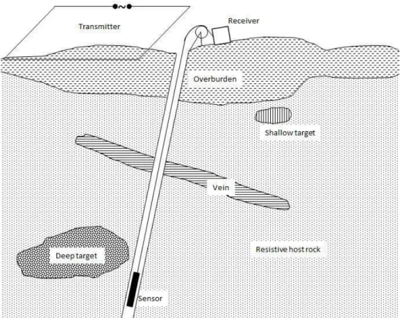
In a typical BHTEM configuration, shown in Figure 1.1, there are a large transmitter loop, a winch and a receiver on the surface, and a sensor connected with the receiver through a cable, is lowered in the borehole.

(20)

Figure 1.1 Geoelectric cross section illustrating the application of the BHTEM in exploring deep targets (adapted from Dyck, 1981).

The basic principles of the BHTEM are the same as surface time domain EM. A strong direct current is injected into the transmitter loop for a certain time until all turn-on transients have vanished, giving the primary electric field; then, the current through the transmitter loop is cut off, and the primary electric field has been changed abruptly. According to Faraday's law, the abrupt change will induce eddy currents in nearby conductors, because of ohmic losses these eddy currents dissipate gradually. The dissipation of these eddy currents, in turn, induces a decaying magnetic field which is the secondary magnetic field. It is the magnetic induction 𝐵 or its time rate 𝑑𝐵 𝑑𝑡⁄ of the secondary magnetic field recorded by the receiver. At present all systems effectively perform 3-axis component measurements, one axial component (A) and two transverse components (U and V), as shown in Figure 1.2.

(21)

Figure 1.2 The three components (A, U, V) recorded by the sensor. A—parallel to the trajectory of the borehole (coaxial component), U—in the same vertical plane as A and perpendicular to A, V—perpendicular to A and U in a right-hand coordinate system.

The BHTEM method shares the same principle with other TEM methods (airborne TEM, and ground TEM), however, challenges exist in processing BHTEM data because of the noise. Apart from common noises encountered airborne TEM and ground TEM, such as motion induced noise, cultural noise and sferics (Macnae et al., 1984), the hostile environment in a borehole, especially in deep holes, there are some additional sources of noise as thermal noise at high temperature, flowing liquid in well, and the rotation of the sensor. These problems of BHTEM motivate us to develop an effective and efficient denoising method for BHTEM data.

1.3 Objectives of research

With the financial support of FRQNT (Fonds de recherche, Nature et Technologies du Québec), the main goal of this Ph.D. research is to develop an efficient denoising tool dedicated to BHTEM measurement for deep mine exploration. The research has been carried out in close collaboration with Abitibi Geophysics Inc. Therefore, our work is focused on providing an effective and easy to use tool for field geophysicists

(22)

to improve data quality, thus improve the accuracy of interpretation. Three specific objectives have been accomplished through this research:

a) As everything can give an electromagnetic signal in response to an induced electromagnetic field, identify the main sources of noise in a typical deep mine environment is one of the objectives of this Ph.D. study.

b) The second specific objective is to develop new noise elimination algorithms. A strategy for improving BHTEM data quality has been developed. The strategy involves denoise raw data by a discrete wavelet transform; moreover, distorted transients are identified by correlation analysis, and then these distorted transients are corrected.

c) Develop an interface for denoising BHTEM raw data in the Matlab environment, in order to transfer the denoising tool to the industrial partner. 1.4 Thesis outline

This thesis has been divided into five chapters of which Chapter I is the general introduction.

Chapter II summarizes the theory of the signal processing methods used in the frame of this Ph.D. research.

Chapter III describes briefly on the data acquisition in tunnels of a deep mine. As an effort to investigate influences of the environment on EM measurements, the recordings are analyzed using both the Fourier and the wavelet transform integrating information from seismic records, blasting, fluctuation in powerlines.

Chapter IV focus on the development of a new denoising method for BHTEM data based on DWT. Results of using the method to denoise synthetic and field BHTEM data are presented in detail.

(23)

CHAPTER II

METHODS AND THEORY

2.1 Wavelet transform

Basic concepts and theory of the wavelet transform (WT) described in this section mainly refer to Daubechies (1992), Chui (1992), Mallat (1999), Percival and Walden (2006).

The wavelet transform (WT) has often been compared with the Fourier transform (FT) and can be considered as an improved, localized equivalent of it. They share the same principle, which is that all signals can be decomposed into a superposition of functions, called basis functions. These basis functions possess certain properties: simple, harmonic, symmetry, orthogonal. Therefore, the process of analysis based on the decomposition is simplified. After the processing, the signal can be reconstructed through a process called inverse transformation (IWT, and IFT). In the case of FT, the signal is decomposed into an integral or sum of trigonometric functions with different frequencies. Each trigonometric function represents a frequency component of the original signal. This facilitates the analysis of a signal in the frequency domain. It shows how much of the signal lies within a specific frequency, however, this is at the cost of time information. In other words, it does not tell us when an event occurs in the signal. The WT remedies the deficiency of the FT by changing the basis function from trigonometric- functions to mother wavelets, which are a waveform of limited duration, zero average value, and nonzero norm. The advantage of using wavelets as

(24)

the basis functions is that it enables one to study features of the signal locally with a detail matched to their scale (Kumar and Foufoula-Georgiou, 1994). In other words, the WT allows analyzing a time series at different scales without sacrificing time resolution.

2.1.1 Continuous wavelet transform (CWT)

Using FT to analyze the frequency content of a time series, the basis function is explicitly defined as the trigonometric function, which has an infinite duration as defined in equation (2.1). ℱ𝑓(𝜔) = 1 √2𝜋∫ 𝑓(𝑡)𝑒 −𝑖𝜔𝑡_𝑑𝑡 ∞ −∞ . (2.1)

The selection of trigonometric function as the basis function results in an inherent limitation of the FT: it provides high resolution in frequency without offering any time information about the signal. If the signal is stationary, which means the frequency content of the signal does not change over time, the FT would be a good choice. For non-stationary signals, whose frequency content changes over time, the FT does not provide enough information to characterize the signal.

In order to provide time-localized information in the frequency domain, a windowing function is added to the Fourier transform (Gabor, 1946). It is called short-time Fourier transform (STFT):

𝑆𝑇𝐹𝑇𝑓(𝜔, 𝜏) = ∫ 𝑓(𝑡)𝑤(𝑡 − 𝜏)𝑒∞ −𝑖𝜔𝑡_𝑑𝑡

−∞ . (2.2)

The introduction of the windowing function, w(t), splits the signal that changes with time into small segments, and it assumes the signal is stationary in each segment. This technique has remedied the deficiency of the FT to a certain degree. However, once w(t) is chosen, the size of the window is fixed. This is the main disadvantage of the STFT in dealing with non-stationary processes, which requires varying window size to give reasonable resolution for both time- and frequency-localized events. This

(25)

is what exactly wavelet transform provides. The WT uses a wide window for low-frequency events and a narrow window for high-low-frequency contents. Figure 2.1 illustrates the time resolution difference as frequencies ascend for the Fourier transform and the wavelet transform. For the FT, the resolution uniform for all frequencies. However, in the WT, the time resolution increases with the increase of the frequency.

Figure 2.1 Resolution difference in time between the STFT (left) and the WT (right): (a) uniform tiling; (b) scale adaptive tiling.

The continous wavelet transform (CWT) of a time series with finite energy is defined as:

𝐶𝑊𝑓(𝑎, 𝑏) = ∫ 𝑓(𝑡)𝜓_−∞∞ 𝑎,𝑏(𝑡)𝑑𝑡. (2.3)

Here a and b are scale and translation parameters. The function ψa,b(t) is called the

mother wavelet, which does not have a general formulation, but must meet the following two conditions:

∫ 𝜓(𝑡)𝑑𝑡 = 0_−∞∞ , (2.4) 𝐶𝜓 = ∫ |ℱ𝜓(𝜔)| 2 𝜔 0 −∞ 𝑑𝜔 = ∫ |ℱ𝜓(𝜔)|2 𝜔 𝑑𝜔 ∞ 0 < ∞. (2.5)

The symbol ℱ indicates the Fourier transform. The most important operation implemented in equation (2.3) is scaling and translating a mother wavelet with the help of the scale and translation parameters (a and b, respectively). A wavelet family

(26)

has wavelets of the same shape, but various dilation levels and positions defined as below:

𝜓𝑎,𝑏(𝑡) =_√𝑎1 𝜓 (𝑡−𝑏_𝑎 ) 𝑎, 𝑏 ∈ 𝑅; 𝑎 > 0. (2.6)

After the CWT, a set of coefficients is obtained. Processes, such as removing certain frequency contents from the signal, can be operated on these coefficients. Since the transform is isometric, i.e. it preserves the energy of the signal, the transformation is reversible. The reverse continuous wavelet transform (iCWT) is defined as:

𝑖𝐶𝑊𝑓(𝑡) =_𝐶1 𝜓∫ ∫ 1 𝑎2𝐶𝑊𝑓(𝑎, 𝑏)𝜓𝑎,𝑏(𝑡)𝑑𝑎𝑑𝑏 ∞ −∞ ∞ −∞ . (2.7)

In order to make a comparison between FT, STFT, and WT, two time series of signals are generated. One is a stationary signal (𝑠1) and another is a non-stationary

signal (𝑠2). The 𝑠1 is a sinusoid signal consisted of three frequency components:

30Hz, 50Hz, and 80Hz. The non-stationary signal 𝑠2 is composed of two frequency

components: 50Hz and 80Hz. Except that the 50Hz component is present everywhere in the signal 𝑠2, the 80Hz component only occurs between 400ms and 600ms. Figure

(27)

Figure 2.2 Stationary signal 𝑠1 (a) and non-stationary signal 𝑠2 (b) in the time

domain.

Those two signals were then processed by three transformations one by one, namely FT, STFT, and WT. Figure 2.3 presents the results of FT for the two signals. In both cases, the frequency components are identified successfully but it fails to show the time-varying features in the non-stationary signal 𝑠2, because all time information is

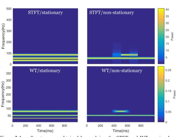
last after the transformation. This is a severe weakness of the FT in dealing with non-stationary signals. To overcome this weakness the STFT and WT are available. In Figure 2.4, we can see for the stationary signal both the STFT and WT have correctly detected the three frequency components in the signal; however, the STFT gives uniform resolution for all freqeuncy components, because the resolution is pre-decided by the selection of the window size. Comparatively, the WT offers different resolution for different frequencies. Moreover, the WT provides much better time precision for non-stationary signals than the STFT.

(28)

These results (Figure 2.4) show that the WT is much better than the other two methods, especially for non-stationary signals. In reality, geophysical signals are often non-stationary.

(29)

Figure 2.4 Spectrograms obtained by applying the STFT and WT on signals 𝑠1

and 𝑠2.

2.1.2 Discrete wavelet transform (DWT)

Since the scale and translation parameters (a, b) are continuous, information provided by the CWT is highly redundant, which makes the CWT computationally inefficient. It is used usually for analytic purposes. To reduce the redundancy, parameters a and b are discretized, and often use dyadic values as below:

𝑎 = 2𝑗_{;𝑏 = 𝑘 ∙ 𝑎 = 𝑘 ∙ 2}𝑗_{𝑗, 𝑘 ∈ 𝑍.} _(2.8)

Where j is called the decomposition level, which controls the dilation; k controls the translation. Substitute equation (2.8) into equation (2.6), the wavelet family becomes:

𝜓𝑗,𝑘(𝑡) =_√21_𝑗𝜓(𝑡−𝑘∙2

𝑗

2𝑗 ). (2.9)

(30)

Figure 2.4 Spectrograms obtained by applying the STFT and WT on signals 𝑠1

and 𝑠2.

2.1.2 Discrete wavelet transform (DWT)

Since the scale and translation parameters (a, b) are continuous, information provided by the CWT is highly redundant, which makes the CWT computationally inefficient. It is used usually for analytic purposes. To reduce the redundancy, parameters a and b are discretized, and often use dyadic values as below:

𝑎 = 2𝑗_{;𝑏 = 𝑘 ∙ 𝑎 = 𝑘 ∙ 2}𝑗_{𝑗, 𝑘 ∈ 𝑍.} _(2.8)

Where j is called the decomposition level, which controls the dilation; k controls the translation. Substitute equation (2.8) into equation (2.6), the wavelet family becomes:

𝜓𝑗,𝑘(𝑡) =_√21_𝑗𝜓(𝑡−𝑘∙2

𝑗

2𝑗 ). (2.9)

(31)

𝐷𝑊𝑓(𝑗, 𝑘) = ∫ 𝑓(𝑡) ∙ 𝜓_−∞∞ 𝑗,𝑘(𝑡)𝑑𝑡= 〈𝑓, 𝜓𝑗,𝑘〉. (2.10)

In DWT, the wavelet is selected to form an orthonormal basis for functions with finite energy. This implies that all such functions can be approximated by a linear combination of the wavelets (Kumar and Foufoula-Georgiou, 1994):

𝑓(𝑡) = ∑∞𝑗=−∞∑∞𝑘=−∞〈𝑓, 𝜓𝑗,𝑘〉𝜓𝑗,𝑘(𝑡). (2.11)

The two indices j and k indicate scale and position, respectively. Hence, DWT has the time-scale, or time-frequency, localization ability.

Defining J as the decomposition level, the equation (2.11) can be broken into two parts:

𝑓(𝑡) = ∑ ∑∞ 〈𝑓, 𝜓_𝑗,𝑘〉𝜓_𝑗,𝑘(𝑡)

𝑘=−∞ 𝐽

𝑗=−∞ + ∑∞𝑗=𝐽+1∑∞𝑘=−∞〈𝑓, 𝜓𝑗,𝑘〉𝜓𝑗,𝑘(𝑡). (2.12)

The first part is called details of the function. The second part is called the approximate of the function.

To simplify the process the scale function 𝜙𝑗,𝑘(𝑡) is introduced, and it can be defined

analogically to the wavelet function 𝜓𝑗,𝑘(𝑡) in equation 2.9:

𝜙_𝑗,𝑘(𝑡) = 1

√2𝑗𝜙(

𝑡−𝑘∙2𝑗

2𝑗 ). (2.13)

Details on finding the scale functions can be found in Mallat (1989). With the scale function, the second sum on the right side of the equation (2.12) can be rewritten as:

∑∞𝑗=𝐽+1∑∞𝑘=−∞〈𝑓, 𝜓𝑗,𝑘〉𝜓𝑗,𝑘(𝑡)= ∑𝑘=−∞∞ 〈𝑓, 𝜙𝐽,𝑘〉𝜙𝐽,𝑘(𝑡). (2.14) Therefore: 𝑓(𝑡) = ∑ ∑∞ 〈𝑓, 𝜓_𝑗,𝑘〉𝜓_𝑗,𝑘(𝑡) 𝑘=−∞ 𝐽 𝑗=−∞ + ∑∞𝑘=−∞〈𝑓, 𝜙𝐽,𝑘〉𝜙𝐽,𝑘(𝑡). (2.15)

As a result of DWT, the signal is decomposed into detail (𝐷𝑗,𝑘) and approximate

(32)

𝐷𝑗,𝑘 ≡ ∫ 〈𝑓, 𝜓_−∞∞ 𝑗,𝑘〉𝜓𝑗,𝑘(𝑡)𝑑𝑡

𝐴_𝑗,𝑘 ≡ ∫ 〈𝑓, 𝜙_−∞∞ 𝑗,𝑘〉𝜙𝑗,𝑘(𝑡)𝑑𝑡

. (2.16)

Please note that the equation (2.16) is used to calculate coefficients of single scale decomposition. To calculate wavelet coefficients for a certain decomposition level, multiple scale decomposition mechanism must be used. Figure 2.5 illustrates the DWT process for multiple decomposition levels:

1. At first, the signal is fed to a highpass filter and a lowpass filter producing the level one detail coefficients and approximation coefficients, respectively. 2. The detail coefficients are kept unchanged; the approximation coefficients are

fed to another highpass filter and another lowpass filter producing level two detail coefficients and approximation coefficients. This process is repeated until the desired decomposition level is reached.

3. The decomposition process is a down-sampling process by a factor of two. To reconstruct the signal the coefficients are upsampled.

Figure 2.5 Implementation of the DWT in terms of filter banks (the downward arrow indicates down-sampling by a factor of two) (Percival and Walden, 2006).

(33)

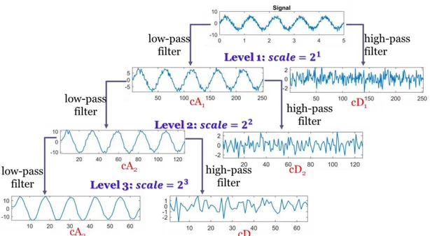
Figure 2.6 is an example showing a signal is decomposed to level 3 with the DWT, which we can summerize as below.

a) Detail coefficients (𝑐𝐷𝑖) store high-frequency features of the signal; and

approximation coefficients (𝑐𝐴𝑖) show low-frequency components of the

signal.

b) Higher decomposition level means larger scale value; features extracted from the signal or the approximation coefficients of the previous level to the detail coefficients have lower frequencies, and vice-versa.

Figure 2.6 A signal is decomposed to level 3 with the DWT. 2.1.3 Selection of a wavelet

There is a number of wavelet families, such as Haar, Daubechies, Symlets, Coiflets, Biorthogonal, Meyer, Gaussian, Mexican hat, Morlet, Shannon, Frequency B-Spline, Complex Morlet and Fejer-Korovkin wavelets (see wavlet Toolbox of MATLAB). Users have to decide first which wavelet is suitable for their application: CWT or DWT. If the goal of the application is to perform a detailed time-frequency analysis,

(34)

then the CWT is a good choice; however, if the application is about general denoising, compressing, or feature detecting, DWT is superior to CWT (https://www.mathworks.com/help/wavelet/gs/continuous-and-discrete-wavelet-transforms.html). As already mentioned, the CWT provides a highly redundant representation of a signal, the cost of computing and storage of CWT coefficients is much greater than for the DWT. A detailed comparison between the CWT and the DWT can be found in the documentation of wavelet transform in Matlab.

Unfortunately, there is no straightforward method to choose an appropriate wavelet. In fact, the characteristics of the signal and the purpose of the application influence which wavelet should be used. We summarized some general rules from the documentation of the wavelet toolbox in Matlab:

a) In time-frequency analysis, analytic wavelets, such as generalized Morse wavelet, analytic Morlet wavelet, and bump wavelet, are a good choice. b) If the application requires preserving the energy of the signal, an orthogonal

wavelet must be used, because orthogonal transforms preserve energy. In this case, wavelets like coiffet, daubechies, and haar are a good choice.

c) Although orthogonal wavelets are most commonly used, the wavelet’s orthogonality restricts the type of decomposition and reconstruction filters. Non-orthogonal transforms, on the contrary, have fewer restrictions on the type of filters; therefore, filters with finer frequency resolution are available (Fargues et al., 1997). So if a high resolution in the frequency domain is needed for the application, non-orthogonal wavelets can be considered.

d) To detect features, the support, which indicates the non-zero interval of a wavelet, must be chosen accordingly: small support for closely spaced features. Wavelets with large support can be used if features in the signal are sparsely spaced.

(35)

e) In case of compression, consider using biorthogonal wavelets. Biorthogonal wavelets are symmetric and have linear phases. They have two pairs of scaling function-wavelet: one pair is for analysis, and the other one is for synthesis. This feature of biorthogonal wavelets is very useful in compressing an object.

f) If the application is to denoise signals, orthogonal wavelets are a good candidate. An orthogonal transform preserves energy and does not color white noise.

Although the choice of basic wavelet types can be guided by these guidelines, there is no concrete criterion for us to choose a specific wavelet for a specific application. Proceeding by trials and errors is the only way. We tried a lot of wavelets in our study, such as the harr wavelet, the daubechies wavelet family, and the symlet wavelet family. Finally the ‘sym5’ wavelet of the symlet wavelet family is chosen in our study (details are discussed in Chapiter IV).

2.2 Complementary methods

Our denoising method development begins with synthetic signals and known noise. After using DWT to process the synthetic signal, in some cases we have observed that there are still residual perturbations remaimed. Since in a time-domain geophysical survey, as borehole transient electromangetic measurement (BHTEM), the secondary magnetic field (B) and/or its time rate (dB/dt) is recorded after the primary electric field disappeared, the decay of the secondary magnetic field is often estimated by an exponential function (Equation 2.17) (Nabighian and Macnae, 1991). The importance is that the decay time constant is reverse to the exponential decay constant. Larger decay constant (small time constant) makes the transient signal vanish much more rapidely than small decay constant (large time constant); and the time contant is one of important characteristics used in the mineral exploration to discrimining good or bad conductor. A stable decay can ensure a good estimation of

(36)

the time constant. Therefore, the residual perturbation in the signal can lead to misinterpretation of data. In order to further improve the data quality, we introduce a curve fitting method dedicated to simple date sets, perhaps mostly for theoritical tests purposes.

For a practical time domain electromagnetic (TEM) survey, the measurement is often repeated many times at each survey point. The correlation method is therefore further developed to eliminate residual radom noises. Those two methods are described below.

2.2.1 Curve fitting technique (CFT)

Although the induced polarization (IP) effect is always present in all electromagnetic (EM) surveys when polarizable minerals, such as clays, massive and disseminated sulphides, are present; however, the IP signal is low and completely overlapped with the inductive effect. In addition, Smith and West (1989) pointed out that the in-loop EM system is the optimal configuration to excite the airborne IP response including negative transients in mid to late times over resistive grounds, from bodies of modest chargeability under condition of layered structure or homogenous half space. The fact that the most of borehole EM surveys use out-off loop EM system, and whole space and highly inhomogeneous milieu are involved. It is impossible to characterize the IP effect in borehole EM (personnal communication with senior geophysicists of companies), therefore, we ignore IP effect on exponential transient decay model in this study. We apply the exponential function below as our model to implement the fitting process to reduce the residual perturbation after DWT process.

𝑠(𝑡) = 𝛼𝑒−𝑡 𝜏⁄ _, _(2.17)

where α and τ are parameters to be determined. They denote the gain parameter and the time constant of the conductor, respectively. They are calculated according to the linear least-squares criterion. Take the natural logarithm of both sides of Equation (2.17), we got:

(37)

𝑙𝑛𝑠(𝑡) = 𝑙𝑛𝛼 +_−𝜏1 𝑡. (2.18)

Let 𝑦 = 𝑙𝑛𝑠(𝑡), 𝑝1 = 𝑙𝑛𝛼, and 𝑝2 =_−𝜏1, then we have

𝑦 = 𝑝₁ + 𝑝₂𝑡. (2.19)

Suppose 𝑦̃ is the fitted data, then the residual of the ith (i=1,2,3,…,n) data is defined as

𝑟𝑖 = 𝑦𝑖− 𝑦̃𝑖 = 𝑦𝑖 − (𝑝1+ 𝑝2𝑡𝑖). (2.20)

Sum the square of residuals of all data, we got 𝑆 = ∑𝑛 𝑟_𝑖2

𝑖=1 = ∑𝑛𝑖=1(𝑦𝑖− (𝑝1+ 𝑝2𝑡𝑖))2. (2.21)

Because the purpose of the least-square process is to minimize S, the parameters to be determined are solutions of the equation set formed by differentiating the Equation (2.21) with respect to each parameter, and setting the result to zero:

𝜕𝑆 𝜕𝑝1= −2 ∑ 𝑥𝑖(𝑦𝑖 − (𝑝1𝑥𝑖 + 𝑝2)) 𝑛 𝑖=1 = 0 𝜕𝑆 𝜕𝑝2= −2 ∑ (𝑦𝑖 − (𝑝1𝑥𝑖 + 𝑝2)) 𝑛 𝑖=1 = 0 . (2.22)

Solve equation set (2.22):

𝑝₁ =𝑛 ∑𝑛𝑖=1𝑥𝑖𝑦𝑖−∑𝑛𝑖=1𝑥𝑖∑𝑛𝑖=1𝑦𝑖

𝑛 ∑𝑛_𝑖=1𝑥_𝑖2

𝑝2 =_𝑛1(∑𝑛𝑖=1𝑦𝑖 − 𝑝1∑𝑛𝑖=1𝑥𝑖)

. (2.23)

Therefore we get the two unknow parameters in Equation (2.17): 𝛼 = 𝑒𝑝1

𝜏 = −_𝑝1

2

(38)

To constrain the fitting result, perturbed segments in the data are identified and excluded from the fitting process. These segments are determined through the following steps:

1. Find extrema. The perturbation of signal represents local peaks or valleys in the data. The first step is to determine the location of these extremes on the decay curve.

2. The width of each peak and valley is then estimated by its half-prominence. The prominence of a peak measures how much the peak stands out due to its intrinsic height and its location relative to other peaks (Source: Matlab). All these parameters can be easily obtained by using the built-in function findpeaks in Matlab. Figure 2.7 explains how to decide the prominence of a peak.

Figure 2.7 Definition of the prominence of a peak. Vertical arrows indicate the prominence of the peak. (source:

https://commons.wikimedia.org/wiki/File:Prominence_definition.svg)

3. Exclude points from the fitting process. Points fall within the range of half-prominence of the peak are considered as being contaminated by residuals, thereby excluded from the fitting process and replaced later by values from the fitting result.

(39)

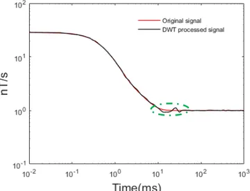
The following example shows how this method is implemented. Figure 2.8 presents the result of denoising with the DWT, but perturbations caused by noise residuals still exist in the result. In order to use the fitting method, we first find out the peaks/valleys in the denoised signal as shown in Figure 2.9. the width of these peaks/valleys can be estimated with the help of half-prominence. To reduce their impact on the fitting result, points fall in range of half-prominence around the peak/valley are excluded from the fitting process. Figure 2.10 shows the CFT smoothes the perturbations caused by noise residuals effectively.

(40)

Figure 2.9 Peaks/valleys located in the DWT denoised signal.

Figure 2.10 Comparison between the DWT denoised result and DWT+CFT processed result.

2.2.2 Correlation analysis and stacking

Generally, in a BHTEM field survey, the measurement is repeated many times at each survey point. Then, these measurements are stacked into one record in an effort to eliminate random noise. Since repeated measurements are at the same survey point,

(41)

they are basically recording signals from the same source. The response of geological bodies to primary electromagnetic fields will not change in repetitve measurements, but random noises will change. As we mentioned in section 1.3, during the measurement of BHTEM the sensor may rotate and/or vibrate because of the liquid flow or obstacles in the borehole. This rotation and/or vibration will be one type of source of noises to the measurement. Using conventional stacking methods one can reduce random noise, but when there is an acute noise signal, it can skew the neighboring data. This is why we first use DWT method to process the raw data, and then do correlation analysis in order to distinguish the geological response versus noises.

Figure 2.11 illustrates a cycle of recording in TEM method. A cycle includes four transients: two on-time transients and two off-time transients.

Figure 2.11 Basic principles of measurement of the TEM method. The red line indicates the current in the transmitter loop, and the blue line shows the signal recorded by the sensor.

Based on this recording mechanism, we can use correlation to identify the distorted transients. The Pearson correlation coefficient is chosen because of its invariance, i.e., the coefficient is not affected by separate changes in the two variables in location and

(42)

scale. For example, if one variable X is changed to 𝛼𝑋 + 𝛽, and another variable Y is changed to 𝜆𝑌 + 𝛾, where 𝛼, 𝛽, 𝜆, and 𝛾 are constants, and 𝛼, 𝜆 > 0, the correlation coefficient will not be changed. The coefficient between two variables X and Y is calculated by the formula:

𝜌𝑋,𝑌 =𝑐𝑜𝑣(𝑋,𝑌)_𝜎

𝑋𝜎𝑌 , (2.18)

where, 𝑐𝑜𝑣(𝑋, 𝑌) calculates the covariance between variables X and Y; σX and σY is

the standard deviation of X and Y, respectively.

The correlation coefficient calculated by equation (2.18) ranges from -1 to 1. The value of 1 means there is a perfect linear relationship between the two variables. The value of -1 implies that the two variables still have a linear relationship, but they change in an opposite direction, in other words, one variable decreases as the other one increases. When the correlation coefficient equals to zero, there is no linear correlation between the two variables. For example, if we have a five-transients record, and we compute the Peason coefficients between them. We will get a diagonal matrix shown in Table 2.1. From these values we can conclude that the transient-2 has a bad correlation with other transients, it must be distorted.

Table 2.1 Pearson coefficients between five transients.

transient 1 2 3 4 5 1 1.00 0.65 0.95 0.94 0.99 2 0.65 1.00 0.68 0.70 0.64 3 0.95 0.68 1.00 0.97 0.98 4 0.94 0.70 0.97 1.00 0.92 5 0.99 0.64 0.98 0.92 1.00

After the distorted transient is identified with the help of correlation analysis, it is replaced by linear interpolation using other transients. Figure 2.12 shows the distorted transient (red line) is replaced by interpolation (dashed blue line). The interpolation is carried out sampling by sampling, i.e., we first take the first sampling of each

(43)

transient which is not distorted to do a linear interpolation to get the first sampling to replace the first sampling of the distorted transient. Then we repeat this process on other samplings until the entire distorted transient is replace.

Figure 2. 12 Schematic diagram illustrating the process of replacing distorted transient with interpolation.

2.2.3 Stacking

Stacking is a fundamental and essential step in time series of geophysical data processing. The goal of stacking is to improve the signal-to-noise ratio. After decades of development many stacking techniques have been developed. The most simple one is the average stacking method. For each survey point, it adds up all isochronous values and the sum is then divided by the number of values to get the stacked results, as defined by Equation (2.19):

𝐴𝑡 =_𝑁1∑𝑁𝑘=1𝑎𝑖. (2.19)

𝐴_𝑡 is the stacked result of channel time t. And 𝑎𝑖 is the sample value of the ith

measurement of the corresponding channel. N is the total repeated measurement times. In this stacking method a uniform weight is used for all measurement. This makes the method very easy to understand and to use, but it cannot be used to deal with data with drift. To remove linear drift Mark Halverson developed a method called Halverson stacking in 1960s. Three half periods are engaged each time in the stacking process (Kingman et al., 2004), and weights for these three half periods are:

(44)

1 4, −

1 2,

1

4. So, if there are four half periods in the data set, then the weight for each half

period can be decided as follows (Kingman et al., 2004):

( 1 4 − 1 2 1 4 + −1₄ 1₂ −1₄) ∙ 1 2 = [ 1 8 − 3 8 3 8 − 1 8]. (2.20)

Weights for data set with more half periods can be obtained similarly. A general formula for weights when there are more than four half periods in the data set is below (Kingman et al., 2004):

[1,−3,4,−4,4,−4,⋯,4∙(−1)𝑛−3_,3∙(−1)𝑛−2_,1∙(−1)𝑛−1_]

4∙(𝑛−2) , (2.21)

where, n is the total number of half periods in the data set.

The Halverson stacking method is used in this study. To compare the results stacked from different raw data (original raw data, DWT denoised raw data, and DWT denoised plus distorted transients corrected raw data), we will use Halverson stacking in our study.

(45)

CHAPTER III

CHARACTERISATION OF EM NOISES IN DEEP MINING TUNNELS

3.1 Introduction

Every geophysical datum consists of two parts: information related to the target, and all other regarded as noise. Commonly encountered noise sources in EM measurements can be categorized as man-made noise and natural noise.

On surface, man-made noises come mainly from power distribution grid. The frequency of this kind of noise is usually highly stable and its features are easily determined. By contrast, the natural noise is much more complicated and difficult to remove. One major source is sferics, and it is not uniformly distributed throughout the measurement bandwidth but typically concentrated in the high frequency part (Macnae et al, 1984). Energy in the 5 Hz – 25k Hz range is primarily due to sferics, which are natural transients generated by lighting discharges; and the natural EM noise below about 6 Hz is mainly of geomagnetic and ionospheric origin. In addition, natural noise fields may change from place to place and from time to time, and therefore are more difficult to handle. Toward the Earth interior but near the surface, the conductive overburden in the survey area has a strong effect on the EM field (Macnae et al, 1984). It may greatly weaken the penetration of electromagnetic waves. Deep in underground tunnels, the shielding effect of the rock formation may reduce the noise effects of some electromagnetic fields on the ground; however, due

(46)

to the difficulty of entering the underground tunnel, there is a lack of understanding of the noise in such deep environment. Thanks to the financial support of the FRQNT (Fond de Recherche Naturel et Technologies du Québec), our industry partner (LaRonde Mine of Agnico Eagle) allowed us to install 5 electromagnetic signal recorders at 5 places in 3km deep underground tunnels. Those five places represent typical deep mining environment, quiet and noise-concentrated areas (detailed information in Table 3.1). This chapter aims at the characterization of underground recorded EM signals.

3.2 A brief description of LaRonde Mine

At about 47 kilometers east of Rouyn-Noranda City, the LaRonde Mine is an Au-rich volcanogenic massive sulfide (VMS) deposit. The deposit is a huge subvertical tabular of east-west orientation. It was first discovered in 1976 by Dumagami Mines Ltd., and first achieved commercial production in 1988. It is now fully owned by Agnico Eagle Ltd. Among the ten deepest mines in the world, the LaRonde deposit is one of the most important VMS deposits hosted in the Abitibi greenstone belt, and it is the largest Au deposit currently mined in Canada (Mercier-Langevin et al., 2007). The mine has produced more than 5 million ounces of gold along with valuable by-products and still has 2.6 million ounces of gold in proven and 15 million tonnes grading 5.39 grams of gold per tonne probable reserves as of the end of 2017 (Agnico Eagle website). The production of the mine now mainly comes from deep ore bodies; and the exploration is directed toward great depth and the periphery as shown in Figure 3.2.

(47)

Figure 3.1 Geological map and location of the LaRonde mine (Source : modified

from interactive carte of SIGEOM, MERNQ,

(48)

Figure 3.2 Composite longitudinal section of the LaRonde mine (Source : https://www.agnicoeagle.com/English/operations-and-development-projects/operations/laronde/maps-and-surveys/default.aspx).

3.3 Geological setting of LaRonde Mine

The LaRonde mine is located near the southern boundary between the Abitibi Sub-province and the Pontiac Sub-Sub-province, within the Superior Province of the Canadian Shield (Gosselin, 2005). It is about 4km in the north of an important regional geological structure – the Cadillac-Larder Lake Fault (CLLF), which is indicated as the broken red line in Figure 3.1.

During late Archean orogenesis, accompanied by large-scale north-south compression and dextral transpression tectonic events (Card 1990), the lithological sequences near

(49)

the CLLF were sub-verticalized, dipping toward the south. From the north to the south three geological formations around the LaRonde Mine are: (1) the Kewagama Group formed by thick band of interbedded wacke; (2) Blake River Group, which is a volcanic assemblage and the host of all known economic mineralisation of the LaRonde mine; (3) the Cadillac Group which is made up of thick band of wacke interbedded with politic schist and minor iron formation (Gosselin, 2005).

The key question for the futur development of the LaRonde Mine is: how much economic minerals remain unexploited under the depth of 3km? Where comes out the importance to do some geophysical surveys in order to estimate the mineral potential around known mineralization. Among conventional geophysical methods, the time domaine electromagnetic method is widely applied to explore volcanogene massive sulfides minerals. One of the important factors affecting the efficiency of this method is the ratio of the signal to noise. Several potential noise sources could exist in a deep mine, such as Schumann remanence (7.83 Hz) ; VLF (Very low frequency) (3 – 30 kHz); EM field resulted from coupling between machine vibration and EM field (attenuate quickly with distance) ; power lines (between 50 and 60 Hz) and communication cables (high frequency), but we lack of knowledge on them, especially in an active deep mining environment. We therefore decided first to record noises in deep tunnels of the LaRonde mine.

3.4 Data acquisition

3.4.1 Zonge Electromagnetic Network (ZEN) receiver

The device we used to collect data in the tunnels of the LaRonde mine is Zonge Electromagnetic Network (ZEN) receiver (Figure 3.3), which is a product of Zonge International Inc. ZEN receiver is a broadband, high-resolution, and multi-function digital receiver for acquisition of controlled- and natural-source geo-electric and EM data. It has up to 6 channels and it is expandable. The frequency range of the receiver is from DC up to 1024 Hz. The device is small in size (27 × 24 × 13 𝑐𝑚) and very

(50)

light (3Kg with 6 channels, without battery and meter/connection panel) (source :. http://zonge.com/instruments-home/geophysical-data-acquisition-systems/distributed-em-systems/). The magnetic sensor we used in this survey is ANT/6 of Zonge International Ltd. The sensor uses feedback amplifier technology and including carefully designed mu-metal cores. It is a multipurpose coil with low noise level:100 𝜇𝛾 (100 fT) per √𝐻𝑧 at 1 Hz, 100 𝜇𝛾 (100 fT) per √𝐻𝑧 nominal>1 Hz. The length of the sensor is 91.0 cm, and its diameter is 4.8 cm. The weight of the sensor is around 3.2 kg. The frequency range of the sensor is 0.1—10240 Hz (Source: http://www.zonge.com/legacy/MagSensors.html).

Figure 3.3 The Zonge Electromagnetic Network (ZEN) receiver (Source: Zonge International Inc.).

(51)

3.4.2 Sites of recordings

With the help from geologists of LaRonde Mine, five representative places have been chosen at 3000 m depth. They are: 1) in a relatively quiet area (site #1); 2) near a conveyor, and under a crusher, which crushes large minerals (site #2); 3) near the massive sulfide mineralization zone and a loading station (site #3); 4) under the power supply center (site #4); and 5) beside a drilling site (site #5). These sites are indicated as circled numbers in Figure 3.4. The characteristics of the sites are summarized in Table 3.1.

Table 3.1 Description of all recording sites. The five sites are all located in the tunnels at 3000m depth.

site description _{(Apr 12, 2018)}Start time _{(Apr 13, 2018)}End time recording Total time

Sampling rate

1 No mining _activity 09:40AM 07:56AM 22h 16m 1024

2 Nearby a mineral conveyor

Crusher above 10:11AM 08:22AM 22h 11m 1024

3 Nearby a loading _station 10:51AM 08:56AM 22h 05m 1024 4 Under a power _station 11:29AM 09:19AM 21h 50m 1024

5 Nearby a drilling site (Less than

(52)

Figure 3.4 Locations of the five data acquisition sites (scale: 1:2000). 3.4.3 Recorded signals

There are 6.11 gigabytes electromagnetic data recorded during more than 22 hours. For better associating changes in the EM signals with underground mining activities, the operation period of mining equipment (drilling, crusher, and convoyor etc.) is considered. Operation hours for the drilling site that is near the data acquisition site #5 are from 08:00:00 to 15:00:00 on April 12, 2018, and from 20:00:00 on April 12, 2018 to 03:00:00 on April 13, 2018. In addition, Figure 3.5 tells the electrical current variations in the conveyor near the data acquisition site #2. All data acquisition sites were blocked for the measurement, therefore no traffic presented at all sites during the period of recording. Two blasting events took place between 17:43:28.992 and 17:43:37.661, 05:19:24.873 and 05:19:34.437. The first blast happened near 380 m above site #2, while the 2nd is 50 m in the East-North of site #2. However, we do not

(53)

have GPS signal in the tunnels; therefore, all recordings are not synchronized. Consequently, not only did the five receiver start and end recording at different time, but each channel of a specific receiver had different start and end time. We have not yet found an appropriate way to locate such a short period of time in our recordings. These blasts are thus not considered as a noise source.

Figure 3.5 The current in the conveyor varies with time. 3.5 Recorded time series

At each site, four components of electromagnetic field are recorded. They are: the horizontal electric field (Ex and Ey), and magnetic field (Hx and Hy).

Figure 3.6 and Figure 3.7 present time series from all acquisition sites. The behavior of the electric components is a bit abnormal. Since noises are not polarizable, which means they are mostly random distributed (Gaussian distribution), the average value should be around zero, like we have observed in magnetic field components (Hx and Hy). In addition, the behavior of the Ex and Ey should be alike, as Hx and Hy, but it is not. The reason of these phenomena is not clear yet, they may caused by the self potential effect, which is usually a result of charge separation in some minerals, or natural flow of the conducting liquid through the rocks. In spite of these unusual

(54)

behaviors of Ex and Ey, we will still present analysis results of Ex and Hy in this chapter. But in future works, we will focus on the magnetic field components.

Figure 3.6 Electric components (Ex and Ey) from five acquisition sites. From top to bottom: site #1, site #2, site #3, site #4, and site #5.