An application of filtered renewal processes in hydrology

Title

: An Application of Filtered Renewal Processes in Hydrology

Auteurs:

Authors

: Mario Lefebvre et Fatima Bensalma

Date: 2014

Type:

Référence:

Citation

:

Lefebvre, M. & Bensalma, F. (2014). An Application of Filtered Renewal Processes in Hydrology. International Journal of Engineering Mathematics, 2014.

doi:10.1155/2014/593243

Document en libre accès dans PolyPublie

URL de PolyPublie:

PolyPublie URL: https://publications.polymtl.ca/3630/

Version: Version officielle de l'éditeur / Published version_{Révisé par les pairs / Refereed} Conditions d’utilisation:

Terms of Use: CC BY

Document publié chez l’éditeur officiel

Titre de la revue:

Journal Title: International Journal of Engineering Mathematics (vol. 2014)

Maison d’édition:

Publisher: Hindawi Publishing Corporation

URL officiel:

Official URL: https://doi.org/10.1155/2014/593243

Mention légale:

Legal notice:

Ce fichier a été téléchargé à partir de PolyPublie, le dépôt institutionnel de Polytechnique Montréal

This file has been downloaded from PolyPublie, the institutional repository of Polytechnique Montréal

Research Article

An Application of Filtered Renewal Processes in Hydrology

Mario Lefebvre and Fatima Bensalma

D´epartement de Math´ematiques et de G´enie Industriel, ´Ecole Polytechnique, C.P. 6079, Succursale Centre-ville, Montr´eal, QC, Canada H3C 3A7

Correspondence should be addressed to Mario Lefebvre; mlefebvre@polymtl.ca

Received 21January 2014; Revised 12April 2014; Accepted 13 April 2014; Published 5 May 2014 Academic Editor: George S. Dulikravich

Copyright © 2014 M. Lefebvre and F. Bensalma. This is an open access article distributed under the Creative Commons Attribution License, which permits unrestricted use, distribution, and reproduction in any medium, provided the original work is properly cited. Filtered renewal processes are used to forecast daily river flows. For these processes, contrary to filtered Poisson processes, the time between consecutive events is not necessarily exponentially distributed, which is more realistic. The model is applied to obtain one-and two-day-ahead forecasts of the flows of the Delaware one-and Hudson Rivers, both located in the United States. Better results are obtained than with filtered Poisson processes, which are often used to model river flows.

1. Introduction

Let {𝑁(𝑡), 𝑡 ≥ 0} be a Poisson process with rate 𝜆. A filtered Poisson (sometimes called shot noise) process is a continuous-time stochastic process {𝑋(𝑡), 𝑡 ≥ 0} defined by

𝑋 (𝑡) =𝑁(𝑡)∑

𝑛=1

𝑤 (𝑡, 𝜏_𝑛, 𝑌_𝑛) (𝑋 (𝑡) = 0 if 𝑁 (𝑡) = 0) , (1)

in which the random variables 𝜏1, 𝜏2, . . . denote the arrival

times of the events of the Poisson process and 𝑌1, 𝑌2, . . .

are assumed to be independent and identically distributed random variables that are also independent of {𝑁(𝑡), 𝑡 ≥ 0}.

Thefunction 𝑤(⋅, ⋅, ⋅) is called the response function.

In many applications, the response function is chosen of the form

𝑤 (𝑡, 𝜏_𝑛, 𝑌_𝑛) = 𝑌_𝑛𝑒−(𝑡−𝜏𝑛)/𝑐, (2)

where 𝑐 is a parameter that must be estimated. It then

gives the value at time 𝑡 of an event of magnitude 𝑌𝑛 of

the Poisson process that occurred at time 𝜏𝑛. Moreover,

the random variables 𝑌1, 𝑌2, . . .are generally assumed to be

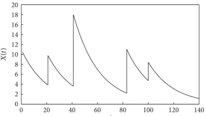
exponentially distributed with parameter 𝜇. With the above response function, the filtered Poisson process behaves as in

Figure 1. Actually, this behavior depends on the form of the response function, but not on the distribution of the time between the events. Therefore, the same behavior would be

observed in the case when {𝑁(𝑡), 𝑡 ≥ 0} is a renewal process. Remember that a Poisson process is a particular renewal process.

To model the daily flows of rivers given their most recent observed values, conceptual and physical models based on the filtered Poisson process have been widely used

successfully for many decades; see, for example, Weiss [1],

Kelman [2], Koch [3], and Konecny [4]. Filtered Poisson

processes are still being used to model various phenomena

in civil engineering; see Yin et al. [5] and Miyamoto et al. [6].

Now, especially in hydrological applications, the form of

the response function in (2) is taken for granted rather than

being justified by the observations of the variable of interest. Actually, it is generally simply an assumption made to obtain a mathematically tractable model.

Similarly, the actual distribution of the 𝑌𝑛’s is not

inves-tigated. However, if one is only interested in forecasting the value of 𝑋(𝑡+𝛿), based on the values of the process up to time 𝑡, this does not really cause a problem because the forecast is

normally based on the mean of the 𝑌𝑛’s, and the distribution

itself is not needed.

Finally, and even more importantly, the assumption that

{𝑁(𝑡), 𝑡 ≥ 0}is indeed a Poisson process is not tested. Again,

this is a simplifying assumption, because one can then make use of the nice properties of the Poisson process, notably the fact that it has independent and stationary increments.

Next, notice that, with the response function in (2), the

effect on the value of the process of an event that occurred at

Hindawi Publishing Corporation

International Journal of Engineering Mathematics Volume 2014, Article ID 593243, 9 pages http://dx.doi.org/10.1155/2014/593243

0 20 40 60 80 100 120 140 0 2 4 6 8 10 12 14 16 18 20 t X( t)

Figur e 1: Example of a trajectory of a filtered Poisson process definedby (1) and (2).

time 𝜏_𝑛 is maximum at that time instant and {𝑋(𝑡), 𝑡 ≥ 0}

has discontinuities at the arrival times of the events of the Poisson process. In the case of the application in hydrology that consists in modeling the flow of rivers, if one looks at real hydrographs, one sees that there is a more or less extended period of time during which the flow increases from a minimum to a maximum. Even if river flows data are generally available on a daily basis, one does not observe very sudden increases of the flow, followed by an exponential decrease. Rather, it takes on average two to three days for the flow to reach a maximum, and the decrease is more or less rapid.

To obtain a more realistic model for the variations of river flows, by taking into account the periods of flow increase,

Lefebvre and Guilbault [7] used the following response

function:

𝑤 (𝑡, 𝜏𝑛, 𝑌𝑛) = 𝑌𝑛(𝑡 − 𝜏𝑛)𝑑𝑒−(𝑡−𝜏𝑛)/𝑐, (3)

where 𝑑 is a positive parameter. With this response function,

the river flow begins to increase immediately after time 𝜏𝑛,

but the maximum is reached after 𝑑𝑐 time units (i.e., generally days) and then it starts to decrease. Their work was improved by the authors, who provided a method to estimate the parameter 𝑑. They found that, for the applications that they considered, 𝑑 was in the interval (0,1).

With a Poisson process being a continuous-time Markov chain, the time that the process spends in a given state is exponentially distributed, which is a strictly decreasing

density function. Let 𝑇₁, 𝑇₂, . . . be the times between two

successive events, that is, the interarrival times. In the case of river flows, the interarrival time is generally a random variable with a density function that is increasing at first. Hence, the assumption that {𝑁(𝑡), 𝑡 ≥ 0} is a Poisson process is at least doubtful.

In Lefebvre [8], the author tested the hypothesis that

the 𝑇𝑛’s are exponentially distributed. He found that, for the

Delaware River, it was not accurate. Instead, it was shown that both a gamma and a Rayleigh distribution fitted the data much better. The objective was to forecast the peak flows of the Delaware River, which is a difficult task due to the very weak correlation between the successive peaks. To try to forecast these peak flows, the author used a filtered renewal

process as a model for the river flow. An advantage in using a Rayleigh distribution for the interarrival time is that the filtered renewal process can be transformed into a filtered Poisson process by working on a different time scale.

Poisson and renewal processes have been used in hydrol-ogy to model low flows (see, for instance, Loaiciga and

Leipnik [9] and Yagouti et al. [10]) as well as various physical

phenomena such as traffic noise (see Marcus [11]). Andersen

[12, 13] gave new theoretical results on filtered renewal

processes (see also the references therein).

Theaim of the present paper is to show that we can obtain

more accurate short-term forecasts of river flows by making use of filtered renewal processes rather than filtered Poisson processes. To do so, we will first need to develop a formula to forecast the flow at time 𝑋(𝑡 + 𝛿), given the history of the process up to time 𝑡. Because we cannot appeal to the memoryless property of the exponential distribution, the task of finding an estimator for 𝑋(𝑡+𝛿) is more difficult. The values of the river flow before time 𝑡 must be taken into account, contrary to the case of filtered Poisson process, for which the forecasts depend only on 𝑋(𝑡).

Moreover, because we want to clearly see the improve-ment obtained by using a more realistic distribution for the interarrival time, we will take the response function

defined in (2). Indeed, as mentioned above, filtered Poisson

processes having this response function are commonly used in hydrology, and the forecasting formulas are then easy to derive and implement. Therefore, it will be easier to judge the quality of the model that we propose.

In the next section, filtered renewal processes will be formally defined and the formulas needed to forecast the river

flows will be developed. Then, inSection 3, the results will

be applied to forecast the flows of the Delaware and Hudson Rivers. Finally, a few concluding remarks will be made in

Section 4.

2. River Flows Modeled as a Filtered

Renewal Process

Let 𝑋(𝑡) denote the flow of a certain river at time 𝑡. We assume that

𝑋 (𝑡) =𝑁(𝑡)∑

𝑛=1

𝑌_𝑛𝑒−(𝑡−𝜏𝑛)/𝑐 (𝑋 (𝑡) = 0 if 𝑁 (𝑡) = 0) , (4)

in which {𝑁(𝑡), 𝑡 ≥ 0} is a renewal process. The 𝜏_𝑛’s are the

arrival times of the events of the process {𝑁(𝑡), 𝑡 ≥ 0}, and the

times 𝑇_𝑛 = 𝜏_𝑛−𝜏_𝑛−1between the successive renewals are

inde-pendent and identically distributed random variables. Finally,

the (positive) random variables 𝑌1, 𝑌2, . . . are independent

and identically distributed (and independent of {𝑁(𝑡), 𝑡 ≥ 0}).

Thus, the process is characterized by the sudden increases of the river flow caused by the events that occur at times

𝜏₁, 𝜏₂, . . .. A renewal cycle is defined as the time 𝑇𝑛between

two consecutive peaks. For the interarrival time, the following distributions (in addition to the exponential distribution) will

be considered inSection 3: lognormal, gamma, Weibull, and

International Journal of Engineering Mathematics 3 Next, in order to be able to forecast the river flow at time

𝑡 + 𝛿, we must first estimate the parameter 𝑐 that appears in the response function. If there are no signals between 𝑡 and 𝑡 + 1, then 𝑋(𝑡 + 1) is given by

𝑋 (𝑡 + 1) = 𝑒−1/𝑐𝑋 (𝑡) . (5)

Hence, to estimate the parameter 𝑐, we can consider all the days where the flow decreased in the data set and calculate the ratio 𝑋(𝑡+1)/𝑋(𝑡). The point estimate of 𝑐 is then derived from the arithmetic mean 𝑅 of this ratio:

̂𝑐 = − 1

ln 𝑅. (6)

In the case of the random variables 𝑌_𝑛, which constitute

a random sample of a parent random variable 𝑌, their exact distribution is not needed. Indeed, only the expected value of

𝑌will be used to forecast the value of 𝑋(𝑡 + 𝛿). Therefore, we

simply have to compute the mean increase of the river flow during the calibration period of the model.

We will now derive formulas to estimate the river flow one and two days in advance. These formulas can be used with any distribution for the interarrival time 𝑇, which denotes the parent variable of the 𝑇𝑛’s.

2.1. Forecasting the Flow at Time 𝑡 + 1. We will first try to

forecast the river flow at time 𝑡 + 1, given all the information available up to 𝑡. To do so, we assume that there will be at most one event in the interval (𝑡, 𝑡 + 1]. At any rate, as mentioned above, in practice flow values are generally available on a daily basis. Therefore, it is not really possible to determine whether more than one event occurred in (𝑡, 𝑡 + 1]. When it does happen, these events can be considered as a single large event. Apart from the case when the interarrival time 𝑇 has an exponential distribution, we must take the history of the process into account to calculate the probability that there will indeed be an event in (𝑡, 𝑡 + 1]. Let

𝑈_𝑖= 𝜏_{𝑁(𝑡)+𝑖}− 𝜏_{𝑁(𝑡)+𝑖−1} for 𝑖 = 1, 2, . . . . (7)

That is, 𝑈_𝑖is the time elapsed between the (𝑖 − 1)st and the 𝑖th

event after the most recent one that occurred before or at time

𝑡. The random variables 𝑇 and 𝑈₁are identically distributed.

We must compute

𝑝_𝑘:= 𝑃 [𝑈₁≤ 𝑘 + 1 | 𝑈₁> 𝑘] , (8)

where 𝑘 is the (integer) number of days since the most recent signal was observed. We have

𝑝_𝑘= ∫

𝑘+1

𝑘 𝑓𝑈1(𝑢) 𝑑𝑢

∫_𝑘∞𝑓𝑈1(𝑢) 𝑑𝑢

. (9)

With the help of a mathematical software, we can obtain numerical values of this probability for any density function

𝑓_𝑈1and any value of 𝑘.

Next, if 𝑇 is exponentially distributed, it is well known that, given that there is a signal (i.e., an event) between 𝑡 and

𝑡 + 1, the conditional density of 𝑇 is uniform on the interval (𝑡, 𝑡 + 1], so that the signal in question occurred on average at time 𝑡 + 1/2. In the general case, we must compute the

conditional density function of 𝑈1in the interval (𝑘, 𝑘 + 1],

given that 𝑈1> 𝑘.

If there is indeed a signal between 𝑡 and 𝑡 + 1, the forecast of the river flow at time 𝑡 + 1 would be

𝑍𝑘:= 𝑋 (𝑡) 𝑒−1/̂𝑐+ 𝐸 [𝑌]_{𝑃 [𝑈}1 1> 𝑘] × ∫𝑘+1 𝑘 𝑒 −(𝑘+1−𝑢)/̂𝑐_𝑓 𝑈1(𝑢) 𝑑𝑢. (10)

Therefore, the forecast of the river flow at time 𝑡+1, given the entire history of the process up to 𝑡, is given by

̂ 𝑋 (𝑡 + 1) = 𝑋 (𝑡) 𝑒−1/̂𝑐(1 − 𝑝𝑘) + 𝑍𝑘𝑝𝑘 = 𝑋 (𝑡) 𝑒−1/̂𝑐+ 𝑝_𝑘𝐸 [𝑌]_{𝑃 [𝑈}1 1> 𝑘] × 𝑒−(𝑘+1)/̂𝑐∫𝑘+1 𝑘 𝑒 𝑢/̂𝑐_𝑓 𝑈1(𝑢) 𝑑𝑢. (11)

2.2. Forecasting the Flow at Time 𝑡 + 2. Let 𝑈_1,𝑘 = 𝑈₁ |

{𝑈₁> 𝑘}. To forecast the river flow at time 𝑡 + 2, given all the

information available up to time 𝑡, we need the distribution

of the random variable 𝑆𝑘 := 𝑈1,𝑘+ 𝑈2, where 𝑈2is defined in

(7).

We now assume that the probability that there will be more than two signals in the interval (𝑡, 𝑡 + 2] is negligible

(irrespective of the value of 𝑘). The density function of 𝑆𝑘 is

given by the convolution of the density functions of 𝑈_1,𝑘and

𝑈₂:

𝑓_𝑆𝑘(𝑠 + 𝑘) = ∫∞

𝑘 𝑓𝑈1,𝑘(𝑢) 𝑓𝑈2(𝑠 + 𝑘 − 𝑢) 𝑑𝑢. (12)

Since 𝑈2is a nonnegative random variable, we can write that

𝑓𝑆𝑘(𝑠 + 𝑘) = ∫

𝑠+𝑘

𝑘 𝑓𝑈1,𝑘(𝑢) 𝑓𝑈2(𝑠 + 𝑘 − 𝑢) 𝑑𝑢 for 𝑠 > 0.

(13) In the case when 𝑇 has an exponential distribution with

parameter 𝜆, we know that (𝑆𝑘− 𝑘)has a gamma distribution

with parameters 𝛼 = 2 and 𝜆. In the other cases, we must generally evaluate the above integral numerically.

Thevalue of 𝑋(𝑡 + 2) is given by 𝑋 (𝑡 + 2) = { { { { { { { { { { { { { { { 𝑒−2/𝑐_{𝑋 (𝑡) if 𝑈} 1,𝑘> 𝑘 + 2, 𝑒−2/𝑐𝑋 (𝑡) + 𝑌1∗𝑒−(𝑘+2−𝑈1,𝑘)/𝑐 if 𝑈1,𝑘≤ 𝑘 + 2 and 𝑈2> 2 − (𝑈1,𝑘− 𝑘) , 𝑒−2/𝑐𝑋 (𝑡) + 𝑌1∗𝑒−(𝑘+2−𝑈1,𝑘)/𝑐 if 𝑈1,𝑘+ 𝑈2≤ 𝑘 + 2 +𝑌∗ 2𝑒−(2−𝑈2)/𝑐 (and 𝑈3> 2 − (𝑈1,𝑘− 𝑘) − 𝑈2) , (14) where 𝑌∗

𝑖 denotes the size of the 𝑖th signal in the interval (𝑡, 𝑡+

2]. As mentioned above, we assume that

𝑃 [𝑈₃> 2 − (𝑈_1,𝑘− 𝑘) − 𝑈₂] ≃ 1. (15)

We must first compute

𝑝_1,𝑘:= 𝑃 [𝑈_1,𝑘∈ (𝑘, 𝑘 + 2]] . (16)

When 𝑈1has an exponential distribution with parameter 𝜆,

𝑝1,𝑘= 𝑃 [𝑈1∈ (0, 2]] = 1 − 𝑒−2𝜆. (17) In general, we have 𝑝1,𝑘= ∫_𝑘𝑘+2𝑓𝑈1(𝑢) 𝑑𝑢 ∫_𝑘∞𝑓_𝑈1(𝑢) 𝑑𝑢. (18) Next, 𝑝_2,𝑘:= 𝑃 [𝑈_1,𝑘+ 𝑈₂∈ (𝑘, 𝑘 + 2]] ≡ 𝑃 [𝑆𝑘∈ (𝑘, 𝑘 + 2]] = ∫2 0 𝑓𝑆𝑘(𝑠 + 𝑘) 𝑑𝑠 = ∫2 0 [∫ 𝑠+𝑘 𝑘 𝑓𝑈1,𝑘(𝑢) 𝑓𝑈2(𝑠 + 𝑘 − 𝑢) 𝑑𝑢] 𝑑𝑠. (19)

Alternatively, using the fact that 𝑈_1,𝑘 and 𝑈₂ (≥ 0)are

independent random variables, we may write that 𝑝_2,𝑘:= 𝑃 [𝑈_1,𝑘+ 𝑈₂∈ (𝑘, 𝑘 + 2]] = ∫𝑘+2 𝑘 𝑃 [𝑈1,𝑘+ 𝑈2∈ (𝑘, 𝑘 + 2] | 𝑈1,𝑘= 𝑢 ] 𝑓𝑈1,𝑘(𝑢) 𝑑𝑢 = ∫𝑘+2 𝑘 𝑃 [𝑈2∈ (𝑘 − 𝑢 , 𝑘 + 2 − 𝑢 ]] 𝑓𝑈1,𝑘(𝑢) 𝑑𝑢 = ∫𝑘+2 𝑘 [∫ 𝑘+2−𝑢 0 𝑓𝑈2(V) 𝑑V] 𝑓𝑈1,𝑘(𝑢) 𝑑𝑢. (20) Finally, by independence, 𝑃 [{𝑈_1,𝑘≤ 𝑘 + 2} ∩ {𝑈₂> 2 − (𝑈_1,𝑘− 𝑘)}] = ∫𝑘+2 𝑘 𝑃 [𝑈2∈ (𝑘 + 2 − 𝑢 , ∞)] 𝑓𝑈1,𝑘(𝑢) 𝑑𝑢 = ∫𝑘+2 𝑘 [∫ ∞ 𝑘+2−𝑢𝑓𝑈2(V) 𝑑V] 𝑓𝑈1,𝑘(𝑢) 𝑑𝑢 = ∫𝑘+2 𝑘 [1 − ∫ 𝑘+2−𝑢 0 𝑓𝑈2(V) 𝑑V] 𝑓𝑈1,𝑘(𝑢) 𝑑𝑢 = 𝑝_1,𝑘− 𝑝_2,𝑘. (21)

Theforecast of the river flow at time 𝑡+2, given the entire

history of the process up to time 𝑡, is thus given by ̂ 𝑋 (𝑡 + 2) = 𝑋 (𝑡) 𝑒−2/̂𝑐(1 − 𝑝_1,𝑘) + {𝑋 (𝑡) 𝑒−2/̂𝑐+ 𝐸 [𝑌] ∫𝑘+2 𝑘 𝑒 −(𝑘+2−𝑢)/̂𝑐_𝑓 𝑈1,𝑘(𝑢) 𝑑𝑢} × (𝑝1,𝑘− 𝑝2,𝑘) + {𝑋 (𝑡) 𝑒−2/̂𝑐+ 𝐸 [𝑌] ∫𝑘+2 𝑘 𝑒 −(𝑘+2−𝑢)/̂𝑐_𝑓 𝑈1,𝑘(𝑢) 𝑑𝑢 + 𝐸 [𝑌] ∫𝑘+2 𝑘 [∫ 𝑘+2−𝑢 0 𝑒 −(2−V)/̂𝑐_𝑓 𝑈2(V) 𝑑V] × 𝑓_𝑈1,𝑘(𝑢) 𝑑𝑢} 𝑝2,𝑘 = 𝑋 (𝑡) 𝑒−2/̂𝑐+ {𝐸 [𝑌] ∫𝑘+2 𝑘 𝑒 −(𝑘+2−𝑢)/̂𝑐_𝑓 𝑈1,𝑘(𝑢) 𝑑𝑢} 𝑝1,𝑘 + {𝐸 [𝑌] ∫𝑘+2 𝑘 [∫ 𝑘+2−𝑢 0 𝑒 −(2−V)/̂𝑐_𝑓 𝑈2(V) 𝑑V] × 𝑓_𝑈1,𝑘(𝑢) 𝑑𝑢} 𝑝_2,𝑘

International Journal of Engineering Mathematics 5 = 𝑋 (𝑡) 𝑒−2/̂𝑐+ {𝐸 [𝑌] 𝑒−(𝑘+2)/̂𝑐∫𝑘+2 𝑘 𝑒 𝑢/̂𝑐_𝑓 𝑈1,𝑘(𝑢) 𝑑𝑢} 𝑝1,𝑘 + {𝐸 [𝑌] ∫𝑘+2 𝑘 [𝑒 −2/̂𝑐_∫𝑘+2−𝑢 0 𝑒 V/̂𝑐_𝑓 𝑈2(V) 𝑑V] × 𝑓𝑈1,𝑘(𝑢) 𝑑𝑢} 𝑝2,𝑘. (22)

3. Forecasting the Flows of the Delaware and

Hudson Rivers

To assess the quality of the forecasts obtained with the renewal filtered process, we need to apply the formulas developed in the previous section to real-life data. As in

[7], we chose the Delaware and Hudson Rivers, located

in the United States, at the Montague (01438500) and the North Creek (01315500) gage stations, respectively. The flow values are available on the Internet at the following address:

http://nwis.waterdata.usgs.gov. To calibrate the model, we used the data from October 2008 to September 2009.

Remarks. (i) When one is dealing with real-life data, things are

not as simple as the mathematical models suggest. Looking at the actual hydrograph of the Delaware River, we observe a number of weak peaks that occur while the flow is decreasing and for which the increasing period lasts only one day before the flow resumes its decline. Similarly, there are sometimes small increases of the flow value occurring just after a minimum was observed that last only one day. In building the data set, there is always a subjective part. We decided to neglect these weak peaks, thus considering only the peaks that appear quite clearly in the hydrograph.

(ii) Because the river flow is observed on a daily basis, we must discretize the set of possible values taken by the interarrival time 𝑇. We computed the number 𝑘 of days elapsed between consecutive peaks in the data set. In the case of the first observed peak, 𝑘 is the number of days elapsed since the beginning of the calibration period. Then, 𝑘 is obtained by subtracting the arrival times of the consecutive peaks. Notice that 𝑘 is greater than or equal to 1.

We first consider the Delaware River. For this river, we found that the average value 𝑇 of the interarrival times in the data set is equal to 6.8889 days. Moreover, the standard

deviation of the observations is given by 𝑠𝑇 = 3.8977days.

Based on these values, one may at once conclude that 𝑇 is very unlikely to be exponentially distributed. Indeed, remember that the mean and the standard deviation of an exponential distribution with parameter 𝜆 are both equal to 1/𝜆.

Next, the value of the point estimate of the (unitless)

parameter 𝑐 (see (6)) is ̂𝑐 = 9.2592, and the average value of

the magnitude 𝑌 of the signals is given by 𝑌 = 984.6121 cubic feet per second.

For the distribution of the random variable 𝑇, we tested the following models:

(i) an exponential distribution with parameter 𝜆,

0 0.05 0.1 0.15 0.2 0.25 0.3 0.35 0.4 0 0.1 0.2 0.3 0.4 0.5 0.6 0.7 0.8 0.91 T F( t) Empirical CDF Lognormal Exponential Gamma Weibull Rayleigh

Figure 2: Empirical and fitted distribution functions for the random variable 𝑇 (Delaware River).

0 0.2 0.4 0.6 0.8 1 1.2 1.4 0 0.1 0.2 0.3 0.4 0.5 0.6 0.7 0.8 0.91 Empirical CDF Lognormal Exponential Gamma Weibull Rayleigh T F( t)

Figure 3: Empirical and fitted distribution functions for the random variable 𝑇 (Hudson River).

(ii) a lognormal distribution with parameters 𝜇 and 𝜎, (iii) a gamma distribution with shape parameter 𝛼 and

scale parameter 𝜆,

(iv) a Weibull distribution with shape parameter 𝜆 and scale parameter 𝜅,

(v) a Rayleigh distribution with parameter 𝜎.

Table 1 summarizes the results of the chi-square goodness-of-fit tests for each distribution and gives the respective parameter estimates. We find that, as expected, the exponential distribution is rejected, whereas the other distributions are all accepted, according to the 𝑃-values of the tests. The empirical cumulative distribution function as well as the distribution functions of the various models

considered above is shown inFigure 2. We clearly see that

the exponential distribution does not fit the data nearly as well as the other four models.

Now, in the case of the filtered Poisson process (1) with the

Table 1: Goodness-of-fit tests for the distribution of the random variable 𝑇 (Delaware River).

Distribution Exponential Lognormal Gamma Weibull Rayleigh

Parameters 1/6.8889 1.7574, 0.6187 3.0544, 2.2554 7.7974, 1.8975 5.5817

𝑃-value 0.0344 0.7887 0.7723 0.6927 0.7008

Table 2: Criteria for comparing the forecasting models (Delaware River).

Filtered renewal process Filtered Poisson process Lognormal Gamma Weibull Rayleigh Exponential 𝑋(𝑡 + 1) Mape 12.58% 12.49% 12.55% 12.56% 12.76% Nash 0.8288 0.8290 0.8287 0.8287 0.8356 Pc 0.1674 0.1664 0.1663 0.1669 0.2522 Corr 0.9188 0.9186 0.9180 0.9188 0.9187 𝑋(𝑡 + 2) Mape 20.36% 20.33% 20.34% 20.34% 21.83% Nash 0.5447 0.5445 0.5445 0.5445 0.5573 Pc 0.2930 0.2893 0.2869 0.2863 0.3344 Corr 0.7735 0.7732 0.7731 0.7730 0.7734

time 𝑡 + 1 we compute the expected value of 𝑋(𝑡 + 1) given all the past observations. Because of the memoryless property of the exponential distribution, we find that this conditional expectation only depends on the most recent value of the flow,

that is, 𝑋(𝑡). We obtain (see [7]) that

𝐸 [𝑋 (𝑡 + 1) 𝑋] = (𝑡) 𝑒−1/𝑐𝑋 (𝑡) + 𝐸 [𝑋 (1)] , (23)

where

𝐸 [𝑋 (1)] = 𝜆𝑐_𝜇 (1 − 𝑒−1/𝑐) . (24)

Similarly, to estimate the river flow at time 𝑡 + 2, we only need to calculate 𝐸 [𝑋 (𝑡 + 2) | 𝑋 (𝑡)] = 𝐸 [ ∑ 𝑛:0≤𝜏𝑛≤𝑡+2 𝑌_𝑛𝑒−(𝑡+2−𝜏𝑛)/𝑐_{| 𝑋 (𝑡)]} = 𝑒−2/𝑐𝐸 [ ∑ 𝑛:0≤𝜏𝑛≤𝑡 𝑌_𝑛𝑒−(𝑡−𝜏𝑛)/𝑐| 𝑋 (𝑡)] + 𝐸 [ ∑ 𝑛:𝑡<𝜏𝑛≤𝑡+2 𝑌_𝑛𝑒−(𝑡+2−𝜏𝑛)/𝑐| 𝑋 (𝑡)] = 𝑒−2/𝑐𝑋 (𝑡) + 𝐸 [𝑋 (2)] , (25) where 𝐸 [𝑋 (2)] = 𝜆𝑐_𝜇 (1 − 𝑒−2/𝑐) . (26)

Moreover, we have that lim 𝑡 → ∞𝐸 [𝑋 (𝑡)] = 𝜆𝑐 𝜇, (27) lim 𝑡 → ∞Var [𝑋 (𝑡)] = 𝜆𝑐𝜇2, (28) lim 𝑡 → ∞𝜌𝑋(𝑡),𝑋(𝑡+𝛿)= 𝑒 −𝛿/𝑐_{, (29)}

where 𝜌_{𝑋(𝑡),𝑋(𝑡+𝛿)}denotes the correlation coefficient of 𝑋(𝑡)

and 𝑋(𝑡 + 𝛿).

By making use of these three equations, we can estimate the parameter 𝜆 of the Poisson process, the parameter 𝜇 of

the assumed exponential distribution of the 𝑌𝑛’s, and the

parameter 𝑐 in the response function. Actually, we do not need point estimates of 𝜆 and 𝜇 to forecast the flow. From

(27), we deduce that we can simply estimate the ratio 𝜆𝑐/𝜇

that appears in both (24) and (26) by the mean value of the

observed data when the process is in steady state. Finally, to estimate the parameter 𝑐, we first compute the empirical

correlation coefficient 𝑟1between the flow values at times 𝑡

and 𝑡 + 1 and then we set ̂𝑐 = −1/ ln(𝑟1) (see (29)). With

the value of 𝑟₁being close to 1, the previous formula is well

defined.

Remark. If one is only interested in forecasting the river flow

at time 𝑡 + 𝛿, one may estimate 𝑐 by computing the empirical

value of 𝜌_{𝑋(𝑡),𝑋(𝑡+𝛿)}and making use of (29).

We are now ready to compare the forecasts derived from both the filtered Poisson process and the filtered renewal process with the various distributions considered for the interarrival time 𝑇. We used the formulas given above to forecast the flow of the Delaware River for the 89-day period from February to April 2010.

To assess the accuracy of the forecasts, we consider four criteria commonly used in hydrology: the mean absolute

percentage error (Mape), the Nash criterion (Nash), the peak criterion (Pc), and the correlation coefficient (Corr) between

the observed and forecasted values.

The Nash criterion is based on the mean square error and is used to assess the predictive power of hydrological models. It evaluates the quality of the forecasts from the differences

International Journal of Engineering Mathematics 7

Table 3: Goodness-of-fit tests for the distribution of the random variable 𝑇 (Hudson River).

Distribution Exponential Lognormal Gamma Weibull Rayleigh

Parameters 1/8.3488 1.8754, 0.6625 9.2134, 1.3399 2.1785, 3.8324 7.9978

𝑃-value 0.0013 0.6983 0.3203 0.2532 0.000139

Table 4: Criteria for comparing the forecasting models (Hudson River).

Filtered renewal process Filtered Poisson process

Lognormal Gamma Weibull Exponential

𝑋(𝑡 + 1) Mape 12.33% 12.14% 12.33% 15.58% Nash 0.8240 0.8243 0.8240 0.8360 Pc 0.2875 0.2895 0.2872 0.4818 Corr 0.9146 0.9146 0.9146 0.9146 𝑋(𝑡 + 2) Mape 20.84% 21.00% 21.15% 32.78% Nash 0.5841 0.5838 0.5835 0.6222 Pc 0.4558 0.4533 0.4518 0.5575 Corr 0.7908 0.7909 0.7910 0.7910 ×104 0 10 20 30 40 50 60 70 80 90 0 0.5 1 1.5 2 2.5 3 3.5 4 Days Ri ver flo w Observed value Predicted value (FPP) Predicted value (FRP)

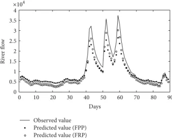
Figur e 4: Observed and forecasted values of the flow of the Delaware River at time 𝑡 + 1.

between the expected and observed daily values. It is equal to 1in case of a perfect fit. For its part, the peak criterion is used to measure the quality of the forecasts during the critical peak period. The closer to 0 it is, the better the forecasts are.

Table 2displays the results obtained with the two compet-ing models. Lookcompet-ing at these results, we notice that the Mape, Nash, and Corr criteria yield practically the same values for the filtered renewal and filtered Poisson processes. However, the filtered renewal process did much better than the filtered Poisson process when we consider the peak criterion. This criterion is especially important because accurate forecasts are really needed during the peak period.

We now turn to the Hudson River. The value of the point estimate of the constant 𝑐 for this river is ̂𝑐 = 9.1172 and the average magnitude of the signals is 𝑌 = 229.2533, which is much smaller than in the case of the Delaware River.

Proceeding as above, we performed chi-square goodness-of-fit tests for the various distributions considered. The results

×104 0 10 20 30 40 50 60 70 80 90 0 0.5 1 1.5 2 2.5 3 3.5 4 Days Ri ver flo w Observed value Predicted value (FPP) Predicted value (FRP)

Figur e 5: Observed and forecasted values of the flow of the Delaware River at time 𝑡 + 2.

are presented inTable 3(see alsoFigure 3). This time, we see

that both the exponential and Rayleigh distributions must be rejected, while the lognormal distribution clearly provides the best fit to the data.

The values of the four criteria used to compare the models

are shown inTable 4. We discarded the Rayleigh distribution,

because it yielded a very bad fit to the data. As in the case of the Delaware River, the values of the Nash and Corr criteria are quite similar, while the important peak criterion and the Mape criterion are much smaller for the filtered renewal process than for the filtered Poisson process.

Finally, we present the observed and forecasted values of the flows of the Delaware and Hudson Rivers at times 𝑡 + 1

and 𝑡+2 in Figures4,5,6, and7, based on the filtered Poisson

process (FPP) and the filtered renewal process (FRP) with a lognormal distribution for the interarrival time 𝑇. Notice that the filtered renewal process is generally better than the filtered

0 2000 4000 6000 8000 10000 12000 Ri ver flo w 0 10 20 30 40 50 60 70 80 90 Days Observed value Predicted value (FPP) Predicted value (FRP)

Figure 6: Observed and forecasted values of the flow of the Hudson River at time 𝑡 + 1. 0 2000 4000 6000 8000 10000 12000 Ri ver flo w 0 10 20 30 40 50 60 70 80 90 Days Observed value Predicted value (FPP) Predicted value (FRP)

Figur e 7: Observed and forecasted values of the flow of the Hudson River at time 𝑡 + 2.

Poisson process at forecasting high flow values, which is our main concern.

4. Conclusion

In this paper, we were able to significantly improve the short-term hydrological forecasts produced by filtered Poisson processes by using a more realistic distribution for the inter-arrival time of the signals, thus working with filtered renewal processes. As we saw in the previous section, the filtered Poisson process, despite its lack of realism, is able to yield reasonable short-term forecasts. One possible explanation is the fact that the forecasting formulas derived from this model are very easy to implement. Also, contrary to the filtered renewal process, it does not require subjective decisions to estimate its various parameters. However, the filtered Poisson process was not able to produce forecasts as accurate as those derived from the filtered renewal process during the important peak period.

In addition to being used to forecast flow values, the models considered in this paper can also give us an estimate of the probability that the river flow will exceed a certain threshold in the next few days. This threshold may be a value that corresponds to a flow above which the risk of flooding is very high.

Finally, we could use the response function in (3) to

further improve the forecasts. To do so, we would have to be able to estimate the parameter 𝑑 in that response function and

then obtain formulas that generalize the ones in (11) and (22),

which is probably not an easy task.

Conflict of Interests

The authors declare that there is no conflict of interests regarding the publication of this paper.

Acknowledgment

Theauthors want to thank the anonymous reviewers for the

constructive comments.

References

[1] G. Weiss, “Shot noise models for the generation of synthetic streamflow data,” Water Resources Research, vol. 13, no. 1, pp. 101–108, 1977.

[2] J. Kelman, “A stochastic model for daily streamflow,” Journal of

Hydrology, vol. 47, no. 3-4, pp. 235–249, 1980.

[3] R. W. Koch, “A stochastic streamflow model based on physical principles,” Water Resources Research, vol. 21, no. 4, pp. 545–553, 1985.

[4] F. Konecny, “On the shot-noise streamflow model and its applications,” Stochastic Hydrology and Hydraulics, vol. 6, no. 4, pp. 289–303, 1992.

[5] Y.-J. Yin, Y. Li, and W. M. Bulleit, “Stochastic modeling of snow loads using a filtered Poisson process,” Journal of Cold Regions

Engineering, vol. 25, no. 1, pp. 16–36, 2010.

[6] H. Miyamoto, J. Morioka, K. Kanda et al., “A stochastic model for tree vegetation dynamics in river courses with interaction by discharge fluctuation impacts,” Journal of Japan Society of Civil

Engineers B1: Hydraulic Engineering, vol. 67, no. 4, pp. 1405–1410,

2012.

[7] M. Lefebvre and J.-L. Guilbault, “Using filtered Poisson pro-cesses to model a river flow,” Applied Mathematical Modelling, vol. 32, no. 12, pp. 2792–2805, 2008.

[8] M. Lefebvre, “A filtered renewal process as a model for a river flow,” Mathematical Problems in Engineering, vol. 2005, no. 1, pp. 49–59, 2005.

[9] H. A. Loaiciga and R. B. Leipnik, “Stochastic renewal model of low-flow streamflow sequences,” Stochastic Hydrology and

Hydraulics, vol. 10, no. 1, pp. 65–85, 1996.

[10] A. Yagouti, I. Abi-Zeid, T. B. M. J. Ouarda, and B. Bob´ee, “Revue de processus ponctuels et synth`ese de tests statistiques pour le choix d’un type de processus,” Journal of Water Science, vol. 14, no. 3, pp. 323–361, 2001.

[11] A. H. Marcus, “Traffic noise as a filtered Markov renewal process,” Journal of Applied Probability, vol. 10, no. 2, pp. 377– 386, 1973.

International Journal of Engineering Mathematics 9

[12] P. K. Andersen, “Filtered renewal processes with a two-sided impact function,” Journal of Applied Probability, vol. 16, no. 4, pp. 813–821, 1979.

[13] P. K. Andersen, “A note on filtered Markov renewal processes,”

Submit your manuscripts at

http://www.hindawi.com

Hindawi Publishing Corporation

http://www.hindawi.com Volume 2014

Mathematics

Hindawi Publishing Corporation

http://www.hindawi.com Volume 2014 Mathematical Problems in Engineering

Hindawi Publishing Corporation http://www.hindawi.com

Differential Equations International Journal of

Volume 2014

Hindawi Publishing Corporation

http://www.hindawi.com Volume 2014

Mathematical PhysicsAdvances in

Complex Analysis

http://www.hindawi.com Volume 2014

Optimization

Hindawi Publishing Corporation

http://www.hindawi.com Volume 2014

Combinatorics

Hindawi Publishing Corporation

http://www.hindawi.com Volume 2014

International Journal of

Journal of

Hindawi Publishing Corporation

http://www.hindawi.com Volume 2014

Function Spaces

Abstract and Applied Analysis Hindawi Publishing Corporation

http://www.hindawi.com Volume 2014 International Journal of Mathematics and Mathematical Sciences

Hindawi Publishing Corporation http://www.hindawi.com Volume 2014

The Scientific

World Journal

http://www.hindawi.com Volume 2014

Discrete Dynamics in Nature and Society

Hindawi Publishing Corporation

http://www.hindawi.com Volume 2014

Discrete Mathematics

Hindawi Publishing Corporation

http://www.hindawi.com Volume 2014 Hindawi Publishing Corporationhttp://www.hindawi.com Volume 2014

Stochastic Analysis