HAL Id: hal-01313233
https://hal.archives-ouvertes.fr/hal-01313233
Submitted on 13 Jan 2017HAL is a multi-disciplinary open access
archive for the deposit and dissemination of sci-entific research documents, whether they are pub-lished or not. The documents may come from teaching and research institutions in France or abroad, or from public or private research centers.
L’archive ouverte pluridisciplinaire HAL, est destinée au dépôt et à la diffusion de documents scientifiques de niveau recherche, publiés ou non, émanant des établissements d’enseignement et de recherche français ou étrangers, des laboratoires publics ou privés.
Robust dynamic schedule coordination control in the
supply chain
Dmitry Ivanov, Alexandre Dolgui, Boris Sokolov
To cite this version:
Dmitry Ivanov, Alexandre Dolgui, Boris Sokolov. Robust dynamic schedule coordination con-trol in the supply chain. Computers & Industrial Engineering, Elsevier, 2016, 94 (18–31), �10.1016/j.cie.2016.01.009�. �hal-01313233�
Computers & Industrial Engineering
Volume 94, April 2016, Pages 18–31
This is initial draft version, if any problem, please see the published article where the text is of better quality
Robust dynamic schedule coordination control in the supply chain
Dmitry Ivanov1*, Alexandre Dolgui2,Boris Sokolov3,4
1*
Berlin School of Economics and Law
Department of Business Administration; Chair of International Supply Chain Management 10825 Berlin, Germany
Phone: +49 30 85789155 E-Mail: [email protected] 2
Ecole Nationale Supérieure des Mines de Nantes IRCCYN, UMR CNRS 6597
La Chantrerie
4, rue Alfred Kastler - B.P. 20722 F-44307 NANTES Cedex 3, France
E-mail : [email protected], [email protected] 3
Saint Petersburg Institute for Informatics and Automation of the RAS (SPIIRAS) V.O. 14 line, 39 199178 St. Petersburg, Russia
E-Mail: [email protected] 4
ITMO University, St. Petersburg, Russia E-Mail: [email protected]
* Corresponding author Dmitry Ivanov
Abstract
Coordination plays crucial role in supply chain scheduling. In this paper, we extend the existing body of litera-ture on supply chain scheduling by representing the robust schedule coordination approach. A hybrid dis-crete/continuous flow shop supply chain with job shop processes at each supplier stage is studied with dynam-ic optimal control models. We consider operations, channel, resource and flow control models with multiple objectives. Computational procedure and model integration are described. Based on this model, we introduce a robust analysis of schedule coordination in the presence of disruptions in capacities and supply. The applica-tion of attainable sets opens a possibility to analyse feasible schedule execuapplica-tions under disrupapplica-tions. Subse-quently, we integrate the schedule coordination issues into robustness analysis, exemplify the developed ap-proach for the case of two-stage supply chain coordination, and derive managerial insights for both considered scheduling problem and application of dynamic control methods to supply chain schedule coordination in general.
Keywords: supply chain, control, coordination, scheduling, flow shop, robustness, attainable sets
Introduction
Continuous flow scheduling problems have their place in many industries such as gas, oil, chemicals, glass and fluids production as well as production of granular goods and steel details (Shah 2004, Puigjaner and Lainez 2008, Subramanian et al. 2013, Ivanov et al. 2013, Ivanov et al. 2015). Supply chains (SC) in the con-tinuous industry comprise multi-stage network of suppliers. Integration and coordination are two central is-sues in supply chain management (SCM) for such industries. In general, coordinated decision-making distin-guish SC scheduling problem as a specific research topic (Hall and Potts 2003, Chen 2010, Sawik 2009, Sawik 2013).
Details of mathematical models across the publications on SC scheduling differ, but most share a basic set of attributes: a finite sets of jobs, customers, and suppliers, fixed time span over which a schedule should be gen-erated, and multi-stage schedule coordination. Most recently, Sawik (2015) points out that although the im-pacts of schedule coordination on SC performance may be substantial, the research on coordinated scheduling optimization is fairly recent and there is still a research gap in regard to the magnitude of these impacts (Agnetis et al. 2006).
In addition, in recent years, disruptions in SC capacities occurred in greater frequency and intensity. These events rippled quickly through global SCs and caused significant losses in revenues. In this setting, the issues of the SC robustness become more and more important (Xu et al. 2014, Kim et al. 2015). When handing these issues, new challenges for SC scheduling exist that concern uncertainty and disruptions along with coordina-tion activities (Sawik 2013).
In this study, we focus on robust coordinated SC scheduling for the production systems with continuous mate-rial flows. Since the SC process typically has a multi-stage structure, the issue of capacity and supply disrup-tions is crucial for the overall SC schedule performance. The disrupdisrup-tions in processing and transportation ca-pacities may result in increase in flow times, makespan, tardiness, and decrease in throughput, on-time deliv-ery, and SC service level. In this setting, the dynamic schedule representation and schedule robustness analy-sis become important issues. Moreover, the coordination needs to be included in the scheduling and robust-ness analysis.
To the best of our knowledge, there is no published research on coordinated SC scheduling for the production systems with continuous flows and disruptions as well as schedule coordination considerations. The objective of this study is to extend the existing body of knowledge on SC scheduling by representing the robust sched-ule coordination in the hybrid continuous flow shop SC with job shop processes at each supplier in the dy-namic optimal control model.
State-of-the-art
In SCs, after the processing at the production plants (i.e., the suppliers), finished products can be delivered to the next production stage in the SC or to the customers. In terms of scheduling theory, we have a flow shop process (Johnson 1954, Gonzalez and Sahni 1978, Gupta et al. 2001). At the same time, at each stage in this
multistage environment, alternative executors (e.g., production plants and transportation modes) exist which
are unequal regarding different processing intensities. Once a job is assigned to a supplier, the processing of operations of this job can be done either in job- or flow- shop mode. Thus, the SC is a hybrid flow shop (Ribas et al. 2010). This creates flexibility in the process plan and requires both machine assignment and sequencing tasks (Patel et al. 2011).
The next characteristic of this SC is the integration of the production scheduling and transportation routing components which happens to be one of the most important problems in SCs (Sarker et al. 2009). Chen (2010) recommends considering such a problem as an integrated production and outbound distribution scheduling problem. A peculiarity of such a simultaneous consideration is that both machine structures and flow parame-ters may be uncertain and change in dynamics and are, therefore, non-stationary. In the context of SCs and taking into account standard scheduling methods, uncertainty in SC schedule parameters is accepted by re-search community as important and timely rere-search topic (Hall and Potts 2003, Agnetis et al. 2006).
The study by Hall and Potts (2003) considered benefits and challenges of coordinated decision-making within SC scheduling. Chen and Hall (2007) studied the conflicts and coordination in assembly systems where there are several suppliers providing components. Sarker and Diponegoro (2009) considered optimal production plans and shipment schedules in an SC with multiple suppliers, one manufacturer and multiple buyers subject to known demands of buyers. The overview by Chen (2010) identified that in integrated scheduling and logis-tics problems, it is necessary to define completion, departure, and delivery times for each job subject to time-based, cost-based or revenue-based indicators. Hall and Liu (2011) investigated the capacity allocation by a manufacturer subject to orders from distribution centers. Ullrich (2013) integrates production and outbound distribution scheduling in order to minimize total tardiness. Choi et al. (2013) study a SC scheduling and co-ordination problem where the manufacturer is a decision maker that selects the orders and aims to maximise its own profit.
In scheduling theory, considerable achievements can be stated regarding assignment and sequencing problems in the context of multi-stage systems (Blazewicz et al. 2001, Lauff & Werner, 2004, Aytug et al. 2005). Scheduling with alternative parallel machines has also been a large research avenue over the past few dec-ades. In such systems, the decision is to optimize both the selection of machines for each part and loading sequences of parts to machines to improve productivity. The review of Blazewicz et al. (1991) shows that especially for non-preemptive scheduling and even with identical machines, these problems are NP-hard. Most papers on multi-stage systems deal with problems, where the computational complexity represents the most critical challenge (Chiou et al., 2012). Another challenge is the different processing speed at the ma-chines which influence the task times (Kyparisis & Koulamas, 2006). Examples for multi-stage flow-shop scheduling problem with alternative machines at each stage with different time-dependent processing speed, and time-dependent machine availability can be found in the studies by Kyparisis & Koulamas (2006). Bożek and Wysocki (2015) analysed continuous flow flexible job shop (CF-FJS) problem that combines the flexible job shop (FJS) problem and a dedicated continuous material flow model. In this study, the operations are rep-resented by material flow functions derived by integration of arbitrarily defined speed patterns. A variable speed of processing and a continuous material flow lead to position-dependent processing times and overlap-ping in operations. A tabu search scheduling algorithm is proposed to solve the problem.
In the literature, the studies on schedule robustness aim at closing the gap between theory and practice regard-ing the uncertain nature of real environments for the schedule execution. A schedule that is able to achieve the planned performance in spite of disruptions is called robust (Sotskov et al. 2013, Sotskov and Werner 2013). Robustness analysis or robust optimization approaches for related problems in assembly line design and scheduling have been considered, for example, in the studies by (Sotskov et al., 2006, Dolgui and Kovalev, 2012a, Dolgui and Kovalev, 2012b, Hazir and Dolgui, 2013, Gurevsky et al., 2012, Gurevsky et al., 2013, Hazir and Dolgui, 2015). The method developed in this paper is complementary to the robust discrete optimi-zation.
In the analysis of schedule robustness, a number of particular features should be taken into account. In prac-tice, decision makers may want to judge on the trade-off between robustness and such performance measures
as makespan, flow time, or tardiness (Sotskov et al. 2013). Different approaches have been proposed so far since robustness is really a multi-faceted issue in operational research (Roy 2010). Artigues et al. (2005) pro-pose to generate a family of schedules instead of a unique one to maintain schedule robustness in a job shop environment. In the stochastic domain, probability density functions of the model parameters or perturbations are used in order to construct a robust schedule. For example, in the study by Al-Fawzan and Haouari (2005), schedule robustness is defined as the sum of the free slacks of the activities. The interval data domain has been addressed first in the study by Daniels and Kouvelis (1995) subject to processing time variability in a single machine environment with the objective of minimizing total flow time. The aim is to find a schedule whose performance degradation in its worst-case scenario is the least among all feasible schedules (i.e., the minimax regret).
Even though previous studies included a robustness objective into scheduling, they rarely considered multi-stage cases, alternative parallel machines, and flow shops where robustness and coordination are considered for continuous flows cases. Robustness in continuous time domain has not been explored in the scheduling settings so far although it has been extensively investigated in system dynamics and control theory (Mayne et al. 2000, Ivanov et al. 2012, Ivanov and Sokolov 2013). Recent application of control theory (CT) and optimal program control (OPC) to scheduling have been multi-facet. The studies by Holt et al. (1960), Hwang et al. (1967), Zimin and Ivanilov (1971) and Moiseev (1974) were among the first to apply the OPC and the maxi-mum principle to multi-level and multi-period master production scheduling that determined the production as an optimal control with a corresponding trajectory of the state variables (i.e., the inventory). This stream was continued by Kimemia and Gershwin (1983), who applied a hierarchical method in designing a solution pro-cedure, and by Khmelnitsky et al. (1997) for planning continuous-time flows in flexible manufacturing. The managers are always interested in non-deterministic approaches to scheduling where scheduling is inter-connected to the control function (MacCarthy, & Liu, 1993). The studies by Sarimveis et al. (2008) and Har-junkoski et al. (2014) showed a wide range of advantages regarding the application of CT models in combina-tion with other techniques to produccombina-tion and logistics. They include, first of all, a non-stacombina-tionary process view and accuracy of continuous time (Chen et al. 2012, Jula and Kones 2013). In addition, a wide range of analy-sis tools from CT regarding stability, controllability, adaptability, etc. may be used if a schedule is described in terms of control. Ivanov and Sokolov (2013) developed a CT framework for analysis of SC robustness, resilience, and stability. Wang et al. (2013) proposed a distributed scheduling algorithm called a closed-loop feedback simulation approach that includes adaptive control of the auction-based bidding sequence to prevent the first bid first serve rule and may dynamically allocate production resources to operations. Ivanov et al. (2015) apply OPC to distributed SC scheduling in the context of smart factory Industry 4.0.
However, the calculation of the OPC with direct methods of the continuous maximum principle has not been proved to be efficient (Ivanov and Sokolov 2012). The application of OPC to scheduling is not a trivial prob-lem for two reasons. First, a conceptual probprob-lem consists of the continuous values of the control variables. In scheduling, the decisions on start and completion time of operations are discrete. Second, a computational problem for applications of a direct method of the maximum principle exists. The optimality of schedule is in this setting a critical issue. These shortcomings set limitations on the application of OPC to purely combinato-rial problems. That is why the approach of this study combines continuous and discrete optimization.
3. Methodology and problem statement
3.1 Basic methodical principles of the proposed approach
The first main idea of the approach proposed is to use fundamental results gained in the OPC theory for the SC scheduling domain to describe the operations execution process (i.e., the time-dependent increase in the
processed operation volume) between the start and the completion time. In the approach proposed, the consid-eration of dynamic control models within the OPC axiomatic and on the basis of combining mathematical programming (MP) and OPC. A peculiarity of OPC models are constraints (economic, technological, coopera-tion, etc.) on the control, state variables, and their combinations. A particular feature of the proposed approach is that the process control models will be presented as a stationary dynamic linear system while the non-linearity will be transferred to the model constraints. This allows us to ensure convexity and to use interval constraints. As such, a constructive possibility of discrete problem solving in a continuous manner occurs. In the scheduling model, a multi-step procedure for coordinated SC scheduling is implemented. At each in-stant of time while calculating solutions in the dynamic model with the help of the maximum principle, the linear programming (LP) problems to allocate jobs to resources and integer programming (IP) problems for (re)distributing material and time resources are solved with conventional capacitated LP/IP algorithms. The basic computational idea of this approach is the fact that the operation executions and machine availabilities are dynamically distributed in time over the planning horizon. As such, not all operations and machines are involved in the decision making at the same time. Therefore, it becomes quite natural to transit from large-size allocation matrices with a high number of binary variables to a scheduling problem that is dynamically de-composed (Ivanov et al. 2015). Following an approach to decompose the solution space and to use exact methods over its restricted sub-spaces, we propose to use the OPC theory for the dynamic decomposition of the scheduling problem. Indeed, OPC is mainly used for the dynamic decomposition but not for the calcula-tions. The computational procedure is transferred to the MP methods (Ivanov et al. 2013, Ivanov et al. 2015). The solution at each time point is calculated with MP. OPC is used for modeling the execution of the opera-tions and interlinking the MP soluopera-tions over the planning horizon. Hence, the solution procedure becomes independent of the continuous optimization algorithms and can be of discrete nature, e.g., an integer assign-ment model.
For solving the boundary problem, Pontryagin’s maximum principle is applied (Pontryagin et al. 1964). The maximum principle permits a decoupling of the considered dynamic problem over time using what are known as adjoint variables or shadow prices. The dynamic problem is decomposed into a series of static problems each of which holds at a single instant of time. The maximum principle guarantees that the optimal solutions of the instantaneous problems give an optimal solution to the overall problem (Pontryagin et al. 1964; Boltyanskiy, 1973; Sethi & Thompson, 2000). This property of OPC is very helpful when interconnecting MP and OPC elements.
3.2 Problem description
Fig. 1. Structural elements of the global scheduling model
“Job” comprises a set of operations to be completed at a supplier level according to some criteria such as de-livery date and ordered quantity.
“Operation“ is an action needed to complete a production process. Each operation is characterized by some parameters such as lead-time, processed quantity, resource consumption and material flow.
“Supplier” is a processing plant in the SC.
“Channel” is a unit needed for processing or delivering the products; in manufacturing, a channel can be a machine, a cell, or a processing center; in logistics, a channel can be, e.g., a road.
“Resource” is a unit needed for processing an operation in a channel; it can be a material, a technical device or a truck.
“Flow” is material flow characterizing by real and planned quantities, processing/transportation intensities and speed of flow volume change.
Jobs are executed in a flow-shop mode, i.e., there is a steady sequence of processing stages each of which contains some alternative suppliers. Once a job is assigned to a supplier, the operations of this job are execut-ed either in flow or job shop mode at some alternative channels. For transportation, different alternative chan-nels are available.
In addition, the considered problem captures the following features:
Processing speed of each machine is described as a function of time and is modelled by material flow functions (integrals of processing speed functions) and resulting processing time is, in general, chan-nel dependent
Processing, transportation, and warehouse capacities are included Setups are included in the analysis
Lot-sizes and release dates are known
Temporary capacity unavailability is included both in planned and perturbed modes Capacity degradation/recovery is considered
Impact of disturbances and coordination on performance with recovery consideration is included in the analysis with the help of the theory of attainable sets
Material supply dynamics is described in the resource control model The following performance indicators (objective functions) are considered:
Throughput Lead-time Makespan Waiting time
The first task is to find a coordinated schedule in the SC, i.e., to assign the jobs at each stage to alternative suppliers and determine start and completion times for each operation at the machines at each supplier. This will be done in Section 4. The second task consists of analyzing the impact of disruptions in capacities and supply on the attainability of the planned schedule performance. Subsequently, in Section 5 we integrate a schedule robustness analysis and exemplify the developed approach for the case of a two-stage supply chain coordination with the help of attainable sets.
Total lateness Time-to-recovery
Equal utilization of channels in the SC
4. Mathematical model
4.1 Notations
Consider the following sets:
- set of jobs A = {A, N} that are composed of a set of operations
- D
D(c){Dæ(i)}{Dæ(i,j)},i,jM,æKi(о),æK(о)i,j
;- set of suppliers B = {Bi, i M} and set of channels at each supplier C{C(i),ki,iM}; - set of resources in the SC
{S(i)}{N(i)},iM,Ki(r,1),Ki(r,2)
,
() (r,1)
) ( , i i i S K S is a set of storable resources at В(i) and N(i)
N(i),Ki(r,2)
is a set of non-storable resources at В(i);- set of manufacturing operations that can be fulfilled at supplier В(i)D(i)
Dæ(i),æKi(о)
;- set of logistics operations D(i,j)
Dæ(i,j),æK(о)i,j
subject to transportation between В(i) and В(j); - set of material flowsP
{P(æi),}{P(æ,i,j)},iM,æKi(о),æK(о)i,j,Ki(f)
;- set of material flows for ρ-types of materialsP(i)
{P(iæ),},iM,æKi(о),Ki(f)
subject toВ(i);
- set of material flows for ρ-types of materials P(i,j)
P(æ,i,j),i,jM,Ki(f)
subject to В(i) andВ(j).
- sets Г1, Г2 of precedence relations for different jobs and set iæ1,iæ2of precedence relations for op-erations Dæ(i,j)and Dæ(i).
Indices (o), (k), (r) and (f) inKi(о), Ki(r) andKi(f)describe the relations of the sets to operations (o), channels (k), machines (r), and material flows (f).
Assume that manufacturing and transportation capacities may be disrupted and:
- a supplier availability can be described by a given preset matrix time function i j (t) of time-spatial con-straints; we have i j (t)=1, if the delivery capacity between Bi and Bj is available and i j (t)=0, otherwise; - a channel availability can be described by the function iæj(t) (or æj(t)) that is equal to 1, if there are
available channels and for Bi and Bj at time t T for processing and equals 0, otherwise; - manufacturing and logistics capacity degradation/recovery dynamics can be described by a continuous
function ξij(t); ξij(t)=1 if the channel between Bi and Bj is 100% available and ξij(t)=0 if the channel is dis-rupted fully. All other values for ξij(t) in the interval [0;1] are possible.
4.2 Dynamic model for the operation control processes (model Mo)
The formal statement of the scheduling problem is produced as a dynamic interpretation of the operations execution processes.
Process model of operations execution:
) (i C C( j) (, ) æ j i D
) 3 , 0 ( ) 3 , 0 ( 1 1 ) , 2 , 0 ( æ æ ) , 2 , 0 ( æ 1 ) 1 , 0 ( ) 1 , 0 ( ; ) ( ) ( ; j j m j l j i j i ij i m j j x t t u x u u x j
(1) =1,...,n; j =1,...,m; i =1,...,m; æ =1,...,si Constraints: (2) (3) (4) (5)Start and end conditions:
(6) Objective functions:
n m j f o j T u J 1 1 ) 3 , ( ) o ( 1 ( ) (7)
m i m j f o j f o i T x T x J 1 1 ) 3 , ( ) 3 , ( ) o ( , , 2 ( ) ( ) (8)
1 ) 1 , ( ) o ( 3(
)
j f o nj fx
T
T
J
(9) (10)
æ , , T ) , 2 , 0 ( æ o) ( , 5 0 ) ( ) ( ) ( j T j i ij ij i f d u J (11)
m i s f o i o i i T x a J 1æ 1 2 ) , 2 , ( æ ) , 2 , ( æ ) o ( 6 ( ) (12)
n m i s m j l T T j i i i j f d u J 1 1æ 1 1 1 ) , 2 , 0 ( æ ) ( æ ) o ( 7 0 ) ( ) ( ~ ~ (13) Parameters:
( )
( )
0 2 1 ) 1 , 0 ( ) 1 , 0 ( ) 1 , 0 ( ) 1 , 0 ( 1 ) 1 , 0 (
t x a t x a u m j j
( )
()
0 2 æ 1 æ ~ ) , 2 , 0 ( ~ ) , 2 , 0 ( ~ ~ ) , 2 , 0 ( ~ ) , 2 , 0 ( ~ 1 ) , 2 , 0 ( æ
i i j t x a t x a u i i i i l j i } 1 , 0 { ) ( ; , 1 ) ( ; , 1 ) ( (0,1) 1 ) 1 , 0 ( 1 ) 1 , 0 (
u t j u t j uj t m j j u j
0,
; () {0,1};
()
0 ) ( (0,1) (0,3) (0,3) (0,2, ) (0,2, ) ) , 2 , 0 ( æ t u u t u a x t u j i js js j j j j i
x
O h
x
O h0(o) (o)(T0) ; 1(o) (o)(Tf)
æ , , , T ) , 2 , 0 ( æ æ o) ( , , 4 0)
(
)
(
)
(
j T j i j i ij i fd
u
J
) , 2 , ( ~ ) , 2 , ( ~ ) 1 , ( ) 1 , ( , , , io io o o a a a a , is(o,2,) i
a , ai(æo,1,) are planned manufacturing/transportation quantities for each operation (i.e., the end conditions); these values have to be reached in x(o,1)(t),x(o,1)(t),x(~,2, )(t),x(~o,2, )(t)
i o i , ) ( ) , 2 , ( t xiso i , ) ( ) , 1 , ( æ t xio at time t = Tf ; o) ( 1 o) ( 0 , h
h are known differential functions for setting the start and end conditions subject to state variables
х(о) = x1(o,1),...,xn(o,1),x11(o,2),...,xms(o,2),x11(o,3),...,xnm(o,3) т m at t = T0 and t = Tf. Decision variables: ) ( ) 1 , 0 ( t
x is a state variable characterizing the flow time for job A at each moment t
) ( ) , 2 , 0 ( æ t
xi is a state variable characterizing the flow time of the operationsDæ(i) or Dæ(i,j) ) ( ) 3 , 0 ( t
x is a state variable characterizing the gap between the planned completion time for all jobs and the actual completion time of the job A
) ( ) 1 , 0 ( t
uj ,ui(æ0j,2,)(t), are control variables; u(0j,1)(t)=1, if we have a transportation of a job A to Bj, ) ( ) 1 , 0 ( t
uj =0, otherwise; ui(æ0j,2,)(t)=1, if operation Dæ(i) or Dæ(i,j) is assigned to a λ-channel, ui(æ0j,2,)(t)=0, oth-erwise; u(0j,3)(t)=1 if Ais completed at time moment t and until Tf , u(0j,3)(t)=0, otherwise
Eq. (1) describes the process dynamics of operations execution for jobs Asee Figs 2-3).
m j j u x 1 ) 1 , 0 ( ) 1 , 0 ( means that at each point of time where if u(0j,1)(t)=1, the operation is being processed and its
processed quantity increases.
m j j i ij i t u x 1 ) , 2 , 0 ( æ ) , 2 , 0 ( æ ( ) means that the processing is possible subject to feasible capacity time windows and
) 3 , 0 ( ) 3 , 0 ( j j u
x means that if the job is completed the time to the end of the planning horizon elapses (i.e., earli-ness of the job completion subject to slack time).
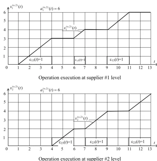
In the example given in Fig. 2, it can be observed that for a planned batch of 29 units, the flow time of the job is 3 days (starting at t=1 and ending at t=4), slack time is 8.75 days (subject to the due date 12.75 days). Fig. 3 depicts execution dynamics of two subsequent operations at the i-supplier level subject to three capacity availability time windows (εij=1).
From Fig. 4, processing times, idle times, completion quantities and times can be observed. ) ( ) 3 , 0 ( t uj
1 2 3 4 5 6 7 60 50 40 30 20 10 0 70 ) 1 , 0 ( x t, days 90 80 100 8 9 10 11 12 13 14 15 16 17 ) 1 , 0 ( a ) ( ) 3 , 0 ( t xj ) ( ) 1 , 0 ( t xj T0=1 day Tf=12.75 days
Fig. 2. Dynamics of job execution ) , 2 , 0 ( æ i x 1 2 3 4 5 6 7 12 10 8 6 4 2 0 14 t,days 16 8 9 10 11 12 13 14 15 16 17 1 ) , 2 , 0 ( æ i a ) , 2 , 0 ( æ i x ) , 2 , 0 ( 1) æ ( i x ) , 2 , 0 ( 1) æ ( i a i j=1 i j=1 i j=1
Fig. 3. Dynamics of operation execution
Constraints (2) and (3) describe the precedence relations for jobs and operations of jobs. Constraint (4) is the assignment constraint and relates to splitting and overlapping. Eq. (5) constrains the conditions for switching the control variables from 0 to 1.
) o ( 1
J (Eq. 7) characterizes the overall number of completed jobs at t = Tf . This is the performance indicator for
throughput ) o ( , , 2
J (Eq. 8) reflects the flow time for A
) o ( 3
J (Eq. 9) characterizes the makespan for all A
o) ( , , 4 i
J (Eq. 10) characterizes the lead-time for A
o) (
, 5 i
J (Eq. 11) is the waiting time of job A
) o ( 6
J (Eq. 12) characterizes the fullness of the job completion subject to the planned batch quantities at the end of the planning interval
) o ( 7
J (Eq. 13) expresses the total tardiness for all operations subject to penalty functions ~~i(æ), i.e.,
on-time-delivery (OTD)
4.3 Dynamic model of channel control (model Мk)
State of the channel C(i) at Bi characterizes the readiness of the channel to process the operationDæ(i,j).
The process model of channel control is as follows:
) 1 , ( æ ) 1 , ( æ ) , ( æ æ 1æ 1 ) 1 , ( æ æ æ ) 1 , ( æ
j i j i j i i m j s j i j i j i x x b u x i (14)
m i s j i o j i j i u u x 1æ 1 ) 1 , ( æ ) 2 , ( æ ) 2 , ( (15) Constraints: (16)
( ) 1, , 1æ 1 ) 1 , ( æ t j u n i s j i i (17)Start and end conditions:
(18) Objective functions:
1 1 1 1 1 ) 2 , ( ) 2 , ( ) ( 1 1 2 1 0 2 1 ( ) ( ) m m l l T T k f d x x J (19)
1 1 1 1 1 ) 2 , ( ) 2 , ( ) ( 2 1 2 1 1 2 ) ( ) ( m m l l f f x T T x J (20) } 1 , 0 { ) ( ; 0 (æ,1) ) 1 , ( æ ) 2 , 0 ( æ x x t ui j i j i j
x
O h
x
O h0() ()(T0) ; 1() ()(Tf) Parameters: ) , ( æ æ j i i
b is the setup time of a channel
Decision variables: ) ( ) 1 , ( æ t
xij is the state variable for the channel C(i) at Bj during the setup to prepare the channel for processing
) ( æ
i,j
D after completion the operation Dæ(i,j) ) ( ) 1 , ( æ t
uij is a control variable; ui(æj,1)(t)=1, if C(i) is in the setup process, ui(æj,1)(t)=0, otherwise ) ( ) 2 , ( t
xj is the state variable characterizing the process (run) time of a channel
Eqs (14) and (15) describe the dynamics of channel utilization. Eq. (14) describes the setup dynamics and Eq. (15) considers the process time of each channel subject to assignments (i.e., variable
u
i(æoj,2)=1) given with the operations control model Мo. Constraints (16) and (17) determine the setup sequence and conditions forset-ups at C(i). Similar to the operations control model Мo, h(0),h1() are known differential functions for starting
and end conditions for the state vector х() = u1111(,1),...,u(msml,1),u11(,2),...,uml(,2) т.
Objective functions (19) and (20) can be used to estimate the equality of channel utilization (e.g., as a re-quirement to equal loading of suppliers and their capacities subject to a SC collaboration agreement) at
t (T0, Tf ] and at the end of the planning interval. 4.4 Dynamic model of resource control (model Мr)
Process model of resource control:
m i s j i j i j i j i u u d x 1æ 1 ) 1 , ( æ ) 2 , o ( æ ) ( æ ) 1 , p ( (21)
m i s j i j i j i j i u u g x 1æ 1 ) 1 , ( æ ) 2 , o ( æ ) ( æ ) 2 , p ( (22)
m i s j j i j i j i j i u u u d x 1æ 1 ) 1 , p ( ) 1 ( ) 1 , ( æ ) 2 , o ( æ ) ( æ ) 1 , p ( (23)
m i s j j i j i j i j i u u u g x 1æ 1 ) 2 , p ( ) 1 ( ) 1 , ( æ ) 2 , o ( æ ) ( æ ) 2 , p ( (24) ) 2 , p ( ) 4 , p ( ) 1 , p ( ) 3 , p ( ; j j j j u x u x (25) Constraints:
~( )( ) æ, , ) 1 , ( æ ) 2 , o ( æ ) ( æ u u H t d j i i j i j i j
(26)
f f T T j i T T j i j i j i u u d H d g 0 0 ) ( ~ ~ ) ( ) ( ( ) æ, , ) 1 , ( æ ) 2 , o ( æ ) ( æ (27)
(p,3() 1) (p,3() 1)
0, (p,1) (p,1) 0 ) 1 , p ( j j j j j a x u x u (28)
(p,4() 1) (p,4() 1)
0
,
(p,2) (p,2)0
) 2 , p (
j j j j ja
x
u
x
u
(29) (30)Start and end conditions:
(r)( 0)
; 1(r)
(r)( )
0 r) ( 0 x T O h x Tf h (31) Objective function:
j l j j x J 1 ~ 1 ) 3 , p ( ) p ( 1 (32) (33) Parameters: ) ( æ j id , gi(æj) are given consumption intensities of S( j) and N( j) for Dæ(i,j) and C( j)
) ( ~( ) t
Hj ,H~~(j)(t) are known intensities for recovery of S( j) and N( j), respectively ) 4 , p ( ) 1 ( ) 3 , p ( ) 1 ( , j j a
a are known volumes (quantities) of resource recovery at recovery cycle (–1)
,~~
~ are numbers of total recovery cycles
Decision variables: ) ( ) 1 , p ( t
xj ,x(jp,2)(t),x(jp,1)(t),x(jp,2)(t) are state variables that characterize the current quantity (volume) of:
(1) non-storable resources S( j) (2) storable resources N( j)
(3) non-storable and recoverable (at stages and ) resources
(4) storable and recoverable (at stages and ) resources subject to channel C( j) These state variables characterize π-resource dynamics, degradation and recovery.
) ( ) 3 , p ( t
xj , x(jp,4)(t) are auxiliary state variables needed to define the sequence of resource replenishment and the ends of the replenishment intervals, respectively.
~ ~ ,..., 1 ; ~ ,..., 1 }, 1 , 0 { ) ( ), ( (p,2) ) 1 , p ( t u t uj j
j l j jx
J
1 ~ ~ 1 ) 4 , p ( ) p ( 2) 2 , p ( ) 1 , p (
,
j ju
u
are control variables characterizing the recovery process for non-storable and storable resources respectively;u
(jp,1),
u
(jp,2) are equal to 1 if π-resource is under recovery at t point of time, and are equal to 0, otherwise.Eqs. (21)-(25) describe the dynamics of resource consumption/degradation (Eqs. 21 and 22) and replenish-ment/recovery (Eqs 23 to 25) subject to assignment and setup decisions taken in models Мo and Мk.
According to constraints (26) and (27), if we have non-recoverable resources, H~(j), H~~(j) are interpreted as maximal resource consumption intensities at each point of time t.
Constraints (28)-(30) determine the sequence of replenishment/recovery actions. In other words, Eqs (21), (22), (26) and (27) describe the process of resource decrease and Eqs (23)-(25), (28)-(30) describe the process of resource replenishment/recovery policies.
The objective functions (32) and (33) can be introduced to estimate the fullness of resource replenishment and the timeliness of resource replenishment respectively. Eqs (32) and (33) can also be used to estimate the time-to-recovery, i.e., the time needed for resource regeneration.
4.5 Dynamic model of flow control (model Мf )
The interrelations and mutual impacts of the assignment and flow control still remain an open research ques-tion. In the proposed approach, these decisions are considered simultaneously. Recall that the lead-times (task times) may differ regarding different speeds
c
i(æfj,1) and channel availabilities
ij(t) and iæj(t). For instance, the assignment of an operation to two different channels could result in a different execution control profile and task time. For this reason, the assignments from the model Mo (made on the basis of the volumesa
i) are now subject to further optimization regarding the flow dynamics control.An assignment of an operation to a channel and the starting execution of the operations cause dynamic flows of the processed products. Let us introduce a model for the flow dynamics control (34):
Process model of flow control:
) 2 , f ( æ ) 2 , f ( æ ) 1 , f ( æ ) 1 , f ( æj i j
;
i j i j iu
x
u
x
; (34) Constraints: ) 2 , o ( æ ) 1 , f ( æ ) 1 , f ( æ0
u
i j
c
i ju
i j ; (35)
(æf,1) (æf,1)
0
;
(æf,2) (~æo,2)0
;
(æf,2)(
)
{
0
,
1
}
) 2 , f ( æa
x
u
x
u
t
u
i j i i j i j i i j ; (36)
(1) 1 1æ 1 1 ) 2 , f ( æ ) 2 , o ( æ ) 1 , f ( æ~
j m i l s k j i j i j iu
P
x
i i i
; (37) ) 2 ( 1 1æ 1 ) f,1 ( æ~
j m i l s j iP
u
i i
; (38) ) 3 ( 1æ 1 1 ) 1 , f ( æ~
ij l s k j iP
u
i i i
. (39)Start and end conditions:
x
O h
x
O h0(f) (f)(T0) ; 1(f) (f)(Tf) (40) Objective functions:
f i i i T t m i s m j i j l k j i i x a J
1æ 1 1 1 1 2 ) 1 , f ( æ ) 1 , f ( æ ) f ( 1 (41)
m i s m j i j l k T T j i i i i f d x J 1æ 1 1 1 1 ) 2 , f ( æ ) f ( 2 0 ) ( (42) Parameters: ) 1 , f ( æ ia
is known lot size of a product type for each operationDæ(i,j), , are known values for maximal storage capacity at Bj, handling capacity (throughput) at Bj for , and handling capacity (throughput) between Bi and Bj
) 1 , f ( æj i
c
is maximal processing intensity for the operation Dæ(i,j)at the λ-channel; it determines the maximal pos-sible value foru
i(æfj,1)Decision variables: ) ( ) 1 , f ( æ t
xi j is a state variable characterizing a quantity (volume) of the product «» being delivered at Bj from Bi during the execution of Dæ(i,j) (or the processed quantity at Bj, if i = j)
) ( ) 2 , f ( æ t
xi j is auxiliary state variable characterizing total processing time (including waiting time) of a product flow resulted from interaction of Bi and Bj for Dæ(i,j) at C(i),C( j)
) 1 , f ( æj i
u
is shipment intensity for transportation from Bi to Bj (or processing intensity at Bj if i = j); ()) 2 , f ( æ t ui j is auxiliary control variable; ui(æf,j2)(t)=1, if processing at Bj is completed (ui(æf,j2)(t)=0, otherwise) or if after the completion of Dæ(i,j) (or Dæ(i), of i = j), the next operation in the technological processDæ~(i,j) (or Dæ~(i), if i = j) begins.
Eq. (34) describes the flow dynamics. Eqs (35) and (37)-(39) constrains the maximal processing intensities subject to assignments in the model Мo. Eq. (15) considers the process time of each channel subject to
as-signments (i.e., variable
u
i(æoj,2)=1) from the operations control model Мo. Constraints (16) and (17) determinethe setup sequence and conditions for setups at C(i). Similar to operations control model Мo, h(0),h1() are
known differential function for starting and end conditions for state vector х() = = u1111(,1),...,umsml(,1),u11(,2),...,uml(,2) т. Objective function (41) characterizes the fullness of operations execution
) 1 ( ~ j P P~j(2) P~ij(3)
and is interconnected with the objective function (12) from Mo model. Objective function (42) characterizes
waiting time for operations execution and is interconnected with the objective function (11) from Mo.
5. Schedule computation procedure
Consider the relations between the models from Section 4 (Fig. 4) including some perturbation vectors ξ(t).
) o ( x ) f ( x ) f ( 0 x ) ( x ) r ( u ) o ( 0 x ξ(o) ) r ( 0 x ξ(r) Мr
М
Мo
Мf
) ( 0 x ξ() ) r ( x ) ( J ) ( u ) f ( u ) f ( ξ ) o ( 0 u ) o ( J ) (r J
Fig. 4. Model integration and introduction of uncertainty
Computation of schedule with the help of OPC is not a trivial problem. The computational procedure for the developed model is based on the integration of the main and conjunctive equation systems subject to the max-imization of Hamiltonian function. A methodical challenge in applying the maximum principle is to find the coefficients of the conjunctive system which change in dynamics. In the study (Ivanov et al. 2015) it has been shown that these coefficients can be found analytically. The coefficients of the conjunctive system play the role of the dynamical Lagrange multipliers as compared with discrete optimization dual formulations. Thus the transversality conditions establish the connection between the dual and direct problems.
The scheduling model in terms of OPC may be represented in the following form:
, 0 ) , ( , 0 ) , ( , 0 )) ( ( , 0 )) ( ( ), , , ( | ) ( ) 2 ( ) 1 ( 1 0 0 u x q u x q x h x h u x f x u f T T t t M (43)
where h0,h1 are given functions of end conditions at time tT0,t Tf and
(1) (2)
,
q
q
is the generalized notation of the linear and non-linear constraints, respectively.The presented models have four features that distinguish them from classical optimal control problems. First, the right parts of differential equations in Mo model are broken not only during the assignment selections but
also at the beginning of transportation operations. Second, we consider multi-objective formulation. Third, perturbations (disturbances) are considered in different models. Fourth, and probably, the most important,
non-linearity is transferred to the constraints; therefore process control models are linear (apart from flow and channel control models that are bi-linear).
In this setting, at the moment t = T0 we have some start conditions h0(x(t)) G
~
m
R and it becomes possible to find both optimal program control vector u*(t) and state vector х* at t = T0. Assuming that partial objective
functions can be converted to a general performance indicator JG, we have:
f f T T T T f f d f d T J 0 0 ) ( ) ( ) ( 2 G(1) 3 G(2) G 1 G x x u , (44)where 1>0,2>0,3>0, are given weight coefficients, G, fG(1), fG(2) are given functions at
X RnG, X T, U RmG (T = R+ is the set of time moments, R+ is a set of real numbers , X, U are sets for х, u). Assume that G(х) has no interruptions for Х, fG(1)(x(),) along with its derivative for х at each
(T0, Tf] has no interruptions for х and is piecewise-continuous at х Х for ; fG(2) for each is convex regarding u and for each u U it is bounded and piecewise-continuous for t. In the model M (43), we con-sider along with the feasible control class K~ and extended feasible control class K~~, where the relay condi-tion:
0
;
1
)
(
) (
t
u
ioj (45)is replaced by a less strict one:
0
;
1
)
(
) (
t
u
ioj (46)In this case, an extended domain
( )
~ ~t
x
Q of feasible control inputs may be formed by means of special trans-formations ensuring the convexity and the compactness of Q
x(t)
(Moiseev, 1974).Remark. Note that the constraints (2)–(5) and (35)–(39) are identical to those in the MP models for
schedul-ing. However, at each t-point of time, the number of variables in the calculation procedure is determined by the operations which are currently in the “active zone” of scheduling (Ivanov et al., 2015). For the problem sizes subject to the “active zone”, known methods for the solution of the MP models (e.g., the Hungarian method for Mo or linear programming (LP) for Mf) can be applied.
Let us consider the algorithmic realization of the above-described modified maximum principle. After trans-forming into a boundary problem, a relaxed problem can be solved to receive an OPC, for the computation of which the main and conjunctive systems are integrated, i.e., the OPC vector
u
*(
t
)
and the state trajectory)
(
*t
x
are obtained. The OPC vector at time t = T0 returns the maximum to objective functions, which havebeen transformed to a general performance index and expressed in scalar formJ . G
The basic peculiarity of the boundary problem considered is that the initial conditions for the conjunctive var-iables (t0) are not given. At the same time, an OPC should be calculated subject to the start and end
condi-tions. To obtain the conjunctive system vector, we use the Krylov–Chernousko method of successive approx-imations (MSA) for an OPC problem with a free right end which is based on the joint use of a modified suc-cessive approximation method (Krylov & Chernousko, 1972). We propose to use a heuristic schedule u(t) to obtain the initial conditions for (t0). Then, the algorithm can be stated as follows:
1 3 1
i iStep 1 An initial solution u(t),t(T0,Tf] (a feasible schedule) is selected and r0.
Step 2 As a result of the dynamic model run, x(r)(t) is received. Besides, if t Tf then the record value )
(r
G G J
J can be calculated. Then, the transversality conditions are evaluated.
Step 3 The conjugate system is integrated subject to u(t)u(t) and over the interval from t Tf to
t
T
0.Here, the iteration number
r
0
is completed.Step 4 From the time point
t
T
0 onwards, the control u(r 1)(t) is determined (r0,1,2,...denotes the num-ber of the iteration). In parallel with the maximization of the Hamiltonian, the main system of equations and the conjugate one are integrated. The maximization involves the solution of several MP problems at each time point.In the result, the assignment of jobs to suppliers and definition of the starting and end time for processing an operation on the channels at the supplier results automatically from the OPC vector u(t)u(t) subject to the assignment control variables (cf. Figs 2 and 3). The assignments (i.e., the control variablesui(æo,j2,)(t)) from the model Mo are used in the channel control model Mk , resource control model Mr and flow control Mf by means of the constraints (16), (26), (27), (35-37), respectively. At the same time, the model Mf influences the model Mo through the transversality conditions, the conjunctive system, and the Hamiltonian function. In addition, the possible resource structure dynamics and flow control dynamics through perturbation impacts can be taken into account including some perturbation vectors ξ(t) in supply constraints (26)-(27) and capacity constraints (37-(39).
6. Robust schedule coordination control
Consider the model (47) under the disturbances
ξ
( )
t
: 0 ) , , ( , 0 ) , , ( , 0 )) ( ( , 0 )) ( ( ), , , ( | ) ( ) 2 ( ) 1 ( 1 0 0 u x q u x q x h x h u x f x u f T T t t M (47)
For a simplification, it is assumed that the transition from the vector form
J
to a scalar formJ
G has been performed on the basis of the weight coefficients. Now the scheduling problem can be formulated as the fol-lowing problem of dynamic system control. The task is to find a feasible control u(t), [T0,Tf) which ensures that the dynamic control model meets the constraint functions and guides the dynamic system (i.e., the sched-ule) x f(t,x,u) from the initial state to the specified final state subject to given end conditions and the uncertainty area under the disturbancesξ
( )
t
. If there are several feasible controls (schedules), then the best one (optimal) should be selected in order to maximize (minimize) the components ofJ
G.Introduction of disturbance (perturbation) functions in constraints of the model (1)-(9) allows computing at-tainable sets (AS) of different feasible schedules, i.e., all possible results (i.e., throughout and tardiness) of the schedule execution subject to different variations of the parameters (e.g., the capacity disruptions). In other words, the introduction of AS opens a possibility to analyse the performance variations in feasible schedule execution policies under conditions of non-stationary perturbations (Chernousko 1994, Ivanov and Sokolov
2010). Since we consider a SC scheduling problem, we integrate the coordination issues into robustness analysis.
Assume that a certain initial state of x(T0) is known and that a schedule u*l(t) has been calculated. Then, an AS can be brought into correspondence with the vectors x(T0), ul(t), and j(t). ξ(t) is a perturbation vector at the moment
t
,
is a set of allowable perturbations ξ1(t)ξ(t)ξ2(t). ξ1(t ξ), 2(t)are prescribed vector functions, which define minimum and maximum values of perturbation effects on the realization stage for each fixed schedule.Let us introduce notation for AS.Dx(t,T0,x(T0),U(x(T0))) is an AS in the state space, ))) ( ( ), ( , , (t T0 T0 T0 J x U x
D is an AS in the performance indicators’ space, DJξ(t,T0,x(T0),,U(x(T0)))is an approximated AS under disturbances at the moment
t
.This AS represents the set of all possible execution scenarios which may occur in the schedule execution after the perturbations. We propose this area to be named as the AS in the state space under disturbances defined as follows: ) , , , , ( 0 0 ) ( l f x T T X D u (48) where l is the number of a feasible schedule.
As the dimensionality of the AS is high, the construction of an AS is a rather complicated problem. That is why an AS is usually approximated in different forms. Let us denote Dx(Tf,T0,x(T0),U(x(T0))) as an
approx-imation of AS Dx(Tf,T0,x(T0),U(x(T0))). Let us introduce the algorithm of
construction (Chernousko 1988) and exemplify it via the model (1). Using AS, it becomes possible to formu-late a dual problem:
)) ( , , ( ) ( G 0 0 ˆ min )) ( ( T T T Di f J x x x , (49)
where Diˆ(Tf,T0,x(T0)) is AS of Miˆ ( iˆ = 1,2,3); JG x( ()) the terminal functional subject to Eq. (44). One possible method for construction D(Tf,T0,x(T0)) is multiple solution of the problem (50):
) ( ~ т G( ()) ( ) min x u x c x Q f T J , (50)
The boundary points of the set Dx(Tf,T0,x(T0),U(x(T0))) are obtained as the solutions to Eq. (50), where c is a intended vector such that c 1. For each vector c we obtain the OPC u*(t), state x*(Tf) as one boundary point of and the hyperplane cTx*(Tf).
Let
c be the number of different vectorsc
,
,...,
1
c, then the external approximation ))) ( ( ), ( , , (Tf T0 T0 T0 x x U xD of the set Dx(Tf,T0,x(T0),U(x(T0))) is a polyhedron whose faces lie on the corresponding hyperplanes, and the internal approximation Dx(Tf,T0,x(T0),U(x(T0)))
is a polyhedron whose vertices are the points x*(Tf),1,...,c, i.e. D (Tf,T0, (T0)) C0( 1(Tf),..., (Tf))
c x x x . ))) ( ( ), ( , , (Tf T0 T0 T0 x x U x D ))) ( ( ), ( , , (t T0 T0 T0 x x U x D
Consider an example of how to use AS to analyse the impact of schedule coordination of two suppliers В1 and В2 on the lead-time and work-in process of a customer order A3 subject to disruptions and recovery, state
vari-able and objective functions (9) and (12). Consider three situations: Full coordination, no disruptions
Capacity disruption at supplier #2 and supply disruption from the supplier #2 Partial capacity recovery at supplier #2 and coordination of the schedules
In Fig. 5, the initial situation of full coordination without any disruptions is represented.
13(t)=1 1 2 3 4 5 6 7 6 5 4 3 2 0 t 8 9 1 ) ( ) 2 , o ( 1 t x 6 ) ( ) 2 , o ( 1 t a 10 11 12 13 13(t)=1 13(t)=1 ) ( ) 2 , o ( 1 t x
Operation execution at supplier #1 level
1 2 3 4 5 6 7 6 5 4 3 2 0 t 8 9 1 ) ( ) 2 , o ( 2 t x 6 ) ( ) 2 , o ( 2 t a 10 11 12 13 23(t)=1 23(t)=1 ) ( ) 2 , o ( 2 t x 23(t)=1
Operation execution at supplier #2 level
Fig. 5. Job execution for full coordination without disruptions
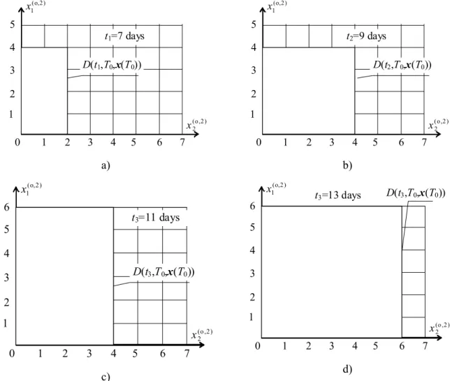
In Fig. 6, the corresponding AS employment in time is depicted.
)
(
) 2 , o ( 1t
x
) 2 , o ( 1 x ) 2 , o ( 2 x 1 2 3 4 5 6 7 5 4 3 2 0 1 D(t1,T0,x(T0)) t1=7 days a) ) 2 , o ( 1 x ) 2 , o ( 2 x 1 2 3 4 5 6 7 5 4 3 2 0 1 D(t2,T0,x(T0)) t2=9 days b) ) 2 , o ( 1 x ) 2 , o ( 2 x 1 2 3 4 5 6 7 5 4 3 2 0 1 D(t3,T0,x(T0)) t3=11 days 6 c) ) 2 , o ( 1 x ) 2 , o ( 2 x 1 2 3 4 5 6 7 5 4 3 2 0 1 D(t3,T0,x(T0)) t3=13 days 6 d)
Fig. 6. AS employment in time for full coordination without disruptions
From Figs 5-6 it can be observed that operation execution at both suppliers is completed fully subject to the planned lot-size of 6 units. The completion time is 11 days at supplier #1 and 13 days at supplier #2.
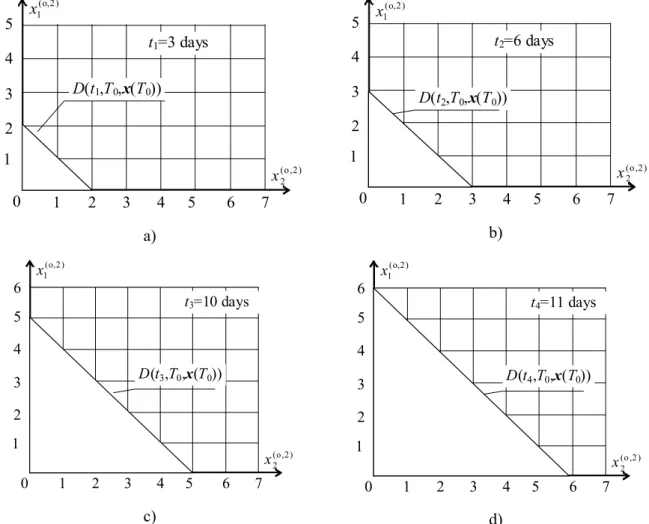
In the second situation, we have capacity disruption at supplier #2 and supply disruption from the supplier #2 (Fig. 7). 1 2 3 4 5 6 7 6 5 4 3 2 0 t 8 9 1 ) 2 , o ( 1 x 10 11 12 13 13(t)=1 13(t)=1 ) ( ) 2 , o ( 1 t x 13(t)=1 0 ) ( ) 2 , o ( 2 t x
Fig. 7 Operation execution at supplier ‘1 and capacity disruption at supplier #2 In Fig. 8, the corresponding AS employment in time is depicted.