Universal short time g*-functions : generation and application

(1)

Titre:

Title

: Universal short time g*-functions : generation and application

Auteurs:

Authors

: Michel Bernier et Yves Brussieux

Date: 2019

Type:

Article de revue / Journal article

Référence:

Citation

:

Bernier, M. & Brussieux, Y. (2019). Universal short time g*-functions : generation and application. Science and Technology for the Built Environment, 25(8), p. 993-1006. doi:10.1080/23744731.2019.1648132

Document en libre accès dans PolyPublie

Open Access document in PolyPublie

URL de PolyPublie:

PolyPublie URL: https://publications.polymtl.ca/4088/

Version: Version finale avant publication / Accepted version_{Révisé par les pairs / Refereed} Conditions d’utilisation:

Document issued by the official publisher

Titre de la revue:

Journal Title: Science and Technology for the Built Environment, 25(8) Maison d’édition:

Publisher: Taylor & Francis URL officiel:

Official URL: https://doi.org/10.1080/23744731.2019.1648132 Mention légale:

Legal notice:

This is an Accepted Manuscript of an article published by Taylor & Francis in Science and Technology for the Built Environment, 25(8)] on 2019, available online: http://www.tandfonline.com/10.1080/23744731.2019.1648132

Ce fichier a été téléchargé à partir de PolyPublie, le dépôt institutionnel de Polytechnique Montréal

This file has been downloaded from PolyPublie, the institutional repository of Polytechnique Montréal

(2)

Full Terms & Conditions of access and use can be found at

https://www.tandfonline.com/action/journalInformation?journalCode=uhvc21

Science and Technology for the Built Environment

ISSN: 2374-4731 (Print) 2374-474X (Online) Journal homepage: https://www.tandfonline.com/loi/uhvc21

**Universal short time g*-functions: generation and**

application

Yves Brussieux & Michel Bernier

To cite this article: Yves Brussieux & Michel Bernier (2019): Universal short time

g*-functions: generation and application, Science and Technology for the Built Environment, DOI: 10.1080/23744731.2019.1648132

To link to this article: https://doi.org/10.1080/23744731.2019.1648132

Accepted author version posted online: 31 Jul 2019.

Submit your article to this journal

(3)

1

Universal short time g

*

_{-functions: generation and application}

Yves Brussieux, Michel Bernier

Ecole Polytechnique de Montreal, Montreal, Quebec, Canada

Corresponding author Michel Bernier

[email protected]

ABSTRACT

A hybrid numerical/analytical one-dimensional model is proposed to predict the thermal behavior of borehole heat exchangers in the short period following a step change in operating conditions. Transient heat transfer in the borehole is solved numerically using an equivalent composite cylinder geometry while ground heat transfer is evaluated analytically using the infinite cylindrical heat source solution. The proposed model is then used to generate 𝑔∗_{-functions, which are based on a slightly different definition than the traditional g-functions. For short} times, 𝑔∗-functions depend on four non-dimensional parameters: 2𝜋𝑘𝑔𝑅𝑏, 𝑡/𝑡𝑐 (with 𝑡𝑐 equal to a new characteristic time) and 𝑁𝑓 and 𝑁𝑔, non-dimensional parameters related to the fluid and the ground, respectively. A set of universal 𝑔∗_{-functions curves generated with the proposed model is presented. Then, these curves are} used in a borehole sizing problem. It is shown that the inclusion of borehole thermal capacity has a direct effect on the daily and monthly effective ground thermal resistances which reduces the required borehole length by a few percent.

Keywords geothermal; g-functions; Thermal capacity INTRODUCTION

So-called g-functions are used extensively in the design and simulation of vertical ground heat exchangers

Accepted Manuscript

[email protected]

Accepted Manuscript

[email protected]

dimensional model

Accepted Manuscript

dimensional model is proposed to predict

Accepted Manuscript

is proposed to predict heat exchangers in the short period following a step change in operating conditions

Accepted Manuscript

heat exchangers in the short period following a step change in operating conditions using an equivalent composite cylinder geometry

Accepted Manuscript

using an equivalent composite cylinder geometry evaluated analytically using the infinite cylindrical heat source solution.

Accepted Manuscript

evaluated analytically using the infinite cylindrical heat source solution. functions, which are based on a slightly different definition

Accepted Manuscript

functions, which are based on a slightly different definition four non

Accepted Manuscript

four

non-Accepted Manuscript

-dimensional parameters:

Accepted Manuscript

dimensional parameters: and

Accepted Manuscript

and 𝑁

Accepted Manuscript

𝑁_𝑔

Accepted Manuscript

𝑔 𝑁_𝑔 𝑁

Accepted Manuscript

𝑁_𝑔 𝑁 , non

Accepted Manuscript

, non

Accepted Manuscript

-Accepted Manuscript

-dimensional parameters related to the fluid and the ground, respectively.

Accepted Manuscript

dimensional parameters related to the fluid and the ground, respectively. functions

Accepted Manuscript

functions curves generated with the proposed model is presented.

Accepted Manuscript

curves generated with the proposed model is presented. sizing problem. It is shown

Accepted Manuscript

sizing problem. It is shown

on the daily and monthly effective ground thermal resistances which

Accepted Manuscript

on the daily and monthly effective ground thermal resistances which

Keywords geothermal; g

Accepted Manuscript

(4)

2

(VGHE). g-Functions are thermal response factors that give the non-dimensional temperature drop at the borehole wall due to a constant total heat extraction rate in a borehole field. Traditional (or long-time) g-functions depend on four non-dimensional parameters: 𝑡/𝑡𝑠, the non-dimensional time, with 𝑡𝑠 = 𝐻2/9𝛼 , the characteristic time of the bore field and 𝛼 the ground thermal diffusivity; 𝑟𝑏/𝐻 the non-dimensional borehole radius; 𝐵/𝐻 the bore field aspect ratio; and 𝐷/𝐻 the non-dimensional buried depth of the boreholes. As shown in Figure 1, g-function curves are typically plotted as a function of 𝑙𝑛(𝑡/𝑡𝑠). For large values of 𝑙𝑛(𝑡/𝑡𝑠), g-function curves depend largely on the non-dimensional borehole spacing, 𝐵/𝐻. These curves merge into a single curve with a decrease in the value of 𝑙𝑛(𝑡/𝑡𝑠). The original (or long-time) g-functions obtained by Eskilson (1987) did not cover time periods of less than a month. As reported by Yavuzturk and Spitler (1999), Hellström extended the g-functions so that they could be used down to about 100 hours. For a typical borehole, this represents a value of 𝑙𝑛(𝑡/𝑡𝑠) ≈ -9. It is possible to extend g-function curves below this value using the infinite line source solution for example. One such curve (indicated by an arrow for 𝐵/𝐻 = ∞) is presented in Figure 1. However, this curve does not account for short-time transient effects due to the borehole thermal capacity.

Figure 1 Short-time and long-time g-functions on the same non-dimensional time scale

Yavuzturk and Spitler (1999) were the first to extend the concept of g-functions to short time steps taking into account the pipe and grout thermal capacities but neglecting the fluid thermal capacity. Xu and Spitler (2006) extended this work by approximating the U-tube geometry with a series of hollow cylinders representing the fluid, the internal convective resistance, the pipe, the grout and the ground. They have shown that results obtained with

Accepted Manuscript

curves merge into a single curve with a decrease in

Accepted Manuscript

curves merge into a single curve with a decrease in tions obtained by Eskilson (1987) did no

Accepted Manuscript

tions obtained by Eskilson (1987) did not cover time

Accepted Manuscript

t cover time Hellström extended the g

Accepted Manuscript

Hellström extended the

g-Accepted Manuscript

-functions so

Accepted Manuscript

functions so that they could be used down to about 100 hours. For a typical borehole, this represents a value of

Accepted Manuscript

that they could be used down to about 100 hours. For a typical borehole, this represents a value of 𝑙𝑛

Accepted Manuscript

𝑙𝑛 function curves below this value using the infinite line source solution

Accepted Manuscript

function curves below this value using the infinite line source solution ) is presented in Figure 1. However, this curve does

Accepted Manuscript

) is presented in Figure 1. However, this curve does

Accepted Manuscript

Figure 1

Accepted Manuscript

Figure 1 Short

Accepted Manuscript

Short

Yavuzturk and Spitler (1999) were the first to extend the concept of g

Accepted Manuscript

Yavuzturk and Spitler (1999) were the first to extend the concept of g

Accepted Manuscript

(5)

3

this technique compare favorably well with the ones obtained with a two-dimensional model representing the real borehole geometry. Brussieux and Bernier (2018) followed a similar approach for the borehole but used the cylindrical heat source solution to model transient effects in the ground. Using this approach, it is possible to calculate g-functions for short times. Three such curves are presented in Figure 1 for 𝑙𝑛(𝑡/𝑡𝑠) < -9. These curves are specific to certain borehole characteristics and are plotted using the same non-dimensional scale used for long-time g-functions.

In this paper, it is shown that it is possible to obtain universal short-time g-functions using four non-dimensional parameters: 2𝜋𝑘𝑔𝑅𝑏 , 𝑡/𝑡𝑐 , 𝑁𝑓 , 𝑁𝑔 . To avoid confusion with the standard g-function definition, the name has been changed to 𝑔∗-function. However, 𝑔∗-function are identical to standard g-functions for long times. Typical 𝑔∗_{-function curves are presented in Figure 2. Note that short-time 𝑔}∗_{-functions use the top scale based on} 𝑙𝑛(𝑡/𝑡𝑐) while long-time 𝑔∗-functions (to the right of the vertical line) use the bottom scale based on 𝑙𝑛(𝑡/𝑡𝑠). The objective of this paper is to show how to generate these universal short-time 𝑔∗_{-function curves and to} provide an example of their application.

Figure 2 Schematic representation of universal short-time 𝒈∗-function curves along with traditional long-time g-function.

Accepted Manuscript

using four non

Accepted Manuscript

using four non

function definition, the name

Accepted Manuscript

function definition, the name functions for long times. Typical

Accepted Manuscript

functions for long times. Typical function

Accepted Manuscript

functions

Accepted Manuscript

s use the top scale

Accepted Manuscript

use the top scale functions (to the right of the vertical line) use the bottom scale

Accepted Manuscript

functions (to the right of the vertical line) use the bottom scale these universal short

Accepted Manuscript

these universal

short-Accepted Manuscript

-time

Accepted Manuscript

time 𝑔

Accepted Manuscript

𝑔∗

Accepted Manuscript

∗

Accepted Manuscript

(6)

4

LITERATURE REVIEW

The impact of borehole thermal capacity on borehole heat transfer has been the subject of many investigations. Shirazi and Bernier (2013) provided a thorough review of the area up to 2013. Other studies, which were not reviewed by these authors, will now be discussed.

Yavuzturk et al. (2009) improved the approach developed by Yavuzturk and Spitler (1999) mentioned earlier. Their proposed model is one-dimensional (in the radial direction) and couples two different calculation domains. First, heat transfer in the borehole is solved with a finite element method where the borehole wall temperature is considered to be known. Secondly, ground heat transfer is solved with an analytical short time response factor based on the infinite cylindrical heat source. At each time step, an iterative method gives the fluid temperature based on the wall temperature obtained at the previous time step. The equivalent geometry used is the one developed by Gu and O’Neal (1998) except that the borehole thermal resistance is evaluated using the multipole method. The model is implemented in TRNSYS and validated against numerical and analytical models as well as experimental data. The model proposed here is based on a similar approach except that the equivalent geometry is different as well as the solution methodology. In addition, the proposed model goes one step further by proposing a method to generate and use short time 𝑔∗-functions.

Javed et al. (2010), Javed and Claesson (2011) and Claesson and Javed (2011) proposed an analytical one-dimensional model to simulate the short and long term thermal response of VGHE where the U-tube is replaced by a composite cylinder. Borehole heat transfer is solved in the Laplace domain with the use of a circuit of thermal resistances and then inverse transforms are used to revert back to the time domain. Lamarche (2015) used a similar approach and later used his solution to study the impact of short time effects on the required length of VGHE (Lamarche, 2016). He showed that for a particular case, the required borehole length could be overestimated by about 5% when short-term effects are neglected.

Li and Lai (2013) and Li et al. (2014) proposed a two-dimensional analytical model for U-tube boreholes in which each tube is replaced by an infinite line source. Their results match experimental data with good accuracy for times as short as several minutes. Ma et al. (2015) used a similar composite-medium line source but in three dimensions to account for the variation of fluid temperature along the U-tube. However, the fluid thermal capacity is not taken into account in these models.

Accepted Manuscript

developed by Yavuzturk and Spitler (1999)

Accepted Manuscript

developed by Yavuzturk and Spitler (1999) mentioned

Accepted Manuscript

mentioned two different

Accepted Manuscript

two different calculation

Accepted Manuscript

calculation domains.

Accepted Manuscript

domains. the borehole wall temperature

Accepted Manuscript

the borehole wall temperature , ground heat transfer is solved with an analytical short time response factor

Accepted Manuscript

, ground heat transfer is solved with an analytical short time response factor At each time step, an iterative meth

Accepted Manuscript

At each time step, an iterative method gives the fluid temperature

Accepted Manuscript

od gives the fluid temperature The equivalent geometry used is the one

Accepted Manuscript

The equivalent geometry used is the one e borehole thermal resistance

Accepted Manuscript

e borehole thermal resistance is evaluated using

Accepted Manuscript

is evaluated using odel is implemented in TRNSYS and validated against numerical and analytic

Accepted Manuscript

odel is implemented in TRNSYS and validated against numerical and analytic e model proposed here is based on a similar approach except that

Accepted Manuscript

e model proposed here is based on a similar approach except that

Accepted Manuscript

In addition, the proposed model goes one step further by proposing

Accepted Manuscript

In addition, the proposed model goes one step further by proposing functions.

Accepted Manuscript

functions.

Javed et al. (2010), Javed and Claesson (2011) and Claesson and Javed (2011) proposed an analytical one

Accepted Manuscript

Javed et al. (2010), Javed and Claesson (2011) and Claesson and Javed (2011) proposed an analytical one dimensional model to simulate the short and long term thermal response of

Accepted Manuscript

dimensional model to simulate the short and long term thermal response of

by a composite cylinder. Borehole heat transfer is solved in the Laplace domain with the use of a circuit of

Accepted Manuscript

by a composite cylinder. Borehole heat transfer is solved in the Laplace domain with the use of a circuit of thermal resistances and then inverse transforms are used to revert back to the time domain. Lamarche (2015) used

Accepted Manuscript

thermal resistances and then inverse transforms are used to revert back to the time domain. Lamarche (2015) used a similar approach and later

Accepted Manuscript

a similar approach and later used his solution to study the impact of short time effects on the required length of

Accepted Manuscript

used his solution to study the impact of short time effects on the required length of

Accepted Manuscript

(Lamarche, 2016)

Accepted Manuscript

(Lamarche, 2016). He showed that for a particular case, the required borehole length could be

Accepted Manuscript

. He showed that for a particular case, the required borehole length could be overestimated by about 5% when short

Accepted Manuscript

overestimated by about 5% when short

d Lai (2013) and Li et al. (2014) proposed a two

Accepted Manuscript

d Lai (2013) and Li et al. (2014) proposed a two

Accepted Manuscript

each tube is replaced by an infinite line source. Their results match experimental data with good accuracy for

Accepted Manuscript

each tube is replaced by an infinite line source. Their results match experimental data with good accuracy for

times as short as several minutes. Ma

Accepted Manuscript

(7)

5

Yang and Li (2014) proposed a new two-dimensional finite volume model considering the fluid capacity and used it to validate the previously developed composite medium line source model (Li and Lai, 2013) which did not consider fluid and pipe heat capacities. When compared with the sand box dataset of Beier (Beier et al. 2011), it is shown that the two models match very well except in the first minutes where the heat capacity affects the results. The influence of other parameters like shank spacing or thermal properties is also studied and once again, the two models differ only during the first minutes.

Li and Lai (2015) provided a discussion on several new advances of borehole heat exchangers analysis. A critical review of six analytical models is presented. The difficulty in providing a precise heat transfer model which covers different time scales is emphasized. Numerical model can be very precise, but they are computationally intensive and thus cannot be used efficiently for long simulations. Analytical models do not suffer from long computations but are based on more stringent assumptions which may limit their accuracy. Aside from the reference dataset of Beier et al. (2011), the authors also note the lack of experimental data to validate models. Li et al. (2017) proposed a new VGHE sizing equation taking into account the short-term thermal resistance and variation in the fluid temperature. The new effective thermal resistance is divided into a fluid-to-pipe resistance based on the work of Ma et al. (2015) and a pipe-to-ground thermal resistance based on the G-function concept developed by Li et al. (2014). The new sizing equation is compared with the original ASHRAE sizing equation (ASHRAE, 2015) and a simulation-based design tool from Cullin et al. (2015). When compared to the data of Cullin et al. (2015) the new sizing equation appears to be more accurate than the ASHRAE sizing equation. The authors performed a sensitivity study to determine the influence of each parameter on the calculated length. This analysis is particularly relevant when the uncertainty on thermal properties is important. The authors provided G-function curves in the form of G-charts to help the calculation of short time thermal resistances. However, it appears that these charts do not cover all possible borehole configurations and parameters.

De Rosa et al. (2014) compared their short-term Borehole to Ground (B2G) model to the Duct ground heat STorage (DST) model developed by Hellström (1989) and implemented in TRNSYS. The B2G model is based on a two-dimensional thermal resistance-capacity approach including vertical discretization of the borehole. Thermal properties of the pipe, grout and ground are considered but not the fluid capacity. The model is compared with experimental data from an operating ground source heat pump installed to provide heating and cooling of a university building. Results show that the B2G model is more accurate than the DST model for the prediction of the outlet temperature under on/off operating conditions. Ruiz-Calvo et al. (2015) describe more precisely the structure of the B2G model. The model is improved by adding new thermal resistances to better capture the

Accepted Manuscript

Li and Lai (2015) provided a discussion on several new advances of borehole heat exchangers analysis. A critical

Accepted Manuscript

Li and Lai (2015) provided a discussion on several new advances of borehole heat exchangers analysis. A critical a precise heat transfer

Accepted Manuscript

a precise heat transfer model which

Accepted Manuscript

model which but they are computationally

Accepted Manuscript

but they are computationally intensive and thus cannot be used efficiently for long simulations. Analytical models do not suff

Accepted Manuscript

intensive and thus cannot be used efficiently for long simulations. Analytical models do not suff may limit their accuracy

Accepted Manuscript

may limit their accuracy

the lack of experimental data to validate models.

Accepted Manuscript

the lack of experimental data to validate models. sizing equation taking into account the short

Accepted Manuscript

sizing equation taking into account the short

resistance is divided into a fluid

Accepted Manuscript

resistance is divided into a fluid round

Accepted Manuscript

round thermal

Accepted Manuscript

thermal resistance based on the G

Accepted Manuscript

resistance based on the G equation is compared with the original ASHRAE

Accepted Manuscript

equation is compared with the original ASHRAE based design tool from Cullin et al. (2015).

Accepted Manuscript

based design tool from Cullin et al. (2015). appears to be

Accepted Manuscript

appears to be more

Accepted Manuscript

more

sensitivity study to determine the influence of each parameter on the calculated length. This

Accepted Manuscript

sensitivity study to determine the influence of each parameter on the calculated length. This cularly relevant when the uncertainty on thermal properties is important. The

Accepted Manuscript

cularly relevant when the uncertainty on thermal properties is important. The G

Accepted Manuscript

G-Accepted Manuscript

-charts to help the calculation of short time

Accepted Manuscript

charts to help the calculation of short time charts do not cover all possi

Accepted Manuscript

charts do not cover all possible borehole configurations and parameters.

Accepted Manuscript

ble borehole configurations and parameters. De Rosa et al. (2014) compared

Accepted Manuscript

De Rosa et al. (2014) compared their

Accepted Manuscript

their short

Accepted Manuscript

short model

Accepted Manuscript

model developed by Hellström (1989) and implemented

Accepted Manuscript

developed by Hellström (1989) and implemented

dimensional

Accepted Manuscript

dimensional thermal resistance

Accepted Manuscript

thermal resistance

Accepted Manuscript

properties of the pipe, grout and ground are consider

Accepted Manuscript

properties of the pipe, grout and ground are consider

xperimental data

Accepted Manuscript

(8)

6

thermal interaction between the U-tube legs and convection heat transfer. However, it does not consider the fluid thermal capacity. The model is validated against two different step tests with a 260 m deep water-filled borehole. The tests compare experimental and simulated values of the outlet fluid temperature with a ten-hour heat injection period. Two main adjustment parameters are determined and optimized, the penetration depth and grout node positions. The model is then combined with long term g-functions (Ruiz-Calvo et al., 2016) to obtain a full-time scale model.

Minaei and Marefat (2017a) proposed a simplification to the well-known thermal resistance capacity model, which is based on a stiff system of equation that makes it unstable except for small time steps. In the resulting STRCM model, they merged the two-grout zones proposed in the original version of the model into a single one. When compared with the sand box data of Beier (Beier et al., 2011), the TRCM and STRCM give both accurate results except for very early times where the simplified version is less accurate. However, the loss in accuracy is balanced with a gain in stability since the STRCM model is based on a non-stiff differential equation. A three-dimensional version of the STRCM is also proposed where heat transfer is solved numerically inside the borehole and analytically outside, using the infinite cylindrical heat source solution. The borehole is divided vertically into slices and each slice is solved with the 2D STRCM model. Slices are linked with the corresponding heat flux entering/leaving slices. The simplicity, accuracy and stability of the STRCM model makes it easy to implement into a building simulation software. In a related study, Minaei and Marefat (2017b) used a similar STRCM approach to model heat transfer in a single or double U-tube geometry. Governing equations are solved with Laplace transform and results are compared with the experimental data of Beier (Beier et al., 2011). This model is used to generate short-time g-functions and the influence of several parameters are discussed.

Beier (2014) developed a transient analytical heat transfer model for thermal response tests (TRT). The model uses an equivalent radius to transform the two-pipe geometry into an equivalent cylinder. The equations are solved with Laplace transforms and the vertical temperature profile is also generated. The model is successfully validated against experimental data and it is shown that the vertical temperature prediction capability leads to a more accurate estimation of the borehole thermal resistance than with the traditional mean temperature approximation.

He et al. (2010) studied the difference between two-dimensional and three-dimensional models in the calculation of transient fluid transport and heat transfer in a BHE. They showed that the predictions of transient heat transfer in a borehole from 2D models is not accurate since these models cannot account for fluid transport along the U-tube. Three-dimensional models can alleviate this deficiency, but they are computationally intensive. Instead, the

Accepted Manuscript

known thermal resistance c

Accepted Manuscript

known thermal resistance capacity model

Accepted Manuscript

apacity model which is based on a stiff system of equation that makes it unstable except for small time steps.

Accepted Manuscript

which is based on a stiff system of equation that makes it unstable except for small time steps. In the resulting

Accepted Manuscript

In the resulting original version of the model into a single one

Accepted Manuscript

original version of the model into a single one and STRCM

Accepted Manuscript

and STRCM give both accurate

Accepted Manuscript

give both accurate is less accurate

Accepted Manuscript

is less accurate. However, the loss

Accepted Manuscript

. However, the loss STRCM model is based on a non

Accepted Manuscript

STRCM model is based on a

non-Accepted Manuscript

-stiff differential equation

Accepted Manuscript

stiff differential equation

heat transfer is solved numerically inside the borehole

Accepted Manuscript

heat transfer is solved numerically inside the borehole infinite cylindrical heat source solution

Accepted Manuscript

infinite cylindrical heat source solution. The borehole is divided vertically into

Accepted Manuscript

. The borehole is divided vertically into model

Accepted Manuscript

model.

Accepted Manuscript

. S

Accepted Manuscript

Slice

Accepted Manuscript

lices are linked

Accepted Manuscript

s are linked cy and stability of

Accepted Manuscript

cy and stability of the

Accepted Manuscript

the STRCM

Accepted Manuscript

STRCM In a related study,

Accepted Manuscript

In a related study, Minaei and Marefat (2017

Accepted Manuscript

Minaei and Marefat (2017 approach to model heat transfer in a single or double U

Accepted Manuscript

approach to model heat transfer in a single or double

U-Accepted Manuscript

-tube geometry. Governing equatio

Accepted Manuscript

tube geometry. Governing equatio Laplace transform and results are compared with

Accepted Manuscript

Laplace transform and results are compared with the

Accepted Manuscript

the

Accepted Manuscript

experimental data of Beier

Accepted Manuscript

experimental data of Beier functions and the influence of several parameters

Accepted Manuscript

functions and the influence of several parameters

transient analytical heat transfer model for thermal response tests (TRT). The model

Accepted Manuscript

transient analytical heat transfer model for thermal response tests (TRT). The model adius to transform the

Accepted Manuscript

adius to transform the two

Accepted Manuscript

two

solved with Laplace transforms and the vertical temperature pro

Accepted Manuscript

solved with Laplace transforms and the vertical temperature pro

validated against experimental data and it is shown that the vertical temperature

Accepted Manuscript

validated against experimental data and it is shown that the vertical temperature more accurate estimation of

Accepted Manuscript

more accurate estimation of the borehole thermal resistance than with the

Accepted Manuscript

the borehole thermal resistance than with the

approximation.

Accepted Manuscript

approximation.

Accepted Manuscript

He et al. (2010) studied the difference between two

Accepted Manuscript

(9)

7

authors propose an improved 2D model to reduce computation. This improved model discretizes the borehole into vertical cells with homogenous temperatures, which enables the prediction of the vertical temperature profile and short time non-linearity.

Rees and He (2013) built a 3D numerical model using a finite volume approach to study fluid transport effects for short and long-time scales. The model represents the real borehole geometry including the fluid capacity. It is verified with experimental data obtained at a facility at Oklahoma State University. Emphasis was placed on the study of nonlinearities in temperature and heat flux for short time scales or low flow rates. The model is not convenient to use for any simulation because it is computationally demanding but can be used as a reference to validate other models. Rees (2015) developed an extended two-dimensional model that solves heat transfer in each layer of a VGHE with a finite volume method. This calculation is combined with a pipe model that divides the borehole vertically into small tank volumes. With such divisions, the pipe boundary condition depends on the depth and can reflect the evolution of the fluid temperature along the borehole. The focus of their work is on short-time behavior and thus, grout, pipe and fluid thermal capacities are considered. Different results are compared for the validation against experimental data from Oklahoma State University facility and against a full 3D model. First, the outlet temperature is calculated for varying input temperature based on a sinusoidal profile with a large range of frequencies. For this test, only 3D and extended 2D models are compared. Then, monthly and hourly outlet temperatures are compared between experiments, extended 2D and 3D models. The model shows a good agreement with the 3D model for short times while being more computationally efficient.

Kim et al. (2014) used a hybrid model, numerical inside the borehole and g-functions in the ground, to account for borehole thermal capacity. They used an equivalent radius and a state model size reduction technique to limit computation time. The resulting hybrid-reduced (HR) model was compared to the DST model and with Type451, a double U-tube borehole model that accounts for borehole thermal capacity (Wetter and Huber, 1997). The results obtained with the HR model are in excellent agreement with the DST model in no thermal capacity mode and with Type 451 when thermal capacity is included. However, the HR model involves an elaborate process only applicable to a certain borehole geometry.

Parisch et al. (2015) accounted for the fluid and grout thermal capacities by adding an adiabatic pipe, which accounts for the borehole thermal capacity, upstream of a steady-sate borehole model. Simulations results in TRNSYS performed with this approach show significant improvements.

Biglarian et al. (2017) suggested a numerical model able to predict both short and long-time heat transfer from a single borehole. The inside of the borehole is modeled with a resistance-capacity network, including the fluid

Accepted Manuscript

. The model is not

Accepted Manuscript

. The model is not convenient to use for any simulation because it is computationally demanding but can be used as a

Accepted Manuscript

convenient to use for any simulation because it is computationally demanding but can be used as a reference to

Accepted Manuscript

reference to dimensional model that solves heat transfer in

Accepted Manuscript

dimensional model that solves heat transfer in GHE with a finite volume method. This calculation is combined with a pipe model that divides

Accepted Manuscript

GHE with a finite volume method. This calculation is combined with a pipe model that divides , the pipe boundary condition depends on the

Accepted Manuscript

, the pipe boundary condition depends on the depth and can reflect the evolution of the fluid temperature along the borehole. The focus of

Accepted Manuscript

depth and can reflect the evolution of the fluid temperature along the borehole. The focus of

al capacities are considered. Different results are

Accepted Manuscript

al capacities are considered. Different results are against experimental data from Oklahoma State University

Accepted Manuscript

against experimental data from Oklahoma State University

for varying input temperature based on a

Accepted Manuscript

for varying input temperature based on a

a large range of frequencies. For this test, only 3D and extended 2D models are compared. Then, monthly

Accepted Manuscript

a large range of frequencies. For this test, only 3D and extended 2D models are compared. Then, monthly and hourly outlet temperatures are compared between experi

Accepted Manuscript

and hourly outlet temperatures are compared between experiments

Accepted Manuscript

ments, extended 2D and 3D mod

Accepted Manuscript

, extended 2D and 3D mod a good agreement with the 3D model for short time

Accepted Manuscript

a good agreement with the 3D model for short times

Accepted Manuscript

s while being more computationally efficient.

Accepted Manuscript

while being more computationally efficient. (2014) used a hybrid model, numerical inside the borehole and

Accepted Manuscript

(2014) used a hybrid model, numerical inside the borehole and

y. They used an equivalent radius and a state model size reduction technique to limit

Accepted Manuscript

y. They used an equivalent radius and a state model size reduction technique to limit hybrid

Accepted Manuscript

hybrid-Accepted Manuscript

-reduced (HR)

Accepted Manuscript

reduced (HR) tube borehole model

Accepted Manuscript

tube borehole model that

Accepted Manuscript

that accounts for borehole therma

Accepted Manuscript

accounts for borehole therma results obtained with the HR model are in excellent agreement w

Accepted Manuscript

results obtained with the HR model are in excellent agreement w and with Type 451 when thermal capacity is included

Accepted Manuscript

and with Type 451 when thermal capacity is included only applicable to a certain borehole geometry

Accepted Manuscript

only applicable to a certain borehole geometry

Parisch et al. (2015) accounted for the fluid and grout thermal capacities by adding an adiabatic pipe, which

Accepted Manuscript

Parisch et al. (2015) accounted for the fluid and grout thermal capacities by adding an adiabatic pipe, which

Accepted Manuscript

accounts for the borehole thermal capacity, upstream of a steady

Accepted Manuscript

(10)

8

capacity, and the outside with a finite volume method. A non-uniform grid is used to find a good balance between accuracy and computation time. Results compare favourably well with the experimental data of Beier (Beier et al., 2011), the 3D numerical model of Lee and Lam (2008) and the composite-medium line-source model of Li and Lai (2013).

Nian and Cheng (2018) proposed a new thermal response factor to account for borehole heat capacity. A 1D analytical model transforms the borehole geometry into an equivalent composite cylinder and solves the heat transfer with Laplace transforms. The fluid heat capacity, which is not included at first, is then included with a specific function either for U-tube or coaxial boreholes. The effect of borehole heat capacity and borehole radius on short time g-functions are studied and new g-functions are proposed. They compared favorably well with traditional g-functions and with the experimental data of Beier et al. (2011). However, the influence of conductivities and shank spacing on the response factor is not studied.

As shown by this survey of the literature, there are many ways to model short-time effects associated with borehole thermal capacity. However, unlike the non-dimensional long-time g-function curves, there are no “universal” pre-calculated curves that could be used to account for short-term effects. The objective of this paper is to propose a method to generate such non-dimensional short-time g-function curves.

The paper starts with a presentation of the governing equations and solution methodology followed by a validation of the proposed model against experimental data. Then, the governing non-dimensional parameters for short-time 𝑔∗-function are introduced and universal 𝑔∗-function curves are presented. In the application section of the paper, the ASHRAE sizing equation for VGHE is used in conjunction with short-time 𝑔∗_{-function to show} the impact of borehole thermal capacity on sizing.

PROPOSED MODEL

The following model is based on the equivalent geometry proposed by Xu and Spitler (2006) and illustrated in Figure 3. The two-pipe geometry, with a borehole radius 𝑟𝑏, is converted into a composite cylinder configuration

with the same borehole radius. The outer pipe radius of the equivalent geometry, 𝑟𝑒𝑞,𝑜𝑢𝑡,𝑝 , is set equal to √2 𝑟𝑜𝑢𝑡.

This ensures that the volume occupied by the grout is the same in both the real and equivalent geometries.

The inner pipe radius of the equivalent geometry, 𝑟𝑒𝑞,𝑖𝑛,𝑝, is set equal to 𝑟𝑒𝑞,𝑜𝑢𝑡,𝑝 minus the pipe thickness ∆

(= 𝑟𝑜𝑢𝑡− 𝑟𝑖𝑛). Then, a mass-less convection layer with a thickness of 0.25 × ∆ followed by a fully-mixed fluid

layer with a thickness of 0.75 × ∆ are used as suggested by Xu and Spitler (2006). Test performed indicated that

Accepted Manuscript

transfer with Laplace transforms. The fluid heat capacity, which is not included at first, is then included with a

Accepted Manuscript

transfer with Laplace transforms. The fluid heat capacity, which is not included at first, is then included with a al boreholes. The effect of borehole heat capacity and borehole radius

Accepted Manuscript

al boreholes. The effect of borehole heat capacity and borehole radius functions are proposed. They compared favorably well with

Accepted Manuscript

functions are proposed. They compared favorably well with functions and with the experimental data of Beier et al. (2011).

Accepted Manuscript

functions and with the experimental data of Beier et al. (2011). However, the influence of

Accepted Manuscript

However, the influence of As shown by this survey of the literature, there are many ways to model short

Accepted Manuscript

As shown by this survey of the literature, there are many ways to model

short-Accepted Manuscript

-time effects associated with

Accepted Manuscript

time effects associated with dimensional long

Accepted Manuscript

dimensional

long-Accepted Manuscript

-time g

Accepted Manuscript

time

g-Accepted Manuscript

-function

Accepted Manuscript

function calculated curves that could be used to account for short

Accepted Manuscript

calculated curves that could be used to account for

short-Accepted Manuscript

-term effects. The objective of this paper

Accepted Manuscript

term effects. The objective of this paper dimensional short

Accepted Manuscript

dimensional

short-Accepted Manuscript

-time g

Accepted Manuscript

time

g-Accepted Manuscript

-function curves.

Accepted Manuscript

function curves.

a presentation of the governing equations and solution methodology

Accepted Manuscript

a presentation of the governing equations and solution methodology against experimental data.

Accepted Manuscript

against experimental data. Then, the governing non

Accepted Manuscript

Then, the governing non nd universal

Accepted Manuscript

nd universal 𝑔

Accepted Manuscript

𝑔∗

Accepted Manuscript

∗

-Accepted Manuscript

-function curves

Accepted Manuscript

function curves

of the paper, the ASHRAE sizing equation for VGHE is used in conjunction with short

Accepted Manuscript

of the paper, the ASHRAE sizing equation for VGHE is used in conjunction with short the impact of borehole thermal capacity on sizing.

Accepted Manuscript

the impact of borehole thermal capacity on sizing.

Accepted Manuscript

he following model is based on the equivalent geometry

Accepted Manuscript

he following model is based on the equivalent geometry The two

Accepted Manuscript

The

two-Accepted Manuscript

-pipe geometry

Accepted Manuscript

pipe geometry

Accepted Manuscript

with the same borehole radius

Accepted Manuscript

with the same borehole radius

This ensures that the volume occupied by the grout is the same in both the real and equivalent

Accepted Manuscript

This ensures that the volume occupied by the grout is the same in both the real and equivalent

(11)

9

results were not significantly affected by a variation of these two thicknesses. An additional radius, 𝑟𝑓𝑎𝑟 , is used

by Xu and Spitler (2006) to set the far-field radius in the ground for their numerical model. This radius is not required here since ground heat transfer is handled with an analytical solution. An equivalent fluid thermal capacity, 𝜌𝐶𝑝𝑒𝑞,𝑓, is determined based on the actual fluid thermal capacity, 𝜌𝐶𝑝𝑓, as follows:

(𝜌𝐶𝑝)𝑒𝑞,𝑓=

2𝑟𝑖𝑛2

(𝑟_{𝑒𝑞,𝑖𝑛,𝑐}2 _{− 𝑟} 𝑒𝑞,𝑓2 )

(𝜌𝐶𝑝)𝑓 (1)

The local fluid is at a temperature equal to the average borehole fluid temperature, 𝑇𝑓, while the undisturbed ground temperature is given by 𝑇𝑔. The steady-state borehole thermal resistance,𝑅𝑏, is equal for both the real and equivalent geometries. It is determined here using the first order multipole method (Hellström, 1991) based on the real geometry. Once the value of 𝑅𝑏 is known, each layer is assigned equivalent properties as shown in Table 1. Governing equations and boundary conditions

One-dimensional transient heat transfer in the composite cylinder is governed by the following equation:

𝜌𝐶𝑝 𝜕𝑇 𝜕𝑡 = 𝑘 1 𝑟 𝜕 𝜕𝑟(𝑟 𝜕𝑇 𝜕𝑟) (2)

where 𝜌, 𝐶𝑝 and 𝑘 are the density, specific heat and thermal conductivity, respectively. This equation is subjected

to the following initial and boundary conditions:

𝑇𝑡=0= 𝑇𝑔 ; 𝑇𝑟=𝑟𝑏= 𝑇𝑤(𝑡) ; 𝑞𝑟=𝑟𝑒𝑞,𝑓 = 𝑞𝑓 (3)

Accepted Manuscript

while the undisturbed

Accepted Manuscript

while the undisturbed equal for both

Accepted Manuscript

equal for both the real and

Accepted Manuscript

the real and Hellström, 1991

Accepted Manuscript

Hellström, 1991) based on the

Accepted Manuscript

) based on the equivalent properties as shown in Table 1.

Accepted Manuscript

equivalent properties as shown in Table 1.

is governed by the following equation:

Accepted Manuscript

is governed by the following equation:

(

Accepted Manuscript

(𝑟

Accepted Manuscript

𝑟𝜕𝑇

Accepted Manuscript

𝜕𝑇 𝜕𝑟

Accepted Manuscript

𝜕𝑟

Accepted Manuscript

)

Accepted Manuscript

)

the density, specific heat and thermal conductivity

Accepted Manuscript

the density, specific heat and thermal conductivity, respectively

Accepted Manuscript

, respectively ;

Accepted Manuscript

; 𝑇

Accepted Manuscript

𝑇𝑟

Accepted Manuscript

𝑟 𝑇𝑟 𝑇

Accepted Manuscript

𝑇𝑟 𝑇=

Accepted Manuscript

=𝑟

Accepted Manuscript

𝑟𝑏

Accepted Manuscript

𝑏=

Accepted Manuscript

= 𝑇

Accepted Manuscript

𝑇𝑤

Accepted Manuscript

𝑤 𝑇𝑤 𝑇

Accepted Manuscript

𝑇𝑤 𝑇 (

Accepted Manuscript

(𝑡

Accepted Manuscript

𝑡)

Accepted Manuscript

)

Accepted Manuscript

(12)

10 Figure 3 Approximation of the real geometry with an equivalent composite cylinder (left).

Dimensions (not to scale) of the various layers and grid layout (right).

Table 1. Equivalent properties for each layer Layer Thermal resistance

(m-K/W) Thermal conductivity (W/m-K) Thermal capacity (𝝆𝑪𝒑) (kJ/m3_-K) Convection 𝑅𝑒𝑞,𝑐= 1 2𝜋𝑟𝑖𝑛ℎ𝑐 𝑘𝑒𝑞,𝑐= ln (𝑟_𝑟𝑒𝑞,𝑖𝑛,𝑝 𝑒𝑞,𝑖𝑛,𝑐) 2𝜋𝑅𝑒𝑞,𝑐 𝑛

Set artificially to a small value Grout 𝑅𝑒𝑞,𝑔𝑡+𝑝= 𝑅𝑏− 𝑅_{𝑒𝑞,𝑐} 𝑛 𝑘_{𝑒𝑞,𝑔𝑡}= 𝑘_{𝑒𝑞,𝑝}= ln ( 𝑟𝑏 𝑟𝑒𝑞,𝑖𝑛,𝑝) 2𝜋𝑅𝑒𝑞,𝑔𝑡+𝑝

Actual thermal capacity Pipe Actual thermal capacity Fluid negligible Set artificially to a high value See equation 1 𝑒𝑞 : equivalent geometry; 𝑐 : convection; 𝑔𝑡 ∶ grout; 𝑝 ∶ pipe; n: number of pipes

Heat transfer in the composite cylinder geometry is solved using the control-volume method of Patankar (1980) with a fully implicit scheme. Using the nomenclature presented in Figure 3, the discretized equation for an internal node P is given by:

𝑎𝑃𝑇𝑃= 𝑎𝑁𝑇𝑁+ 𝑎𝑆𝑇𝑆+ 𝑏 ₍₄₎ where, 𝑎𝑁= 𝑘𝑛 𝑙𝑛(_{𝑟𝑃,𝑛}𝑟𝑃) ; 𝑎𝑆= 𝑘_𝑠 𝑙𝑛(_{𝑟𝑃,𝑠}𝑟𝑃); 𝑏 = 𝑎𝑃 0_𝑇 𝑃0 ; 𝑎𝑃= 𝑎𝑃0+ 𝑎𝑁+ 𝑎𝑆 ; 𝑎𝑃0=𝜌𝐶𝑝_∆𝑡 (𝑟𝑛 2_−𝑟_𝑠2₎ 2

The coefficients 𝑎𝑁 and 𝑎𝑆 , which are different from the traditional formulation given by Patankar (i.e. 𝑎𝑖=

𝑟𝑖 𝑘𝑖/(𝛿𝑟)𝑖 ), are structured so as to account for the logarithmic nature of the temperature profile in a radial

configuration. The subscripts 𝑃, 𝑠 and 𝑃, 𝑛 refer to the nodes immediately south and north of node P, respectively. The superscript 0 refers to the previous time step and ∆𝑡 is the time step. Control-volume boundaries are placed at the interface of the different cylinders as shown in Figure 3. The size of the control volumes increases exponentially from the interface to the middle of a layer, then decreases symmetrically until the next interface. Such a configuration prevents inconsistencies due to abrupt temperature changes between two adjacent cylinders with different properties.

Accepted Manuscript

Set artificially to a small value

Accepted Manuscript

Set artificially to a small value

Accepted Manuscript

Actual thermal capacity

Accepted Manuscript

Set artificially to a high value

Accepted Manuscript

Set artificially to a high value See equation 1

Accepted Manuscript

See equation 1

Accepted Manuscript

; n: number of pipes

Accepted Manuscript

; n: number of pipes

Accepted Manuscript

Heat transfer in the composite cylinder geometry is solved using the control

Accepted Manuscript

Heat transfer in the composite cylinder geometry is solved using the control Using the nomenclature presented in Figure

Accepted Manuscript

Using the nomenclature presented in Figure

𝑎

Accepted Manuscript

𝑎𝑃

Accepted Manuscript

𝑃𝑇

Accepted Manuscript

𝑇𝑃

Accepted Manuscript

𝑃 𝑇𝑃 𝑇

Accepted Manuscript

𝑇𝑃 𝑇 =

Accepted Manuscript

= 𝑎

Accepted Manuscript

𝑎𝑁

Accepted Manuscript

𝑁𝑇

Accepted Manuscript

𝑇𝑁

Accepted Manuscript

𝑁 𝑇𝑁 𝑇

Accepted Manuscript

𝑇𝑁 𝑇 +

Accepted Manuscript

+ 𝑎

Accepted Manuscript

𝑎𝑆

Accepted Manuscript

𝑆𝑇

Accepted Manuscript

𝑇 =

Accepted Manuscript

= 𝑘

Accepted Manuscript

𝑘_𝑠

Accepted Manuscript

𝑠 𝑙𝑛

Accepted Manuscript

𝑙𝑛(

Accepted Manuscript

(𝑟

Accepted Manuscript

𝑟𝑃

Accepted Manuscript

𝑃 𝑟

Accepted Manuscript

𝑟𝑃

Accepted Manuscript

𝑃,

Accepted Manuscript

,𝑠

Accepted Manuscript

𝑠

Accepted Manuscript

)

Accepted Manuscript

)

Accepted Manuscript

;

Accepted Manuscript

; 𝑏

Accepted Manuscript

𝑏 =

Accepted Manuscript

= 𝑎

Accepted Manuscript

𝑎𝑃

Accepted Manuscript

𝑃 0

Accepted Manuscript

0_𝑇

Accepted Manuscript

𝑇0

Accepted Manuscript

0

Accepted Manuscript

and

Accepted Manuscript

and 𝑎

Accepted Manuscript

𝑎𝑆

Accepted Manuscript

𝑆 𝑎𝑆 𝑎

Accepted Manuscript

𝑎𝑆 𝑎 , which

Accepted Manuscript

, which are different from the

Accepted Manuscript

are different from the ), are structured so as to

Accepted Manuscript

), are structured so as to configuration. The

Accepted Manuscript

configuration. The subscripts

Accepted Manuscript

subscripts 𝑃

Accepted Manuscript

𝑃

The superscript

Accepted Manuscript

The superscript 0 refers to the previous time step and 0 refers to the previous time step and

Accepted Manuscript

the d

Accepted Manuscript

(13)

11

At the interface between two different layers, an interface conductivity, 𝑘𝑖𝑛𝑡, is used between consecutive nodes. For example, for an interface located between nodes P and P,n (with thermal conductivity 𝑘𝑖 and 𝑘𝑖+1, respectively), 𝑘𝑖𝑛𝑡 is given by:

𝑘𝑖𝑛𝑡= 𝑘𝑖𝑘𝑖+1× 𝑙𝑛 (𝑟𝑃,𝑛_𝑟 𝑃) 𝑘𝑖+1𝑙𝑛 (𝑟_𝑟𝑛 𝑃) + 𝑘𝑖𝑙𝑛 ( 𝑟𝑃,𝑛 𝑟𝑛 ) (5) The boundary condition on the fluid side is entered through the 𝑏 term for node 𝑇1:

𝑏1= 𝑎10𝑇10+ 𝑟𝑒𝑞,𝑓𝑞𝑓 ₍₆₎

where 𝑞𝑓 = 𝑟𝑒𝑞,𝑓ℎ𝑐(𝑇𝑓− 𝑇1) and ℎ𝑐 is the internal convection coefficient. Finally, the borehole wall temperature,𝑇𝑤, is given by the infinite cylindrical heat source solution (ICS) to ground heat transfer obtained at the current time step. The ICS analytical solution requires the heat transfer rate at the borehole wall, 𝑞𝑤. This value is obtained from the numerical solution of borehole heat transfer as follows:

𝑞𝑤= −2𝜋𝑘𝑒𝑞,𝑔𝑡 𝑑𝑇 𝑑𝑟≈ −2𝜋𝑘𝑒𝑞,𝑔𝑡 𝑇𝑤− 𝑇𝑤,𝑠 𝑙𝑛 (𝑟𝑏 𝑟𝑤,𝑠) (7) As shown in Figure 3, the subscript 𝑤, 𝑠 refers to the node immediately upstream of the last node. In turn, the value of 𝑞𝑤 is used to obtain the borehole wall temperature using temporal superposition as follows:

𝑇𝑤− 𝑇𝑔= ∑(𝑞𝑤,𝑖− 𝑞𝑤,𝑖−1)𝛤(𝑡 − 𝑡𝑖−1) 𝑛_𝑡

𝑖=1

(8) where 𝑛𝑡 is the total number of time steps, 𝛤 =_𝑘1_𝑔𝐺(𝐹𝑜) and 𝐹0=𝛼_𝑟𝑔𝑡

𝑏2

The value of 𝐺 is the solution of the ICS. A number of approximations for 𝐺 can be found in the literature; the one

provided by Cooper (1976) is used here. The proposed model has been subjected to a grid independence analysis. As reported by Brussieux and Bernier (2018), this analysis indicated that a total of 40 nodes, i.e. 10 nodes per concentric cylinder, and a time step ∆𝑡 of 0.05 h are required to obtain a grid independent solution.

Comparison with experimental data

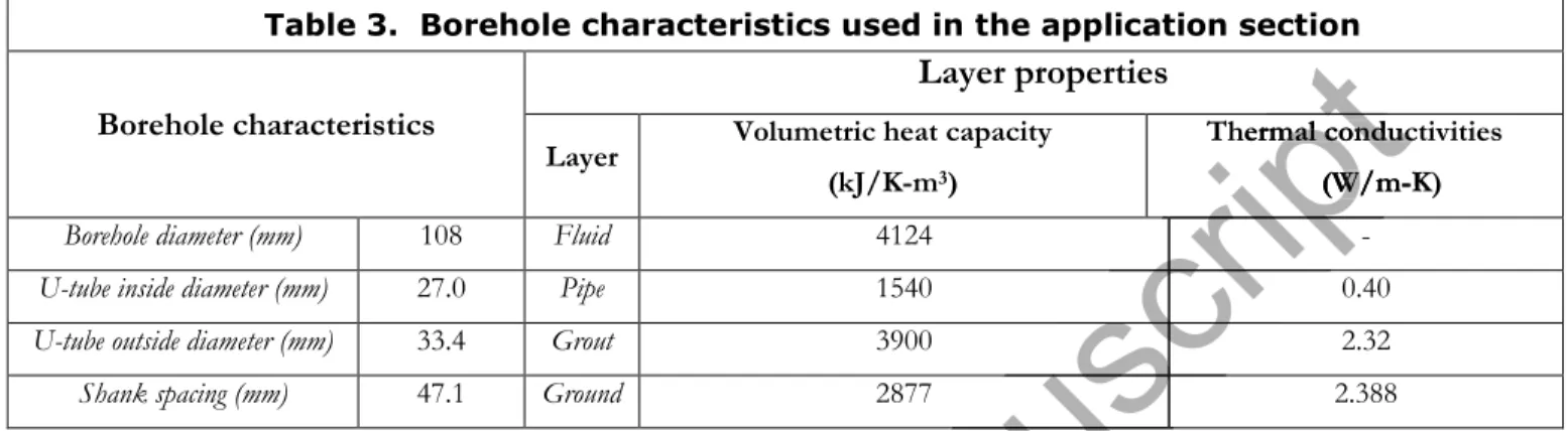
The results from the proposed model are compared with the experimental data of Beier et al. (2011). The system parameters, geometry and thermal conductivities are taken from Table 1 of Beier et al. (2011). The specific heat capacities for the fluid, pipe, grout and ground are taken as 4.2, 1.8, 3.8, and 3.2 kJ/kg-K, respectively, based on the work of Minaei and Marefat (2017a). The experimental values of inlet temperatures and flow rates are used as

Accepted Manuscript

is the internal convection coefficient. Finally, the borehole wall

Accepted Manuscript

is the internal convection coefficient. Finally, the borehole wall by the infinite cylindrical heat source solution (ICS) to ground heat transfer

Accepted Manuscript

by the infinite cylindrical heat source solution (ICS) to ground heat transfer ICS analytical solution requires the heat transfer rate at the borehole wall,

Accepted Manuscript

ICS analytical solution requires the heat transfer rate at the borehole wall, value is obtained from the numerical solution of borehole heat transfer as follows:

Accepted Manuscript

value is obtained from the numerical solution of borehole heat transfer as follows:

𝑒𝑞

Accepted Manuscript

𝑒𝑞,

Accepted Manuscript

,𝑔𝑡

Accepted Manuscript

𝑔𝑡 𝑇

Accepted Manuscript

𝑇𝑤

Accepted Manuscript

𝑤 𝑇𝑤 𝑇

Accepted Manuscript

𝑇𝑤 𝑇 −

Accepted Manuscript

− 𝑇

Accepted Manuscript

𝑇𝑤

Accepted Manuscript

𝑤 𝑇𝑤 𝑇

Accepted Manuscript

𝑇𝑤 𝑇 ,

Accepted Manuscript

,𝑠

Accepted Manuscript

𝑠 𝑙𝑛

Accepted Manuscript

𝑙𝑛 (

Accepted Manuscript

(𝑟

Accepted Manuscript

𝑟𝑏

Accepted Manuscript

𝑏 𝑟𝑏 𝑟

Accepted Manuscript

𝑟𝑏 𝑟 𝑟

Accepted Manuscript

𝑟𝑤

Accepted Manuscript

𝑤 𝑟𝑤 𝑟

Accepted Manuscript

𝑟𝑤 𝑟 ,

Accepted Manuscript

,𝑠

Accepted Manuscript

𝑠

Accepted Manuscript

)

Accepted Manuscript

)

Accepted Manuscript

refers to the node immediately upstream of the last node. In turn, the

Accepted Manuscript

refers to the node immediately upstream of the last node. In turn, the is used to obtain the borehole wall temperature using temporal superposition as follows:

Accepted Manuscript

is used to obtain the borehole wall temperature using temporal superposition as follows:

𝑇

Accepted Manuscript

𝑇𝑔

Accepted Manuscript

𝑔 𝑇𝑔 𝑇

Accepted Manuscript

𝑇𝑔 𝑇 =

Accepted Manuscript

= ∑

Accepted Manuscript

∑(

Accepted Manuscript

(𝑞

Accepted Manuscript

𝑞𝑤

Accepted Manuscript

𝑤,

Accepted Manuscript

,𝑖

Accepted Manuscript

𝑖−

Accepted Manuscript

− 𝑞

Accepted Manuscript

𝑞𝑤

Accepted Manuscript

𝑤 𝑛

Accepted Manuscript

𝑛_𝑡

Accepted Manuscript

𝑡 𝑖

Accepted Manuscript

𝑖=

Accepted Manuscript

=1

Accepted Manuscript

1

he total number of time steps,

Accepted Manuscript

he total number of time steps, 𝛤

Accepted Manuscript

𝛤 =

Accepted Manuscript

= 1

Accepted Manuscript

1 𝑘

Accepted Manuscript

𝑘𝑔

Accepted Manuscript

𝑔

Accepted Manuscript

𝐺

Accepted Manuscript

𝐺(

Accepted Manuscript

(𝐹𝑜

Accepted Manuscript

𝐹𝑜 is the solution of the ICS.

Accepted Manuscript

is the solution of the ICS. A number of

Accepted Manuscript

A number of provided by Cooper (1976) is used here.

Accepted Manuscript

provided by Cooper (1976) is used here. The proposed model has been subjected to a grid independence analysis.

Accepted Manuscript

The proposed model has been subjected to a grid independence analysis. Brussieux and Bernier

Accepted Manuscript

Brussieux and Bernier concentric cylinder, and a time step

Accepted Manuscript

concentric cylinder, and a time step

Accepted Manuscript

results from the proposed model

Accepted Manuscript

(14)

12

inputs to the proposed model. Figure 4 presents the outlet temperature as a function of time predicted by the proposed model and measured by Beier et al. (2011). There is very good agreement between the proposed model and the experiments. The maximum difference is +0.25 K and occurs at the beginning of the test where the outlet temperature experiences a steep change. When averaged for the full test duration the difference is +0.16 K.

Figure 4 Comparison between the outlet fluid temperature predicted by the proposed model and those measured by Beier et al. (2011).

Limits of the proposed model

The prediction of the outlet temperature with the proposed model relies on three major assumptions. First, it is a 1D model and only radial heat transfer is considered. Since the proposed model is used here for short operating times (less than ~ 100 hours), longitudinal heat transfer should be negligible (Philippe et al., 2009) so this assumption should not affect the results significantly. The assumption of the single pipe geometry implies that the

Accepted Manuscript

Comparison between the outlet fluid temperature predicted by the proposed model and

Accepted Manuscript

Comparison between the outlet fluid temperature predicted by the proposed model and

Limits of the proposed model

Accepted Manuscript

(15)

13

thermal short circuit between the two pipes is not considered. The impact of this assumption depends on the borehole size, the flow rate and the fluid temperature. This issue can be partly addressed using an equivalent thermal resistance, 𝑅𝑏∗ (Javed and Spitler, 2017), which accounts for the thermal short-circuit. Finally, the fluid temperature is assumed to evolve linearly between the inlet and outlet of the borehole. As will be shown shortly the use of 𝑅𝑏∗ alleviates the deficiencies of this assumption. Rees and He (2013) highlighted the existence of non-linearity in fluid temperature for short times. This non-non-linearity is mainly due to thermal capacity effects and fluid transport phenomena. In extreme cases, the model can lead to inconsistencies. For example, if the entering fluid temperature increases between two time steps but with a very small flow rate, capacity effects will be dominant, so the fluid temperature in the borehole will not change significantly. However, the model considers that the fluid temperature is the mean of the inlet and outlet temperatures. Consequently, the outlet temperature will decrease by a value equivalent to the inlet temperature increase.

To illustrate the limits imposed by these three assumptions, results from the proposed model are compared with a 2D thermal resistance and capacitance (TRCM) model (Godefroy and Bernier, 2014) for a typical borehole. The TRCM model considers the internal fluid temperature distribution as well as the thermal short circuit and it is used here with a vertical discretization of 10 segments. The ground and borehole temperatures are initially set at 0 °C and the inlet temperature is constant at 30 °C. The borehole length is fixed at 100 m and only the flow rate is varied to modify the residence time of the fluid in the borehole.

Results of this comparison are shown on Figure 5 where the outlet temperature predicted by the two approaches are given for three different fluid replacement rates for a 10-hour simulation period. The fluid replacement rate is defined here as the number of times the fluid is replaced in the entire borehole during a given time step. In other words, it is given by the time step divided by the residence time. Thus, a fluid replacement rate of 1.0 indicates that the fluid has traveled from the inlet to the outlet of the borehole during the calculation time step. Figure 5a uses the traditional borehole thermal resistance, 𝑅𝑏, based on the first order multipole while Figure 5b uses 𝑅𝑏∗ (Javed and Spitler, 2017).

Accepted Manuscript

, the model can lead to inconsistencies. For example, if the entering fluid

Accepted Manuscript

, the model can lead to inconsistencies. For example, if the entering fluid ll flow rate, capacity effects will be dominant,

Accepted Manuscript

ll flow rate, capacity effects will be dominant, . However, the model considers that the fluid

Accepted Manuscript

. However, the model considers that the fluid the outlet temp

Accepted Manuscript

the outlet temperature will decrease

Accepted Manuscript

erature will decrease results from the proposed model are compared with a

Accepted Manuscript

results from the proposed model are compared with a nd Bernier,

Accepted Manuscript

nd Bernier, 2014

Accepted Manuscript

2014)

Accepted Manuscript

)

the internal fluid temperature distribution as well as the thermal short circuit and it

Accepted Manuscript

the internal fluid temperature distribution as well as the thermal short circuit and it The ground

Accepted Manuscript

The ground and borehole

Accepted Manuscript

and borehole borehole length

Accepted Manuscript

borehole length is fixed at

Accepted Manuscript

is fixed at of the fluid in the borehole.

Accepted Manuscript

of the fluid in the borehole. Results of this comparison are shown on Figure

Accepted Manuscript

Results of this comparison are shown on Figure 5

Accepted Manuscript

5 where t

Accepted Manuscript

where the outlet temperature predicted by the two approaches

Accepted Manuscript

he outlet temperature predicted by the two approaches are given for three different fluid replacement rates

Accepted Manuscript

are given for three different fluid replacement rates for a

Accepted Manuscript

for a

Accepted Manuscript

10

Accepted Manuscript

10

defined here as the number of times the fluid is replaced in the entire borehole duri

Accepted Manuscript

defined here as the number of times the fluid is replaced in the entire borehole duri words, it is given by the time step divided by the residence time.

Accepted Manuscript

words, it is given by the time step divided by the residence time. that the fluid has traveled from the inlet to the outlet of the borehole

Accepted Manuscript

that the fluid has traveled from the inlet to the outlet of the borehole

Accepted Manuscript

uses the traditional borehole thermal resistance,

Accepted Manuscript

uses the traditional borehole thermal resistance, (Javed and Spitler, 2017).