Compensation of Tool Deflection in Robotic-Based Milling

HAL Id: hal-00700003

https://hal.archives-ouvertes.fr/hal-00700003

Submitted on 25 Jun 2019

HAL is a multi-disciplinary open access

archive for the deposit and dissemination of

sci-entific research documents, whether they are

pub-lished or not. The documents may come from

teaching and research institutions in France or

abroad, or from public or private research centers.

L’archive ouverte pluridisciplinaire HAL, est

destinée au dépôt et à la diffusion de documents

scientifiques de niveau recherche, publiés ou non,

émanant des établissements d’enseignement et de

recherche français ou étrangers, des laboratoires

publics ou privés.

Compensation of Tool Deflection in Robotic-Based

Milling

Alexandr Klimchik, Dmitry Bondarenko, Anatol Pashkevich, Sébastien Briot,

Benoît Furet

To cite this version:

Alexandr Klimchik, Dmitry Bondarenko, Anatol Pashkevich, Sébastien Briot, Benoît Furet.

Compen-sation of Tool Deflection in Robotic-Based Milling. 9th International Conference on Informatics in

Control, Automation and Robotics (ICINCO 2012), Jul 2012, Rome, Italy. �hal-00700003�

COMPENSATION OF TOOL DEFLECTION

IN ROBOTIC-BASED MILLING

Alexandr Klimchik

1,2

, Dmitry Bondarenko

2,3

, Anatol Pashkevich

1,2

, Sebastien Briot

2

, Benôit Furet

2,4 1

Ecole des Mines de Nantes, 4 rue Alfred-Kastler, 44307 Nantes, France

2

Institut de Recherches en Communications et Cybernétique de Nantes, UMR CNRS 6597, France

3

Ecole Centrale de Nantes, 1 rue de la Noë, 44 321 Nantes, France

3

Université de Nantes, quai de Tourville, 44035 Nantes, France {alexandr.klimchik, anatol.pashkevich}@mines-nantes.fr, {dmitry.bondarenko, sebastien.briot, benoit.furet}@irccyn.ec-nantes.fr

Keywords: Industrial robot, milling, compliance error compensation, dynamic machining force model, non-linear stiff-ness model.

Abstract: The paper presents the compliance errors compensation technique for industrial robots, which are used in milling manufacturing cells. under external loading, which is based on the non-linear stiffness model. In contrast to previous works, it takes into account the interaction between the milling tool and the workpiece that depends on the end-effector position, process parameters and cutting conditions (spindle rotation, feed rate, geometry of the tool, etc.). Within the developed technique, the compensation errors caused by external loading is based on the non-linear stiffness model and reduces to a proper adjusting of a target trajectory that is modified in the off-line mode. The advantages and practical significance of the proposed technique are illustrated by an example that deals with milling with Kuka robot.

1 INTRODUCTION

Currently, robots become more and more popular for a variety of technological processes, including high-speed precision machining. For this process, the robot is subjected by external loading which caused by the machining force. This force is gener-ated by the interaction between the tool mounted on the robot end-effector and the workpiece during the material removal (Dépincé, 2006). It is a contact force and it is distributed along the affected area of the tool cutting part. To evaluate the influence and to analyze the robot behavior while machining, the cut-ting force should be defined either experimentally or using accurate mathematical model.

To evaluate the force caused by interaction be-tween the tool and the workpiece, two approaches can be used. The static approach allows computing the average cutting force without any consideration of dynamic aspect in machining system. This force serves as an external loading of the robot. This ap-proach is widely used in analysis of conventional machining processes using CNC machines (Altintas,

2000), where the stiffness is high. In contrast, robots have relatively low structural stiffness. For this rea-son, in the case of robotic-based machining, an addi-tional source of dynamic displacements of the end-effector with respect to the desired trajectory in-duced by robot compliance may arise. Such behavior leads to the variable contact between the machining tool and the workpiece. Thus, the generated contact force depends on the current position of the robot end-effector on the trajectory. Consequently, the cutting force cannot be evaluated correctly using the static approach. In this case, the dynamic approach, which will be used in the paper, is required. It is based on computing of the force at each instant of machining process that defines loading of the robot for the next instant of processing. As a result, the dynamic aspect of robot motion under such variable cutting force can be examined for whole process.

Usually, in the robot-based machining this force causes essential deflections that decrease the quality of the final product. The problem of the robot error compensation can be solved in two ways that differ in degree of modification of the robot control soft-ware:

(a) by modification of the manipulator model, which better suits to the real manipulator and is used by the robot controller (in simple case, it can be lim-ited by tuning of the nominal manipulator model, but may also involve essential model enhancement by introducing additional parameters, if it is allowed by a robot manufacturer);

(b) by modification of the robot control program that defines the prescribed trajectory in Cartesian space (here, using relevant error model, the input trajectory is generated in such way that under the loading the output trajectory coincides with the de-sired one, while input trajectory differs from the tar-get one).

Moreover, with regard to the robot-based ma-chining, there is a solution that does not require force/torque measurements or computations (Dé-pincé, 2006), where the target trajectory for the ro-bot controller is modified by applying the "mirror" technique. An evident advantage of this technique is its applicability to the compensation of all types of the robot errors, including geometrical and compli-ance ones. However, this approach requires carrying out additional preliminary experiments which are quite expensive. So, it is suitable for the large-scale production only. Another compensation methodolo-gy has been proposed by Eastwood and Webb (Eastwood, 2010) that was used for gravitational de-flection compensation for hybrid parallel kinematic machines.

This paper focuses on the modification of control program that is considered to be more realistic in practice. This approach requires also accurate stiff-ness model of the manipulator. From point of view of stiffness analysis, the external and forces directly influence on the manipulator equilibrium configura-tion and, accordingly, may modify the stiffness properties. So, they must be undoubtedly taken into account while developing the stiffness model. How-ever, in most of the related works the Cartesian stiffness matrix has been computed for the nominal configuration (Chen, 2000; Alici, 2005). Such ap-proach is suitable for the case of small deflections only. For the opposite case, the most important re-sults have been obtained in (Kövecses, 2007; Tyapin, 2009; Pashkevich, 2011), which deal with the stiffness analysis of manipulators under the end-point loading.

Thus, to compensate errors caused by the ma-chining process, it is required to have an accurate stiffness model and precise cutting force model. In contrast to the previous works, the compliance error compensation technique presented in this work is based on the non-linear stiffness model of the ma-nipulator (Pashkevich, 2011) and dynamic model of technological process that generates the cutting force.

2 PROBLEM STATEMENT

For the compliance errors, the compensation technique must rely on two components. The first of them describes distribution of the stiffness properties throughout the workspace and is defined by the stiffness matrix as a function of the joint coordi-nates. The second component describes the forc-es/torques acting on the end-effector while the ma-nipulator is performing its machining task (manipu-lator loading).

The stiffness matrix required for the compliance errors compensation highly depends on the robot configuration and essentially varies throughout the workspace. From general point of view, full-scale compensation of the compliance errors requires es-sential revision of the manipulator model embedded in the robot controller. In fact, instead of conven-tional geometrical model that provides inverse/direct coordinate transformations from the joint to Carte-sian spaces and vice versa, here it is necessary to employ the so-called kinetostatic model (Su, 2006). It is essentially more complicated than the geometri-cal model and requires rather intensive computations that are presented in Section 3..

The dynamic behavior of the robot under the loading F caused by technological process can be described as

C  C  C 

M δt C δt K δt F (1)

where M is _C 6 6 mass matrix that represents the global behavior of the robot in terms of natural fre-quencies, C_C is 6 6 damping matrix, K_C is 6 6 Cartesian stiffness matrix of the robot under the ex-ternal loading F, δt δt and δt are dynamic dis-, placement, velocity and acceleration of the tool end-point in a current moment respectively (Briot, 2011).

In general, the cutting force Fc has a nonlinear

nature and depends on many factors such as cutting conditions, properties of workpiece material and tool cutting part, etc (Ritou, 2006). But, for given tool/workpiece combination, the force Fc could be

approximated as a function of an uncut chip thick-ness h, which represents the desired thickthick-ness to cut at each instant of machining.

Hence, to reduce errors caused by cutting forces in the robotic-based machining it is required to ob-tain an accurate elasto-static model of robot and elasto-dynamic model of machining process. These problems are addressed in the following sections taking into account some particularities of the con-sidered application (robotic-based milling).

3 MANIPULATOR MODEL

3.1 Elasto-static model

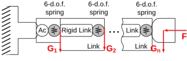
Elasto-static model of a serial robot is usually de-fined by its Cartesian stiffness matrix, which should be computed in the neighborhood of loaded configu-ration. Let us propose numerical technique for com-puting static equilibrium configuration for a general type of serial manipulator. Such manipulator may be approximated as a set of rigid links and virtual joints, which take into account elasto-static proper-ties (Figure 1). Since the link weight of serial robots is not negligible, it is reasonable to decompose it into two parts (based on the link mass centre) and apply them to the both ends of the link. All this load-ings will be aggregated in a vector G



G₁...Gn



,

where G_i is the loading applied to the i-th node-point. Besides, it is assumed that the external load-ing F (caused by the interaction of the tool and the workpiece) is applied to the robot end-effector.

...

Link

Ac Rigid Link Link Link 6-d.o.f. spring 6-d.o.f. spring 6-d.o.f. spring F Gn G2 G1

Figure 1 VJM model of industrial robot with end-point and auxiliary loading

Following the principle of virtual work, the work of external forces G F is equal to the work of in-, ternal forces τ_ caused by displacement of the vir-tual springs δθ



T



T T θ 1 δ δ δ n j j j     



G t F t τ θ (2)

where the virtual displacements δt can be com-_j

puted from the linearized geometrical model derived from ( )

θ

δ jδ , 1..

j j n

t J θ , which includes the Jaco-bian matrices _θ( )j

 

,

j

  

J g q θ θ with respect to the virtual joint coordinates.

So, expression (2) can be rewritten as



T ( )

 

T ( )



T θ θ θ 1 δ δ δ n j n j j       



G J θ F J θ τ θ (3)

which has to be satisfied for any variation of δθ . It means that the terms regrouping the variables δθ have the coefficients equal to zero. Hence the force balance equations can be written as

( )T ( )T θ θ θ 1 n j n j j 



   τ J G J F (4)

These equations can be re-written in block-matrix form as (G)T (F)T θ  θ   θ  τ J G J F (5) where (F) ( ) θ θ n  J J , (G) (1) ( ) θ θ θ T T_... nT      J J J , T T T 1 ... n     

G G G . Finally, taking into account the virtual spring reaction τ_θ K θ_θ , where



1 n



θ diag θ,..., θ

K K K , the desired static equilib-rium equations can be presented as

(G)T (F)T

θ   θ   θ

J G J F K θ (6)

To obtain a relation between the external loading F and internal coordinates of the kinematic chain θ corresponding to the static equilibrium, equations (6) should be solved either for different given values of F or for different given values of t. Let us solve the static equilibrium equations with respect to the manipulator configuration θ and the external load-ing F for given end-effector position tg θ

 

and the function of auxiliary-loadings G θ

 

 

 

(G)T (F)T

θ  θ  θ ;  ; 

K θ J G J F t g θ G G θ (7) where the unknown variables are



θ F,



.

Since usually this system has no analytical solu-tion, iterative numerical technique can be applied. So, the kinematic equations may be linearized in the neighborhood of the current configuration θ_i

 

(F)

  



θ

1 1 ;

i  i  i  i  i

t g θ J θ θ θ (8)

where the subscript 'i' indicates the iteration number and the changes in Jacobians (G) (F)

θ , θ

J J and the auxil-iary loadings G are assumed to be negligible from iteration to iteration. Correspondingly, the static equilibrium equations in the neighborhood of θ_i may be rewritten as

(G)T (F)T

θ   θ  i1 θ i1

J G J F K θ . (9)

Thus, combining (8), (9) and analytical expres-sion for 1 (G)T (F)T

θ ( θ θ )



   

θ K J G J F , the unknown

variables F and θcan be computed using follow-ing iterative scheme





 









1 (F) 1 (F)T θ θ (F) (F) 1 (G)T θ θ θ 1 (G)T (F)T θ θ 1 1 1 θ 1 · i i i i i i i i                     F J K J t g θ J θ J K J G θ K J G J F (10)

The proposed algorithm allows us to compute the static equilibrium configuration for the serial robot under external loadings applied to any point of the manipulator and the loading from the technological process.

3.2 Stiffness matrix

In order to obtain the Cartesian stiffness matrix, let us linearize the force-deflection relation in the neighborhood of the equilibrium. Following this ap-proach, two equilibriums that correspond to the ma-nipulator state variables ( , , )F θ t and

(Fδ ,F θδ ,θ tδ )t should be considered simul-taneously. Here, notations δF , δt define small in-crements of the external loading and relevant dis-placement of the end-point. Finally, the static equi-librium equations may be written as

 

(G)T (F)T θ θ θ ;       t g θ K θ J G J F (11) and

























T (G) (G) θ θ θ T (F) (F) θ θ δ δ δ δ δ δ δ              t t g θ θ K θ θ J J G G J J F F (12)

where t F G K θ, , , _θ, are assumed to be known. After linearization of the function g θ( ) in the neighborhood of the loaded equilibrium, the system (11), (12) is reduced to equations (F) θ (G) (G) (F) (F) θ θ θ θ θ δ δ δ δ δ δ δ       t J θ K θ J G J G J F J F (13)

which defines the desired linear relations between δt and δF . In this system, small variations of Jaco-bians may be expressed via the second order deriva-tives (F) (F) θ θθ δJ H δθ , (G) (G) θ θθ δJ H δθ , where (G) 2 θθ 1 2 T j j j n  



  H g G θ , (F θθ)  2 T  2 H g F θ .

Also, the auxiliary loading G may be computed via the first order derivatives as δG   G θ δθ

Further, let us introduce additional notation

(F) (G) (G)T

θθ θθ  θθ  θ  

H H H J G θ , which allows us

to present system (13) in the form

(F) θ (F)T θ θ θθ δ δ δ    _{ }      _{ }         0 J t F 0 J K H θ (14)

So, the desired Cartesian stiffness matrices K_C can be computed as



_{(F) 1 (F)T}



1 C θ ( θ θθ) θ     K J K H J (15)

Below, this expression will be used for compu-ting of the elasto-static deflections of the robotic manipulator.

3.3 Mass matrix

To evaluate dynamic behaviour of the robot under the loading, in addition to the Cartesian stiffness ma-trix K_C it is required to define the mass matrix M . _C

Comprehensive analysis and definition of this matrix have been proposed in (Briot, 2011). Here, let us summarise the main results that will be used further in the error compensation technique.

Similar to the stiffness matrix, here physical properties defined by the mass matrix M are con-_C

stant in the joint coordinates M_θ const and are defined by the mass matrices M of all _θi n links of the robot M_θ diag(M_θ1,...,M_θn). Assuming that link may be approximated by a beam with a constant cross-section, the mass matrix M can be computed _θi

as θidiag a a( ,1 2,a3,a4,a5,a6) M (16) where a₁m_i/ 3, a₂33m_i/ 140, a₃33m_i/ 140, 4 / 3 p i i i a I L , a₅8I_iy_iL_i/ 15, a₆8I_iz_iL_i/ 15, i

m is physical mass of i-th link, _i is density of i-th link, L_i is link length, p

i

I is the polar moment, ,

y z i i

I I are the second moments of the area. Since the mass matrix M_θ is defined in the joint coordinates it can be recomputed into the Cartesian coordinates associated with the tool end-point using the Jacobian matrix J_θ (which depend on the robot configuration q and computed with respect to virtual joint coordi-nates θ) using following expression

θ

C θ θ

T



M J M J (17)

Thus, using expressions (16) and (17) it is possi-ble to compute the mass matrix M for a given ro-_C

bot configuration q.

4 MACHINING PROCESS

Let us obtain the model of the cutting force which depends on the relative position of the tool with respect to the workpiece at each instant of ma-chining. As follows from previous works (Brissaud, 2008), for the known chip thickness h, the cutting force Fc can be expresses as

 

0





2 , 0 1 s s c s p h h r h h F h k a h h h     (18)

where a_p is a depth of cut, rk_ k₀1 depends on the parameters k∞, k0 that define the so called stiffness of the cutting process for large and small chip thickness h respectively (Figure 2) and hs is a specific chip thickness, which depends on the cur-rent state of the tool cutting edge. The parameters k0,

hs, r are evaluated experimentally for a given com-bination of tool/working material. To take into ac-count the possible loss of contact between the tool and the workpiece, expression (18) should be sup-plement by the case of h0 as

h

s

~k

∞

~k

0

F

c

h

Range of h in case of conventional CNC machining

Figure 2 Fractional cutting force model Fc(h)

 

0, if 0

c

F h  h (19)

For the multi-edge tool the machining surface is formed by means of several edges simultaneously. The number of working edges varies during machin-ing and depends on the width of cut. For this reason, the total force Fc of such interaction is a

superposi-tion of forces Fc,i generated by each tool edge i,

which are currently in the contact with the workpiece. Besides, the contact force Fc,i can be

de-composed by its radial Fr,i and tangential Ft,i

com-ponents (Figure 3). In accordance with Merchant’s model (Merchant, 1945), the t-component of cutting force Ft,i can be computed with the equation (18).

The r-component Fr,i is related with Ft,i by following

expression (Laporte 2009)

, ,

r i r t i

F k F (20)

where the ratio factor kr depends on the given

tool/workpiece characteristics.

It should be mentioned that in robotic machining it is more suitable to operate with forces expressed in the robot tool frame {x,y,z}. Then, the corre-sponding components Fx, Fy (Figure 3) of the cutting

force Fc can be expressed as follows

, , 1 1 , , 1 1 cos sin sin cos z z z z n n x r i i t i i i i n n y r i i t i i i i F F F F F F             









(21)

where nz is the number of currently working cutting

edges, φi is the angular position of the i-th cutting

edge (the cutting force in z direction Fz is negligible

here). So, the vector of external loading of the robot

due to the machining process can be composed in the frame {x,y,z} using the defined components Fx, Fy as F=[Fx,Fy,0,0,0,0]T. i i Fr,i Ft,i Fx Fy vf W TCP Workpiece Cutter y x Cutting direction

Figure 3 Forces of tool/workpiece interaction

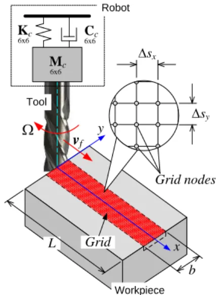
vf W Cc 6x6 Dsy Dsx Grid nodes Grid _x y L b Mc 6x6 Kc 6x6 Robot Tool Workpiece

Figure 4 Meshing of the workpiece area

It should be stressed that the cutting force com-ponents Fr,i, Ft,i mentioned in equation (18),(20) are

computed for the given chip thickness hi, which

should be also evaluated. Let us define model for hi

using mechanical approach. Then the chip thickness hi removed by i-th tooth depends on the angular

po-sition φi of this tooth and it can be evaluated using to

the geometrical distance between the position of the given tooth i and the current machining profile (Figure 3). It should be mentioned, that the main is-sue here is to follow the current relative position be-tween the i-th tooth and the working material or to define whether the i-th tooth is involved in cutting for given instant of process. Because of the robot dynamic behavior and the regenerative mechanism of surface formation (Tlusty, 1981) this problem cannot be solved directly using kinematic relations.

In this case it is reasonable to introduce a special rectangular grid, which decomposes the workpiece area into segments and allows tracking the tool/workpiece interaction and the formation of the machining profile (Figure 4).

Here, Steps Δsx, Δsy between grid nodes are

stant and depend on the tool geometry, cutting con-dition and time discretization Δτ. Each node j (j1,N_w, Nw is the number of nodes) of the grid

can be marked as “1” or “0”: “1” corresponds to nodes situated in the workpiece area with material (rose nodes in Figure 5), “0” corresponds to nodes situated in workpiece area that was cut away (white nodes in Figure 5).

In order to define the number of currently cut nodes by the i-th tooth, the previous instant of ma-chining process should be considered. Let us define Ai as an amount of working material that is currently

cut away by the i-th tooth (Figure 5). So, if node j marked as “1” is located inside the marked sector (green nodes in Figure 5), it changes to “0” and Ai is

increasing by D Ds_x s_y. Analyzing all potential nodes and computing Ai, the chip thickness hi, removed at

given instant of the process by the i-th tooth, can be estimated by h_iA R_i D_i, i1,Nz. The angle

Δφi determines the current angular position of the

i-th tooi-th regarding to its position at i-the instant τ-Δτ and referred to the position of TCP at τ-Δτ.

W

D

v

f Workpiece TCPτ Grid nodes Removing material Ai TCPτ-Dτ x y

Figure 5 Evaluating the tool/workpiece intersection Ai

and computing the corresponding chip thickness hi

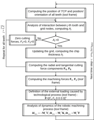
Described mechanism of chip formation and the machining force model (18) allow computing the dynamic behavior of the robotic machining process where models of robot inertia and stiffness are dis-cussed in the section 3 of the paper. The detailed al-gorithm that is used in numerical analysis is present-ed in Figure 6, where the analysis of the robot dy-namics is performed in the tool frame with respect to the dynamic displacement of the tool δtdyn fixed on

the robot end-effector around its position on the tra-jectory..

Computing the position of TCP and position/ orientation of all teeth (tool frame)

Analysis of interaction between j-th tooth and

grid nodes, computing Aj

Updating the grid, computing the chip

thickness hj

Definition of the external loading caused by technological process (tool frame) :

F=[Fx Fy 0 0 0 0]T Aj >0 R e p e a t fo r a ll te e th Yes No Zero cutting forces, Frj=0, Ftj=0

Computing the radial and tangential cutting

force components Frj, Ftj

Computing the machining forces Fx, Fy (tool

frame)

Analysis of dynamics of the robotic machining process (tool frame)

N e x t ti m e s te p τ : τ = τ0 : D τ: τMA X Z j ,1  1 1 1

dyn c c dyn c c dyn c

  

   

δt M C δt M K δt M F

Figure 6 Algorithm for numerical simulation of robotic machining process dynamics

5 COMPLIANCE ERROR

COMPENSATION TECHNIQUE

In industrial robotic controllers, the manipulator mo-tions are usually generated using the inverse kine-matic model that allows us to compute the input sig-nals for actuators ρ₀ corresponding to the desired end-effector location t₀, which is assigned assum-ing that the compliance errors are negligible. How-ever, if the external loading F is essential, the ki-nematic control becomes non-applicable because of changes in the end-effector location. It can be com-puted from the non-linear compliance model as





1 F f | 0   t F t (22)

where the subscripts 'F' and '0' refer to the loaded and unloaded modes respectively, and '|' separates arguments and parameters of the function f

 

. Some details concerning this function are given in our previous publication (Pashkevich, 2011).

To compensate this undeterred end-effector dis-placement from t₀ to t_F, the target point should be modified in such a way that, under the loading F,

the end-platform is located in the desired point t₀. This requirement can be expressed using the stiff-ness model in the following way



(F)



0| 0 f  F t t (23) where (F) 0

t denotes the modified target location. Hence, the problem is reduced to the solution of the nonlinear equation (23) for (F)

0

t , while F and t₀ are assumed to be given. It is worth mentioning that this equation completely differs from the equation

0

( | )

f 

F t t , where the unknown variable is t. It means that here the compliance model does not al-low us to compute the modified target point (F)

0

t

straightforwardly, while the linear compensation technique directly operates with Cartesian compli-ance matrix (Gong, 2000).

To solve equation (23) for t(F)₀ , similar numerical technique can be applied. It yields the following it-erative scheme





(F) (F) 1 (F) 0 0 · 0 f ( | 0 )      t t t F t (24)

where the prime corresponds to the next iteration, (0,1)

  is the scalar parameter ensuring the con-vergence. More detailed presentation of the devel-oped iterative routines is given in Figure 7.

  F t ) F ( 1 0 | ε f  F t  t Compute end-platform location

No Yes   1 (F) 0 | f  F t F t N e x t it e ra ti o n     0 j  ;  ( )j t t F 0 F F t Obtain trajectory t



tj F t j



R e p e a t fo r d if fe re n t t0   0 j  tt Stopping criterion is satisfied?   (F) (F) 0 0  0 F t t t t 0 (F) 0  t t

Compute corresponding equilibrium configuration and stiffness matrix

( ) C , , , i i i i q θ F K

Figure 7 Procedure for compensation of compliance errors

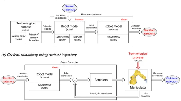
Hence, using the proposed computational tech-niques, it is possible to compensate a main part compliance errors by proper adjusting the reference trajectory that is used as an input for robotic control-ler. In this case, the control is based on the inverse kinetostatic model (instead of kinematic one) that takes into account both the manipulator geometry and elastic properties of its links and joints. Imple-mentation of developed compliance error compensa-tion technique presented in Figure 8.

(a) Off-line: modification of the target trajectory

(b) On-line: machining using revised trajectory

Modified trajectory Actuators Manipulator -Cartesian coordinates Joint encoders Joint coordinates Cartesian coordinates Robot Controller

Actual joint coordinates

Obtained trajectory Geometrical model Robot model (nominal) direct Geometrical model Stiffness model

Robot model (actual) Estimated loading Geometrical model Robot model (nominal) Error compensator Joint coordinates Desired trajectory inverse Cartesian coordinates Modified trajectory direct Cartesian coordinates Cutting force model Model of surface formation Technological process (actual) Technological process (actual)

6 EXPERIMENTAL

VERIFICATION

The developed compliance error compensation technique has been verified experimentally for ro-botic milling with the KUKA KR270 robot along a simple trajectory in aluminum workpiece. It is as-sumed that at the beginning of the technological process the robot is in the configuration q (see Ta-ble 1 Figure 9). The parameters of the stiffness mod-el for the considered robot have been identified in (Dumas, 2011) and are presented in Table 1. Link masses required for the mass matrix of the robot are presented also in Table 1.

Table 1 Initial data for robotic-based milling Joint coordinates, [deg]

q1 q2 q3 q4 q5 q6

90 -50 120 180 25 180 Joint compliances, [rad/N m]*10-6

k1 k2 k3 k4 k5 k6 0.26 0.15 0.26 1.79 1.52 2.13 Link masses, [kg] m1 m2 m3 m4 m5 m6 336.8 259.4 85.2 54.5 36.3 18.2 x y z Feed direction Workpiece

Figure 9 Starting pose of the KUKA KR270 robot to perform the operation of milling

For the milling, the cutter with the external di-ameter D=20 mm and four teeth (Nz=4) distributed

uniformly over the tool is used. For the given com-bination of the tool and the workpiece material the following parameters correspond to the cutting force model defined in (18): k0= 6 5 10 _N/m, hs=1.8 105   _{m, r=0.1, k}r=0.3.

v

f

W

Workpiece Cutter

D/2

D

Cutting direction

Figure 10 Starting relative position of the tool with respect to the workpiece

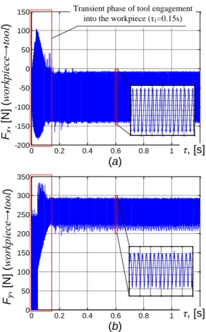
0 0.2 0.4 0.6 0.8 1 1.2 0 50 100 150 200 250 300 350 0 0.2 0.4 0.6 0.8 1 1.2 -200 -150 -100 -50 0 50 100 150 Fx , [N ] (w or kp ie ce → to ol ) τ, [s] Transient phase of tool engagement

into the workpiece (τ1=0.15s)

(a) Fy , [N ] (w or kp ie ce → to ol ) τ, [s] (b) 1 1.005 1.01 1.015 1.02 1.025 1.03 -110 -100 -90 -80 -70 -60 -50 -40 -30 -20 -10 1 1.005 1.01 1.015 1.02 1.025 1.03 170 180 190 200 210 220 230 240

Figure 11 Variation of machining force components Fx

(a) and Fy (b) for whole milling process

Taking into account that the workpiece has a straight borders let us assume that at the instant t=0 one of the teeth of the tool is in contact with the workpiece material as it is shown in the Figure 10. It is also assumed that the machining process is per-forming with the constant feed rate vf=4 m/min

(ap-plied in x-direction of the robot tool frame) and the constant spindle rotation Ω=8000 rpm along the straight line of 80 mm. Experimental verification

and numerical simulation of the described case of the milling process with KUKA KR-270 robot using the algorithm shown in Figure 6 allows us to trace the evolution of machining force x,y-components for the whole process (Figure 11). The corresponding dynamic displacement of the tool around its current position on the trajectory is shown in Figure 12.

0 0.2 0.4 0.6 0.8 1 1.2 -0.04 -0.02 0 0.02 0.04 0.06 0.08 xTCP yTCP δtd y n , [m m ] τ, [s]

Figure 12 Evolution of the tool dynamic displacement

δtdyn that is composed from xTCP and yTCP components

0 0.2 0.4 0.6 0.8 1 1.2 -5 0 5 x 10-5 0 0.2 0.4 0.6 0.8 1 1.2 -4 -2 0 x 10-5 fy , yTC P , [m m ] 10-2 vfy , [m /s ] τ, [s] τ, [s] yTCP Referenced points

Modified trajectory in y-direction

Referenced points

Modified feed rate in y-direction

Figure 13 Modified trajectory fy and corresponding feed

rate vfy in y-direction, computed based on the original

dynamic displacement of the tool δtdyn

In accordance with the obtained results the sys-tem robot/machining process realize complex vibra-tory motion. The high frequency component of this motion (about 700 Hz, Figure 11) is related to the spindle rotation and the number of tool teeth Nz. In

certain cases such behavior can excites the dynamics of the robot (natural modes) but this study remains out the frame of the presented paper. On the contra-ry, the low frequency component of robot/tool mo-tion (about 7 Hz, Figure 12), especially in the

y-direction (that is perpendicular to the applied feed) influences directly the quality of final product. Such motion is related to the robot compliance and it can be compensated using the error compensation tech-nique described in the paper. Hence, let us form the modified trajectory based on the dynamic displace-ment of the robot end-effector in the y-direction (Figure 13):

It should be stressed that the time step between referenced points of this modified trajectory is lim-ited with the characteristics of the controller used in the robot (in the presented case this step is chosen 0.05 sec). The corresponding feed rate vfy for the

modified trajectory has been computed. So, this new data (feed fy and feed rate vfy) with the data defined

in the beginning of this section allow us to compen-sate the trajectory error during machining caused by the robot compliance. The resulted compensated tra-jectory in the y-direction (in time domain) is pre-sented in Figure 14. 0 0.2 0.4 0.6 0.8 1 1.2 -0.02 -0.01 0 0.01 0.02 yT C P a ft e r c o m p e n s a ti o n , [m m ] τ, [s] Transient phase of tool engagement

into the workpiece (τ1=0.15s)

Figure 14 Evolution of the dynamic displacement obtained after involving the error compensation technique

into the analysis of robotic milling process

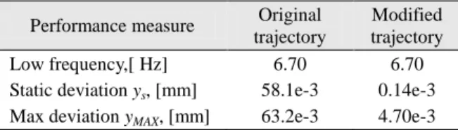
It should be noted that the part of the trajectory while machining tool is engaging into the workpiece does not have effect on the quality of final product (surface). During this stage the contact area between the tool and the workpiece is increasing progressive-ly. Hence, at each instant of processing the cutter corrects the machining profile and eliminates trajec-tory errors produced during all previous instants. On the contrary, during the stage of machining with the fully engaged tool the trajectory in x,y-directions define directly the final machining profile and this part of trajectory is analyzed here (Figure 14). Com-parison results presented in Figure 12 and Figure 14 are summarized in Table 2. So after applying error compensation technique the static deviation in y di-rection has been reduced from 0.058 mm to 0.00014 mm (99.8%). Maximum defilation in the

machining profile has been reduced from 0.063 mm to 0.0047 mm (92.6%). Low frequency remained the same for both cases.

Table 2 Milling trajectory accuracy before and after compliance error compensation

Performance measure Original trajectory

Modified trajectory Low frequency,[ Hz] 6.70 6.70 Static deviation ys, [mm] 58.1e-3 0.14e-3

Max deviation yMAX, [mm] 63.2e-3 4.70e-3

Hence, obtained results show that the developed compliance error compensation allows us signifi-cantly increase the accuracy of the robotic-based machining.

7 CONCLUSION

In robotic-based machining, an interaction be-tween the workpiece and technological tool causes essential deflections that significantly decrease the manufacturing accuracy. Relevant compliance errors highly depend on the manipulator configuration and essentially differ throughout the workspace. Their influence is especially important for heavy serial ro-bots. To overcome this difficulty this paper presents a new technique for compensation of the compliance errors caused by technological process. In contrast to previous works, this technique is based on the non-linear stiffness model and the reduced elasto-dynamic model of the robotic based milling process. The advantages and practical significance of the proposed approach are illustrated by milling with of KUKA KR270. It is shown that after error compen-sation technique significantly increase the accuracy of milling. In future the proposed technique will be integrated in a software toolbox.

ACKNOWLEDGEMENTS

The authors would like to acknowledge the fi-nancial support of the ANR, France (Project ANR-2010-SEGI-003-02-COROUSSO) and the Region “Pays de la Loire”, France.

REFERENCES

Alici G., Shirinzadeh B., 2005. Enhanced stiffness model-ing, identification and characterization for robot ma-nipulators. Proceedings of IEEE Transactions on

Ro-botics, vol. 21, pp. 554–564.

Altintas Y., 2000. Manufacturing automation, metal cut-ting mechanics, machine tool vibrations and CNC de-sign. Cambridge University Press, New York.

Brissaud D., Gouskov A., Paris H., Tichkiewitch S., 2008. The Fractional Model for the Determination of the Cutting Forces. Asian Int. J. of Science and

Technol-ogy - Production and Manufacturing, vol. 1, pp.17-25.

Briot S., Pashkevich A., Chablat D. Reduced elastody-namic modelling of parallel robots for the computation of their natural frequencies. 13th World Congress in Mechanism and Machine Science, 19 - 25 Juin, 2011, Guanajuato, Mexico.

Chen S., Kao I., 2000. Conservative Congruence Trans-formation for Joint and Cartesian Stiffness Matrices of Robotic Hands and Fingers. The International Journal

of Robotics Research, vol. 19(9), pp. 835–847.

Dépincé P., Hascoët J-Y., 2006. Active integration of tool deflection effects in end milling. Part 2. Compensation of tool deflection, International Journal of Machine

Tools and Manufacture, vol. 46, pp. 945-956

Dumas C., Caro S., Garnier S., Furet B., 2011. Joint stiff-ness identification of six-revolute industrial serial ro-bots, Robotics and Computer-Integrated

Manufactur-ing, vol. 27(4), pp. 881-888.

Eastwood S.J., Webb P., 2010. A gravitational deflection compensation strategy for HPKMs, Robotics and

Computer-Integrated Manufacturing, vol. 26 pp. 694–

702

Gong, C., Yuan J., Ni, J., 2000. Nongeometric error identi-fication and compensation for robotic system by in-verse calibration. International Journal of Machine

Tools & Manufacture, vol. 40(14) pp. 2119–2137.

Kövecses J., AngelesJ., 2007. The stiffness matrix in elas-tically articulated rigid-body systems. Multibody

Sys-tem Dynamics. vol. 18(2), pp. 169–184.

Laporte S., K’nevez J.-Y., Cahuc O., Darnis P., 2009. Phenomenological model for drilling operation. Int. J.

of Advanced Manufacturing Technology, vol.40,

pp.1-11.

Merchant M.E., 1945. Mechanics of metal cutting process. I-Orthogonal cutting and type 2 chip. Journal of

Ap-plied Physics, vol.16(5), pp.267–275.

Pashkevich A., Klimchik A., Chablat D., 2011. Enhanced stiffness modeling of manipulators with passive joints.

Mech. and Machine Theory, vol. 46(5), pp. 662-679.

Ritou M., Garnier S., Furet B., Hascoet J.Y., 2006. A new versatile in-process monitoring system for milling, Int.

J. of Machine Tools & Manufacture, 46/15:2026-2035.

Tlusty J., Ismail F., 1981, Basic non-linearity in machin-ing chatter. Annals of CIRP, Vol.30/1, pp.299-304. Tyapin I., Hovland G., 2009. Kinematic and elastostatic

design optimization of the 3-DOF Gantry-Tau parallel kinamatic manipulator. Modelling, Identification and

Control, vol. 30(2), pp. 39-56

Su H.-J., McCarthy J.M., 2006. A Polynomial Homotopy Formulation of the Inverse Static Analyses of Planar Compliant Mechanisms. Journal of Mechanical