HAL Id: hal-00661725
https://hal.archives-ouvertes.fr/hal-00661725
Submitted on 20 Jan 2012
HAL is a multi-disciplinary open access
archive for the deposit and dissemination of sci-entific research documents, whether they are pub-lished or not. The documents may come from
L’archive ouverte pluridisciplinaire HAL, est destinée au dépôt et à la diffusion de documents scientifiques de niveau recherche, publiés ou non, émanant des établissements d’enseignement et de
Shape analysis of local facial patches for 3D facial
expression recognition
Ahmed Maalej, Boulbaba Ben Amor, Mohamed Daoudi, Anuj Srivastava,
Stefano Berretti
To cite this version:
Ahmed Maalej, Boulbaba Ben Amor, Mohamed Daoudi, Anuj Srivastava, Stefano Berretti. Shape analysis of local facial patches for 3D facial expression recognition. Pattern Recognition, Elsevier, 2011, 44 (8), pp.1581-1589. �10.1016/j.patcog.2011.02.012�. �hal-00661725�
Shape Analysis of Local Facial Patches for 3D Facial
Expression Recognition
Ahmed Maaleja,b, Boulbaba Ben Amora,b, Mohamed Daoudia,b,
Anuj Srivastavac, Stefano Berrettid,
a
LIFL (UMR CNRS 8022), University of Lille1, France. b
Institut TELECOM ; TELECOM Lille 1, France. c
Department of Statistics, Florida State University, USA. d
Dipartimento di Sistemi e Informatica, University of Firenze, Italy.
Abstract
In this paper we address the problem of 3D facial expression recognition. We propose a local geometric shape analysis of facial surfaces coupled with ma-chine learning techniques for expression classification. A computation of the length of the geodesic path between corresponding patches, using a Rieman-nian framework, in a shape space provides a quantitative information about their similarities. These measures are then used as inputs to several classi-fication methods. The experimental results demonstrate the effectiveness of the proposed approach. Using Multi-boosting and Support Vector Machines (SVM) classifiers, we achieved 98.81% and 97.75% recognition average rates, respectively, for recognition of the six prototypical facial expressions on BU-3DFE database. A comparative study using the same experimental setting shows that the suggested approach outperforms previous work.
Keywords: 3D facial expression classification, shape analysis, geodesic path, multi-boosting, SVM.
1. Introduction
1
In recent years, 3D facial expression recognition has received growing
2
attention. It has become an active research topic in computer vision and
3
pattern recognition community, impacting important applications in fields
4
related to human-machine interaction (e.g., interactive computer games) and
5
psychological research. Increasing attention has been given to 3D acquisition
6
systems due to the natural fascination induced by 3D objects visualization
7
and rendering. In addition 3D data have advantages over the 2D data, in
8
that 3D facial data have high resolution and convey valuable information that
9
overcomes the problem of pose/lighting variations and the detail concealment
10
of low resolution acquisition.
11
In this paper we present a novel approach for 3D identity-independent
12
facial expression recognition based on a local shape analysis. Unlike the
13
identity recognition task that has been the subject of many papers, only
14
few works have addressed 3D facial expression recognition. This could be
15
explained through the challenge imposed by the demanding security and
16
surveillance requirements. Besides, there has long been a shortage of publicly
17
available 3D facial expression databases that serve the researchers exploring
18
3D information to understand human behaviors and emotions. The main task
19
is to classify the facial expression of a given 3D model, into one of the six
20
prototypical expressions, namely Happiness, Anger, Fear, Disgust, Sadness
21
and Surprise. It is stated that these expressions are universal among human
22
ethnicity as described in [1] and [2].
23
The remainder of this paper is organized as follows. First, a brief overview
24
of related work is presented in Section 2. In Section 3 we describe the
3DFE database designed to explore 3D information and improve facial
ex-26
pression recognition. In Section 4, we summarize the shape analysis
frame-27
work applied earlier for 3D curves matching by Joshi et al. [3], and discuss
28
its use to perform 3D patches analysis. This framework is further expounded
29
in section 5, so as to define methods for shapes analysis and matching. In
30
section 6 a description of the feature vector and used classifiers is given.
31
In section 7, experiments and results of our approach are reported, and the
32
average recognition rate over 97% is achieved using machine-learning
algo-33
rithms for the recognition of facial expressions such as Multi-boosting and
34
SVM. Finally, discussion and conclusion are given in section 8.
35
2. Related work
36
Facial expression recognition has been extensively studied over the past
37
decades especially in 2D domain (e.g., images and videos) resulting in a
38
valuable enhancement. Existing approaches that address facial expression
39
recognition can be divided into three categories: (1) static vs. dynamic;
40
(2) global vs. local ; (3) 2D vs. 3D. Most of the approaches are based on
41
feature extraction/detection as a mean to represent and understand facial
42
expressions. Pantic and Rothkrantz [4] and Samal and Iyengar [5] presented
43
a survey where they explored and compared different approaches that were
44
proposed, since the mid 1970s, for facial expression analysis from either static
45
facial images or image sequences. Whitehill and Omlin [6] investigated on
46
the Local versus Global segmentation for facial expression recognition. In
47
particular, their study is based on the classification of action units (AUs),
48
defined in the well-known Facial Action Coding System (FACS) manual by
Ekman and Friesen [7], and designating the elementary muscle movements
50
involved in the bio-mechanical of facial expressions. They reported, in their
51
study on face images, that the local expression analysis showed no consistent
52
improvement in recognition accuracy compared to the global analysis. As
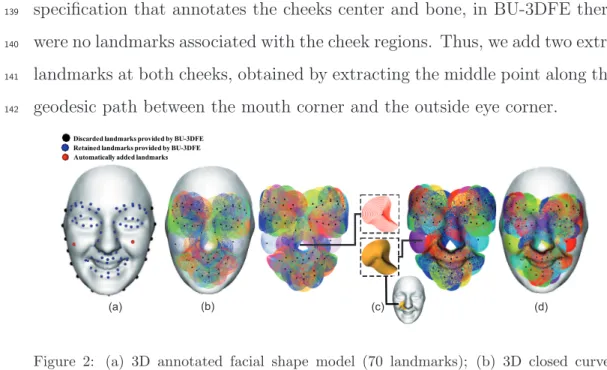
53
for 3D facial expression recognition, the first work related to this issue was
54
presented by Wang et al. [8]. They proposed a novel geometric feature based
55
facial expression descriptor, derived from an estimation of primitive surface
56
feature distribution. A labeling scheme was associated with their extracted
57
features, and they constructed samples that have been used to train and test
58
several classifiers. They reported that the highest average recognition rate
59
they obtained was 83%. They evaluated their approach not only on
frontal-60
view facial expressions of the BU-3DFE database, but they also tested its
61
robustness to non-frontal views. A second work was reported by Soyel and
62
Demirel [9] on the same database. They extracted six characteristic distances
63
between eleven facial landmarks, and using Neural Network architecture that
64
analysis the calculated distances, they classified the BU-3DFE facial scans
65
into 7 facial expressions including neutral expression. The average
recog-66
nition rate they achieved was 91.3%. Mpiperis et al. [10] proposed a joint
67
3D face and facial expression recognition using bilinear model. They fitted
68
both formulations, using symmetric and asymmetric bilinear models to
en-69
code both identity and expression. They reported an average recognition
70
rate of 90.5%. They also reported that the facial expressions of disgust and
71
surprise were well identified with an accuracy of 100%. Tang and Huang [11]
72
proposed an automatic feature selection computed from the normalized
Eu-73
clidean distances between two picked landmarks from 83 possible ones. Using
regularized multi-class AdaBoost classification algorithm, they reported an
75
average recognition rate of 95.1%, and they mentioned that the surprise
ex-76
pression was recognized with an accuracy of 99.2%.
77
In this paper, we further investigate the problem of 3D identity-independent
78
facial expression recognition. The main contributions of our approach are
79
the following: (1) We propose a new process for representing and extracting
80
patches on the facial surface scan that cover multiple regions of the face;
81
(2) We apply a framework to derive 3D shape analysis to quantify similarity
82
measure between corresponding patches on different 3D facial scans. Thus,
83
we combine a local geometric-based shape analysis approach of 3D faces and
84
several machine learning techniques to perform such classification.
85
3. Database Description
86
BU-3DFE is one of the very few publicly available databases of annotated
87
3D facial expressions, collected by Yin et al. [12] at Binghamton University.
88
It was designed for research on 3D human face and facial expression and to
89
develop a general understanding of the human behavior. Thus the BU-3DFE
90
database is beneficial for several fields and applications dealing with human
91
computer interaction, security, communication, psychology, etc. There are a
92
total of 100 subjects in the database, 56 females and 44 males. A neutral
93
scan was captured for each subject, then they were asked to perform six
94
expressions namely: Happiness (HA), Anger (AN), Fear (FE), Disgust (DI),
95
Sad (SA) and Surprise (SU). The expressions vary according to four levels
96
of intensity (low, middle, high and highest or 01-04). Thus, there are 25 3D
97
facial expression models per subject in the database. A set of 83 manually
annotated facial landmarks is associated to each model. These landmarks are
99
used to define the regions of the face that undergo to specific deformations
100
due to single muscles movements when conveying facial expression [7]. In
101
Fig. 1, we illustrate examples of the six universal facial expressions 3D models
102
including the highest intensity level.
Happy Angry Fear Disgust Sad Surprise
Figure 1: Examples of 3D facial expression models (first row 3D shape models, second row 3D textured models) of the BU-3DFE database.
103
4. 3D Facial Patches-based Representation
104
Most of the earlier work in 3D shape analysis use shape descriptors such as
105
curvature, crest lines, shape index (e.g., ridge, saddle, rut, dome, etc.). These
106
descriptors are defined based on the geometric and topological properties of
107
the 3D object, and are used as features to simplify the representation and
108
thus the comparison for 3D shape matching and recognition tasks. Despite
109
their rigorous definition, such features are computed based on numerical
110
approximation that involves second derivatives and can be sensitive to noisy
111
data. In case of 3D facial range models, the facial surface labeling is a
112
critical step to describe the facial behavior or expression, and a robust facial
surface representation is needed. In Samir et al. [13] the authors proposed
114
to represent facial surfaces by an indexed collections of 3D closed curves
115
on faces. These curves are level curves of a surface distance function (i.e.,
116
geodesic distance) defined to be the length of the shortest path between a
117
fixed reference point (taken to be the nose tip) and a point of the extracted
118
curve along the facial surface. This being motivated by the robustness of the
119
geodesic distance to facial expressions and rigid motions. Using this approach
120
they were able to compare 3D shapes by comparing facial curves rather than
121
comparing corresponding shape descriptors.
122
In our work we intend to further investigate on local shapes of the facial
123
surface. We are especially interested in capturing deformations of local facial
124
regions caused by facial expressions. Using a different solution, we compute
125
curves using the Euclidean distance which is sensitive to deformations and
126
thus can better capture differences related to variant expressions. To this
127
end, we choose to consider N reference points (landmarks) {rl}1≤l≤N (Fig.2
128
(a)) and associated sets of level curves {cl
λ}1≤λ≤λ0 (Fig.2 (b)). These curves
129
are extracted over the patches centered at these points. Here λ stands for the
130
value of the distance function between the reference point rl and the point
131
belonging to the curve cl
λ, and λ0 stands for the maximum value taken by
132
λ. Accompanying each facial model there are 83 manually picked landmarks,
133
these landmarks are practically similar to the MPEG-4 feature points and
134
are selected based on the facial anatomy structure. Given these points the
135
feature region on the face can be easily determined and extracted. We were
136
interested in a subset of 68 landmarks laying within the face area, discarding
137
those marked on the face border. Contrary to the MPEG-4 feature points
specification that annotates the cheeks center and bone, in BU-3DFE there
139
were no landmarks associated with the cheek regions. Thus, we add two extra
140
landmarks at both cheeks, obtained by extracting the middle point along the
141
geodesic path between the mouth corner and the outside eye corner.
142
Discarded landmarks provided by BU-3DFE Retained landmarks provided by BU-3DFE Automatically added landmarks
Figure 2: (a) 3D annotated facial shape model (70 landmarks); (b) 3D closed curves extracted around the landmarks; (c) 3D curve-based patches composed of 20 level curves with a size fixed by a radius λ0= 20mm; (d) Extracted patches on the face.
We propose to represent each facial scan by a number of patches centered
143
on the considered points. Let rl be the reference point and Pl a given patch
144
centered on this point and localized on the facial surface denoted by S. Each
145
patch will be represented by an indexed collection of level curves. To extract
146
these curves, we use the Euclidean distance function krl− pk to characterize
147
the length between rl and any point p on S. Indeed, unlike the geodesic
148
distance, the Euclidean distance is sensitive to deformations, and besides,
149
it permits to derive curve extraction in a fast and simple way. Using this
150
function we defined the curves as level sets of:
151
krl− .k : clλ = {p ∈ S | krl− pk = λ} ⊂ S, λ ∈ [0, λ0]. (1)
Each cl
λ is a closed curve, consisting of a collection of points situated at an
equal distance λ from rl. The Fig. 2 resumes the scheme of patches extraction.
153
5. Framework for 3D Shape Analysis
154
Once the patches are extracted, we aim at studying their shape and design
155
a similarity measure between corresponding ones on different scans under
156
different expressions. This is motivated by the common belief that people
157
smile, or convey any other expression, the same way, or more appropriately
158
certain regions taking part in a specific expression undergo practically the
159
same dynamical deformation process. We expect that certain corresponding
160
patches associated with the same given expression will be deformed in a
161
similar way, while those associated with two different expressions will deform
162
differently. The following sections describe the shape analysis of closed curves
163
in R3, initially introduced by Joshi et al. [3], and its extension to analyze
164
shape of local patches on facial surfaces.
165
5.1. 3D Curve Shape Analysis
166
We start by considering a closed curve β in R3. While there are several
167
ways to analyze shapes of closed curves, an elastic analysis of the parametrized
168
curves is particularly appropriate in 3D curves analysis. This is because (1)
169
such analysis uses a square-root velocity function representation which
al-170
lows us to compare local facial shapes in presence of elastic deformations,
171
(2) this method uses a square-root representation under which the elastic
172
metric reduces to the standard L2 metric and thus simplifies the analysis,
173
(3) under this metric the Riemannian distance between curves is invariant
174
to the re-parametrization. To analyze the shape of β, we shall represent it
175
mathematically using a square-root representation of β as follows ; for an
interval I = [0, 1], let β : I −→ R3 be a curve and define q : I −→ R3 to be
177
its square-root velocity function (SRVF), given by:
178
q(t) =. qβ(t)˙
k ˙β(t)k
. (2)
Here t is a parameter ∈ I and k.k is the Euclidean norm in R3. We
179
note that q(t) is a special function that captures the shape of β and is
par-180
ticularly convenient for shape analysis, as we describe next. The classical
181
elastic metric for comparing shapes of curves becomes the L2-metric under
182
the SRVF representation [14]. This point is very important as it
simpli-183
fies the calculus of elastic metric to the well-known calculus of functional
184
analysis under the L2-metric. Also, the squared L2-norm of q, given by:
185
kqk2 = R
S1 < q(t), q(t) > dt =
R
S1k ˙β(t)kdt , which is the length of β.
186
In order to restrict our shape analysis to closed curves, we define the set:
187
C = {q : S1 −→ R3|R
S1q(t)kq(t)kdt = 0} ⊂ L2(S1, R3). Notice that the
188
elements of C are allowed to have different lengths. Due to a non-linear
(clo-189
sure) constraint on its elements, C is a non-linear manifold. We can make it
190
a Riemannian manifold by using the metric: for any u, v ∈ Tq(C), we define:
191
hu, vi = Z
S1
hu(t), v(t)i dt . (3)
So far we have described a set of closed curves and have endowed it with a
192
Riemannian structure. Next we consider the issue of representing the shapes
193
of these curves. It is easy to see that several elements of C can represent
194
curves with the same shape. For example, if we rotate a curve in R3, we get a
195
different SRVF but its shape remains unchanged. Another similar situation
196
arises when a curve is re-parametrized; a re-parameterization changes the
SRVF of curve but not its shape. In order to handle this variability, we define
198
orbits of the rotation group SO(3) and the re-parameterization group Γ as
199
the equivalence classes in C. Here, Γ is the set of all orientation-preserving
200
diffeomorphisms of S1 (to itself) and the elements of Γ are viewed as
re-201
parameterization functions. For example, for a curve β : S1 → R3 and a
202
function γ : S1 → S1, γ ∈ Γ, the curve β ◦ γ is a re-parameterization of β.
203
The corresponding SRVF changes according to q(t) 7→p ˙γ(t)q(γ(t)). We set
204
the elements of the orbit:
205
[q] = {p ˙γ(t)Oq(γ(t))|O ∈ SO(3), γ ∈ Γ} , (4)
to be equivalent from the perspective of shape analysis. The set of such
206
equivalence classes, denoted by S = C/(SO(3) × Γ) is called the shape space.
207
of closed curves in R3. S inherits a Riemannian metric from the larger space
208
C due to the quotient structure.
209
The main ingredient in comparing and analysing shapes of curves is the
210
construction of a geodesic between any two elements of S, under the
Rieman-211
nian metric given in Eq.(3). Given any two curves β1 and β2, represented
212
by their SRVFs q1 and q2, we want to compute a geodesic path between the
213
orbits [q1] and [q2] in the shape space S. This task is accomplished using
214
a path-straightening approach which was introduced in [15]. The basic idea
215
here is to connect the two points [q1] and [q2] by an arbitrary initial path α
216
and to iteratively update this path using the negative gradient of an energy
217
function E[α] = 12R
sh ˙α(s), ˙α(s)i ds. The interesting part is that the gradient
218
of E has been derived analytically and can be used directly for updating α.
219
As shown in [15], the critical points of E are actually geodesic paths in S.
Thus, this gradient-based update leads to a critical point of E which, in turn,
221
is a geodesic path between the given points. In the remainder of the paper,
222
we will use the notation dS(β1, β2) to denote the length of the geodesic in the
223
shape space S between the orbits q1 and q2, to reduce the notation.
224
5.2. 3D Patches Shape Analysis
225
Now, we extend ideas developed in the previous section from analyzing
226
shapes of curves to the shapes of patches. As mentioned earlier, we are going
227
to represent a number of l patches of a facial surface S with an indexed
228
collection of the level curves of the krl− .k function (Euclidean distance from
229
the reference point rl). That is, Pl ↔ {clλ, λ ∈ [0, λ0]} , where c
l
λ is the level
230
set associated with krl− .k = λ. Through this relation, each patch has been
231
represented as an element of the set S[0,λ0]. In our framework, the shapes of
232
any two patches are compared by comparing their corresponding level curves.
233
Given any two patches P1 and P2, and their level curves {c1λ, λ ∈ [0, λ0]} and
234
{c2
λ, λ ∈ [0, λ0]}, respectively, our idea is to compare the patches curves c1λ
235
and c2
λ, and to accumulate these differences over all λ. More formally, we
236
define a distance dS[0,λ0] given by:
237
dS[0,λ0](P1, P2) =
Z L
0
dS(c1λ, c2λ)dλ . (5)
In addition to the distance dS[0,λ0](P1, P2), which is useful in biometry
238
and other classification experiments, we also have a geodesic path in S[0,λ0]
239
between the two points represented by P1 and P2. This geodesic corresponds
240
to the optimal elastic deformations of facial curves and, thus, facial surfaces
241
from one to another. Fig. 3 shows some examples of geodesic paths that
242
are computed between corresponding patches associated with shape models
convex concave
Target
Reference Query
Source
Figure 3: Examples of intra-class (same expression) geodesic paths with shape and mean curvature mapping between corresponding patches.
sharing the same expression, and termed intra-class geodesics. In the first
244
column we illustrate the source, which represents scan models of the same
245
subject, but under different expressions. The third column represents the
246
targets as scan models of different subjects. As for the middle column, it
247
shows the geodesic paths. In each row we have both the shape and the
248
mean curvature mapping representations of the patches along the geodesic
249
path from the source to the target. The mean curvature representation is
250
added to identify concave/convex areas on the source and target patches and
equally-spaced steps of geodesics. This figure shows that certain patches,
252
belonging to the same class of expression, are deformed in a similar way.
253
In contrast, Fig. 4 shows geodesic paths between patches of different facial
254
expressions. These geodesics are termed inter-class geodesics. Unlike the
255
intra-class geodesics shown in Fig. 3, these patches deform in a different way.
256 convex concave Target Reference Query Source
Figure 4: Examples of inter-class (different expressions) geodesic paths between source and target patches.
6. Feature Vector Generation for Classification
257
In order to classify expressions, we build a feature vector for each facial
258
scan. Given a candidate facial scan of a person j, facial patches are extracted
259
around facial landmarks. For a facial patch Pi
j, a set of level curves {cλ}ij are
260
extracted centered on the ith landmark. Similarly, a patch Pi
ref is extracted
261
in correspondence to landmarks of a reference scans ref. The length of the
262
geodesic path between each level curve and its corresponding curve on the
reference scan are computed using a Riemannian framework for shape
anal-264
ysis of 3D curves (see Sections 5.1 and 5.2). The shortest path between two
265
patches at landmark i, one in a candidate scan and the other in the reference
266
scan, is defined as the sum of the distances between all pairs of corresponding
267
curves in the two patches as indicated in Eq. (5). The feature vector is then
268
formed by the distances computed on all the patches and its dimension is
269
equal to the number of used landmarks N = 70 (i.e., 68 landmarks are used
270
out of the 83 provided by BU-3DFED and the two additional cheek points).
271
The ith element of this vector represents the length of the geodesic path that
272
separates the relative patch to the corresponding one on the reference face
273
scan. All feature vectors computed on the overall dataset will be labeled and
274
used as input data to machine learning algorithms such as Multi-boosting
275
and SVM, where Multi-boosting is an extension of the successful Adadoost
276
technique for forming decision committees.
277
7. Recognition Experiments
278
To investigate facial expression recognition, we have applied our proposed
279
approach on a dataset that is appropriate for this task. In this Section,
280
we describe the experiments, obtained results and comparisons with related
281
work.
282
7.1. Experimental Setting
283
For the goal of performing identity-independent facial expression
recog-284
nition, the experiments were conducted on the BU-3DFE static database. A
285
dataset captured from 60 subjects were used, half (30) of them were female
286
and the other half (30) were male, corresponding to the high and highest
intensity levels 3D expressive models (03-04). These data are assumed to be
288
scaled to the true physical dimensions of the captured human faces.
Follow-289
ing a similar setup as in [16], we randomly divided the 60 subjects into two
290
sets, the training set containing 54 subjects (648 samples), and the test set
291
containing 6 subjects (72 samples).
292
To drive the classification experiments, we arbitrarily choose a set of six
293
reference subjects with its six basic facial expressions. We point out that
294
the selected reference scans do not appear neither in the training nor in the
295
testing set. These references, shown in Fig. 5, with their relative expressive
296
scans corresponding to the highest intensity level, are taken to play the role
297
of representative models for each of the six classes of expressions. For each
298
reference subject, we derive a facial expression recognition experience.
299
7.2. Discussion of the Results
300
Several facial expression recognition experiments were conducted with
301
changing at each time the reference. Fig. 5 illustrates the selected references
302
(neutral scan). Using the Waikato Environment for Knowledge Analysis
303
(Weka) [17], we applied the Multiboost algorithm with three weak
classi-304
fiers, namely, Linear Discriminant Analysis (LDA), Naive Bayes (NB), and
305
Nearest Neighbor (NN), to the extracted features, and we achieved average
306
recognition rates of 98.81%, 98.76% and 98.07%, respectively. We applied
307
the SVM linear classifier as well, and we achieved an average recognition rate
308
of 97.75%. We summarize the resulting recognition rates in Table 1.
309
We note that these rates are obtained by averaging the results of the
310
10 independent and arbitrarily run experiments (10-fold cross validation)
311
and their respective recognition rate obtained using the Multiboost-LDA
Table 1: Classification results using local shape analysis and several classifiers.
Classifier Multiboost-LDA Multiboost-NB Multiboost-NN SVM-Linear
Recognition rate 98.81% 98.76% 98.07% 97.75%
classifier. We note that different selections of the reference scans do not
313
affect significantly the recognition results and there is no large variations in
314
recognition rates values. The reported results represent the average over the
315
six runned experiments. The Multiboost-LDA classifier achieves the highest
316
recognition rate and shows a better performance in terms of accuracy than
317
the other classifiers. This is mainly due to the capability of the LDA-based
318
classifier to transform the features into a more discriminative space and,
319
consequently, result in a better linear separation between facial expression
320 classes. 321 99.86% 99.86% 1 2 3 4 5 6 50 60 70 80 90 100 110 120 References
Average Recognition Rate (%)
99.86 99.58 98.88 98.61 98.05 97.91
Figure 5: Different facial expression average recognition rates obtained using different reference subjects (using Multiboost-LDA).
The average confusion matrix relative to the the best performing
fication using Multiboost-LDA is given in Table 2.
Table 2: Average confusion matrix given by Multiboost-LDA classifier.
% AN DI FE HA SA SU AN 97.92 1.11 0.14 0.14 0.69 0.0 DI 0.56 99.16 0.14 0.0 0.14 0.0 FE 0.14 0.14 99.72 0.0 0.0 0.0 HA 0.56 0.14 0.0 98.60 0.56 0.14 SA 0.28 0.14 0.0 0.0 99.30 0.28 SU 0.14 0.56 0.0 0.0 1.11 98.19 323
In order to better understand and explain the results mentioned above,
324
we apply the Multiboost algorithm on feature vectors built from distances
325
between patches for each class of expression. In this case, we consider these
326
features as weak classifiers. Then, we look at the early iterations of the
327
Multiboost algorithm and the selected patches in each iteration.
328
Happy Angry Fear Disgust Sad Surprise
0.0207 0.0149 0.0143 0.0139 0.0123 0.0117 0.0214 0.0161 0.0146 0.0137 0.0123 0.0118 0.0189 0.0187 0.0175 0.0170 0.0137 0.0128 0.0290 0.0142 0.0141 0.0123 0.0120 0.0118 0.0176 0.0164 0.0157 0.0151 0.0148 0.0142 0.0187 0.0165 0.0163 0.0138 0.0134 0.0127
Figure 6: Selected patches at the early few iterations of Multiboost classifier for the six facial expressions (Angry, Disgust, Fear, Happy, Sadness, Surprise) with their associated weights.
Fig. 6 illustrates for each class of expression the most relevant patches.
329
Notice that, for example, for the Happy expression the selected patches are
330
localized in the lower part of the face, around the mouth and the chin. As
for the Surprise expression, we can see that most relevant patches are
lo-332
calized around the eyebrows and the mouth region. It can be seen that
333
patches selected for each expression lie on facial muscles that contribute to
334
this expression.
335
7.3. Comparison with Related Work
336
In Table 3 results of our approach are compared against those reported
337
in [11], [9], and [8], on the same experimental setting (54-versus-6-subject
338
partitions) of the BU-3DFE database. The differences between approaches
339
should be noted: Tang et al. [11] performed automatic feature selection
us-340
ing normalized Euclidean distances between 83 landmarks, Soyel et al. [9]
341
calculated six distances using a distribution of 11 landmarks, while Wang et
342
al. [8] derived curvature estimation by locally approximating the 3D surface
343
with a smooth polynomial function. In comparison, our approach capture
344
the 3D shape information of local facial patches to derive shape analysis.
345
For assessing how the results of their statistical analysis will generalize to
346
an independent dataset, in [8] a 20-fold cross-validation technique was used,
347
while in [11] and [9] the authors used 10-fold cross-validation to validate their
348
approach.
349
Table 3: Comparison of this work with respect to previous work [11], [9] and [8].
Cross-validation This work Tang et al. [11] Soyel et al. [9] Wang et al. [8]
10-fold 98.81% 95.1% 91.3%
7.4. Non-frontal View Facial Expression Recognition
350
In real world situations, frontal view facial scans may not be always
avail-351
able. Thus, non-frontal view facial expression recognition is a challenging
is-352
sue that needs to be treated. We were interested in evaluating our approach
353
on facial scan under large pose variations. By rotating the 3D shape
mod-354
els in the y-direction, we generate facial scans under six different non-frontal
355 views corresponding to 15◦ , 30◦ , 45◦ , 60◦ , 75◦ and 90◦ rotation. We assume 356
that shape information is unavailable for the occluded facial regions due to
357
the face pose. For each view, we perform facial patches extraction around the
358
visible landmarks in the given scan. In cases where a landmark is occluded,
359
or where the landmark is visible, but the region nearby is partially occluded,
360
we treat it as a missing data problem for all faces sharing this view. In these
361
cases, we are not able to compute the geodesic path between corresponding
362
patches. The corresponding entries in the distance matrix are blank and we
363
fill them using an imputation technique [18]. In our experiments we employed
364
the mean imputation method, which consists of replacing the missing values
365
by the means of values already calculated in frontal-view scenario obtained
366
from the training set. Let dijk = dS[0,λ0](Pik, Pjk) be the geodesic distance
be-367
tween the kth patch belonging to subjects i and j (i 6= j). In case of frontal
368
view (f v), the set of instances Xif v relative to the subject i need to be labeled
and is given by: 370 Xfvi =
di11 . . . di1k . . . di1N
... ... ... ... ...
dij1 . . . dijk ... dijN
... ... ... ... ... diJ1 . . . diJ k . . . diJ N
where N is the number of attributes. In case of non-frontal view (nf v), if
371
an attribute k is missing, we replace the kth column vector in the distance
372
matrix Xinf v by the mean of geodesic distances computed in the frontal-view
373
case, with respect to the kth attribute and given by: mf v
k =
PJ
j=1dijk
J , where
374
J is the total number of instances.
375 Xnfvi = di11 . . . mf vk . . . di1N ... ... ... ... ... dij1 . . . mf vk ... dijN ... ... ... ... ... diJ1 . . . mf vk . . . diJ N
To evaluate the robustness of our approach in a context of non-frontal views,
376
we derive a view-independent facial expression recognition. Error recognition
377
rates are evaluated throughout different testing facial views using the four
378
classifiers trained only on frontal-view facial scans. The Fig. 7 shows the
379
average error rates of the four classification methods. The Multiboost-LDA
380
shows the best performance for facial expression classification on the chosen
381
database. From the figure, it can be observed that the average error rates
382
increase with the rotation angle (values from 0 to 90 degrees of rotation are
383
considered), and the Multiboost-LDA is the best performing methods also
in the case of pose variations. As shown in this figure, recognition accuracy
385
remains acceptable, even only 50% of data (half face) are available when we
386
rotate the 3D face by 45 degree in y-direction.
387 0 15 30 45 60 75 90 10 20 30 40 50 60 70 80 90 100 110 View (°)
Average Error Rate (%)
Available data Multiboost−LDA Multiboost−NB Multiboost−NN SVM−Linear 42% 32% 14% 67% 80% 100% 50%
Figure 7: The average error rates of six expressions with different choice of views corre-sponding to the best reference and using different classifiers.
7.5. Sensitivity to Landmarks Mis-localization
388
It is known that the automatic 3D facial feature points detection is a
chal-389
lenging problem. The most difficult task remains the localization of points
390
around the eyebrow regions, which appear to play an important role in the
391
expression of emotions. The effect of the mis-localization of the landmarks
392
has been addressed in a specific experiment. We considered the eyebrow
re-393
gions in that the points in these regions are expected to be the most difficult
to detect automatically. In these regions, we added noise to the landmarks
395
provided with the BU-3DFED. In particular, we added noise to the position
396
of the landmarks by moving them randomly in a region with a radius of
397
10mm, as illustrated Fig. 8 by blue circles. Then we performed expression
398
recognition experiments with such noisy landmarks. The results are reported
399
in Fig. 8. It can be noted that with the Multiboost-LDA algorithm the lower
400
decrease in the recognition rate is observed, and even with a recognition rate
401
equal to 85.64% the result still outperforms the one reported in Wang et al
402 [8]. 79.22 80.74 82.52 98.81 98.76 98.07 97.75 85.64
Figure 8: Recognition experiment performed adding noise to the eyebrow landmarks (ran-dom displacement).
403
8. Conclusions
404
In this paper we presented a novel approach for identity-independent
fa-405
cial expression recognition from 3D facial shapes. Our idea was to describe
406
the change in facial expression as a deformation in the vicinity of facial
407
patches in 3D shape scan. An automatic extraction of local curve based
patches within the 3D facial surfaces was proposed. These patches were used
409
as local shape descriptors for facial expression representation. A Riemannian
410
framework was applied to compute the geodesic path between
correspond-411
ing patches. Qualitative (inter and intra-geodesic paths) and quantitative
412
(geodesic distances) measures of the geodesic path were explored to derive
413
shape analysis. The geodesic distances between patches were labeled with
414
respect to the six prototypical expressions and used as samples to train and
415
test machine learning algorithms. Using Multiboost algorithm for multi-class
416
classification, we achieved a 98.81% average recognition rate for six
proto-417
typical facial expressions on the BU-3DFE database. We demonstrated the
418
robustness of the proposed method to pose variations. In fact, the obtained
419
recognition rate remain acceptable (over 93%) even half of the facial scan is
420
missed.
421
The major limitation of our approach is that the 68 landmarks we used to
422
define the facial patches were manually labeled. For our future work we
423
are interested in detecting and tracking facial feature points, as proposed
424
in [19], [20], for automatic 3D facial expression recognition.
425
References
426
[1] P. Ekman, T. S. Huang, T. J. Sejnowski, J. C. Hager, Final report to
427
nsf of the planning workshop on facial expression understanding, Tech.
428
rep., available from Human Interaction Lab, LPPI Box 0984, University
429
of California, San Francisco, CA 94143 (1992).
430
[2] P. Ekman, W. V. Friesen, Constants Across Cultures in the Face and
431
Emotion (1971).
[3] S. Joshi, E. Klassen, A. Srivastava, I. H. Jermyn, A novel representation
433
for riemannian analysis of elastic curves in Rn, in: Proc. IEEE Computer
434
Vision and Pattern Recognition (CVPR), 2007.
435
[4] M. Pantic, L. Rothkrantz, Automatic analysis of facial expressions: The
436
state of the art, IEEE Transactions on Pattern Analysis and Machine
437
Intelligence 22 (12) (2000) 1424–1445.
438
[5] A. Samal, P. A. Iyengar, Automatic recognition and analysis of human
439
faces and facial expressions: a survey, Pattern Recognition 25 (1) (1992)
440
65–77.
441
[6] J. Whitehill, C. W. Omlin, Local versus global segmentation for facial
442
expression recognition, in: FGR ’06: Proceedings of the 7th
Interna-443
tional Conference on Automatic Face and Gesture Recognition, 2006,
444
pp. 357–362.
445
[7] P. Ekman, W. Friesen, Facial Action Coding System: A Technique for
446
the Measurement of Facial Movement, consulting Psychologists Press
447
(1978).
448
[8] J. Wang, L. Yin, X. Wei, Y. Sun, 3d facial expression recognition based
449
on primitive surface feature distribution, IEEE Conference on Computer
450
Vision and Pattern Recognition (CVPR) (2006) 1399–1406.
451
[9] H. Soyel, H. Demirel, Facial expression recognition using 3d facial feature
452
distances, International Conference on Image Analysis and Recognition
453
(ICIAR) (2007) 831–838.
[10] I. Mpiperis, S. Malassiotis, M. G. Strintzis, Bilinear models for 3d face
455
and facial expression recognition, IEEE Transactions on Information
456
Forensics and Security 3 (3) (2008) 498–511.
457
[11] H. Tang, T. Huang, 3d facial expression recognition based on
automat-458
ically selected features, In First IEEE Workshop on CVPR for Human
459
Communicative Behavior Analysis (CVPR4HB) (2008) 1–8.
460
[12] L. Yin, X. Wei, Y. Sun, J. Wang, M. J. Rosato, A 3d facial expression
461
database for facial behavior research, in: FGR ’06: Proceedings of the
462
7th International Conference on Automatic Face and Gesture
Recogni-463
tion, 2006, pp. 211–216.
464
[13] C. Samir, A. Srivastava, M. Daoudi, E. Klassen, An intrinsic framework
465
for analysis of facial surfaces, International Journal of Computer Vision
466
82 (1) (2009) 80–95.
467
[14] A. Srivastava, E. Klassen, S. H. Joshi, I. H. Jermyn, Shape analysis of
468
elastic curves in euclidean spaces, IEEE Transactions on Pattern
Anal-469
ysis and Machine Intelligence accepted for publication.
470
[15] E. Klassen, A. Srivastava, Geodesics between 3d closed curves using
471
path-straightening, in: ECCV (1), 2006, pp. 95–106.
472
[16] B. Gong, Y. Wang, J. Liu, X. Tang, Automatic facial expression
recogni-473
tion on a single 3D face by exploring shape deformation, in: Proceedings
474
of the ACM International Conference on Multimedia, Beijing, China,
475
2009, pp. 569–572.
[17] M. Hall, E. Frank, G. Holmes, B. Pfahringer, P. Reutemann, I. H.
477
Witten, The weka data mining software: An update, SIGKDD Explor.
478
Newsl 11 (2009) 10–18.
479
[18] G. Batista, M. C. Monard, An analysis of four missing data treatment
480
methods for supervised learning, Applied Artificial Intelligence 17 (2003)
481
519–533.
482
[19] S. Gupta, M. K. Markey, A. C. Bovik, Anthropometric 3d face
recogni-483
tion, International Journal of Computer Vision.
484
[20] Y. Sun, X. Chen, M. Rosato, L. Yin, Tracking vertex flow and model
485
adaptation for three-dimensional spatiotemporal face analysis, IEEE
486
Transactions on Systems, Man, and Cybernetics–Part A 40 (3) (2010)
487
461–474.