HAL Id: hal-00838969
https://hal.inria.fr/hal-00838969
Submitted on 26 Jun 2013
HAL is a multi-disciplinary open access
archive for the deposit and dissemination of
sci-entific research documents, whether they are
pub-lished or not. The documents may come from
teaching and research institutions in France or
abroad, or from public or private research centers.
L’archive ouverte pluridisciplinaire HAL, est
destinée au dépôt et à la diffusion de documents
scientifiques de niveau recherche, publiés ou non,
émanant des établissements d’enseignement et de
recherche français ou étrangers, des laboratoires
publics ou privés.
Alarms correlation in telecommunication networks
Anne Bouillard, Aurore Junier, Benoit Ronot
To cite this version:
Anne Bouillard, Aurore Junier, Benoit Ronot. Alarms correlation in telecommunication networks.
[Research Report] RR-8321, INRIA. 2013, pp.17. �hal-00838969�
0249-6399 ISRN INRIA/RR--8321--FR+ENG
RESEARCH
REPORT
N° 8321
June 2013Alarms correlation in
telecommunication
networks
RESEARCH CENTRE
RENNES – BRETAGNE ATLANTIQUE
networks
Anne Bouillard
∗, Aurore Junier
†, Benoit Ronot
‡Project-Teams SUMO and TREC
Research Report n° 8321 — June 2013 — 17 pages
Abstract: Nowadays telecommunication systems are growing more and more complex, gen-erating huge amount of alarms that cannot be effectively managed by human operators. The problematic is to detect in real-time significant combinations of alarms that describe an issue. In this article, we present a powerful heuristic algorithm that constructs alarm patterns dependency graphs. More precisely, it is able to highlight patterns extracted from an alarm flow learning process with a small footprint on network management system performance. This algorithm is first relevant to real-time issues detection by effectively delivering their concise alarm patterns. And secondly it allows the proactive analysis of network health by retrieving the general trends of a network. We challenge our algorithm to an optical network alarms data set of an existing operator. We find immediately similar results to the experts analysis performed for this operator by Alcatel-Lucent Customer Services.
Key-words: management methods, proactive systems, alarms correlation
∗ENS / INRIA, TREC, [email protected] †INRIA / IRISA, SUMO, [email protected]
Corr´
elation des alarmes dans les r´
eseaux de
t´
el´
ecommunication
R´esum´e : De nos jours, les syst`emes de t´el´ecommunication deviennent de plus en plus complexes, g´en´erant une quantit´e d’alarmes ´enorme qui ne peut ˆetre efficacement g´er´ee par un humain. Le probl`eme est de d´etecter en temps-r´eel des combinaisons d’alarmes d´ecrivant un probl`eme. Dans cet article, nous pr´esentons un puissant algorithme heuristique construisant un graphe de d´ependances contenant des motifs d’alarmes. Plus pr´ecis´ement, cet algorithme est capable d’extraire des motifs `a partir d’un flot d’alarmes observ´ees en ayant un faible impact sur les performances des syst`emes de management. Tout d’abord, cet algorithme est tr`es pertinent pour d´etecter des probl`emes temps-r´eel car il d´elivre des motifs d’alarmes concis. Deuxi`emement, il permet une analyse proactive de la sant´e du r´eseau par l’extraction de la tendance g´en´erale d’un r´eseau. Nous testons notre algorithme sur un ensemble d’alarmes g´en´er´e par un r´eseau optique d’un op´erateur existant. Nous avons imm´ediatement trouv´e des r´esultats similaires `a ceux obtenus, pour cet op´erateur, par les experts du service client d’Alcatel-Lucent.
1
Introduction
Network management, especially for issue resolution has become in the last decade a very complex task, requiring high human expertise and complex tools for network context analysis. To face the increasing networks complexity, alarm varieties have been expended, most of them referring no longer to any critical problem ([12]). Networks are producing thousands of alarms a day which can no longer be effectively managed by human operators. Furthermore, it has been presented ([13]) that this huge quantity is highly redundant: a single fault can have several symptoms, can be propagated, or can have a long duration, which generates several alarms. Moreover the introduction of new technologies such as Autonomic Network processes and Software Defined Networks will not alleviate tomorrow’s network management problems.
The principle of alarm correlation is to group alarms referring to the same problem (to reduce redundancy) and to highlight those referring to probable faults that might drive the network into a dangerous state. There are many studies in the recent years (see section 2) that respond to these challenges, some based on alarm correlation ([8]) or on alarm pattern retrieval algorithm ([7]). But both approaches have their limits. The first type implies too complexity to adapt to any network context. Also, the fact that temporal patterns can be doomed to failure by the inversion of alarms due to the network management system (NMS) logging process or a different equipment configuration is a limit to apply the second type of method. Therefore, automatic techniques that process the huge quantity of alarms are now compulsory to build reliable networks.
In this paper, we present a new heuristic algorithm that constructs alarm patterns dependency graphs. Our aim is to develop an efficient method that can be applied to all kind of networks without making assumptions about the characteristics of the network. Our research is based on the assumption that the alarms that mostly occur in the network are those referring to general information about the network. As a consequence, we focus our study on the observation of non-frequent alarms.
The paper is organized as follows. In Section 2, we discuss related work. Section 3 introduces the method that defines patterns of non-frequent alarms. Based on these patterns, dependency graphs are constructed to identify alarms that might lead to a major faulty behavior. These graphs also highlight if a solution has been provided (Section 4). In section 5, we introduce an earlier work. We show that applying this method helps by giving an overall knowledge of the network behavior. Finally, we show the evaluation and the results of the proposed method in Section 6.
2
State of the art
Many approaches have been proposed to address the problem of alarm correlation in networks over the last three decades. Here, we present an overview of some existing correlation techniques. Method based on graph dependency: The heuristic algorithm proposed in [15] was a pioneer in alarm correlation to find the root cause of anomalies. It constructs a statistical dependency graph of the network elements (nodes, links). Based on this graph, it builds for each alarm that appears in the system the domain of the alarm (set of objects that might have caused the alarm) which is a variation of the single source problem. Finally, it presents and compares a set of localization algorithms based on this graph.
Methods based on specific architecture: Several articles design a correlation engine directly in the NMS. The idea is to improve some aspects of the NMS to reduce the raw flow of alarms observed by only sending the most pertinent information. Some methods ([19], [14]) define an alarm architecture using the principle of Model-Based Reasoning [6]. These methods introduce rule-based approaches to group alarms that refer to the same problem. IMPACT ([14])
4 Bouillard & Junier & Ronot
uses the ARTIM forward-rule-chaining algorithm to perform the alarm correlation from events occurring in the network. The Alarm Correlation Engine of Northern Telecom ([19]) has been implemented in Smalltalk and contains rule writers to maintain the knowledge of the network (i.e. the set of rules that defines a specific problem). The method introduced in [5] focuses on intelligent agents and inserts a correlation agent, based on the INFOSEC system architecture. The correlation agent generates an alarm if the weighted sum of the occurred alarms depending on their severity is up to a threshold. Another example is [1], where the authors provide a correlation system divided in three layers. Here, the traffic is characterized by using the Baseline for Automatic Backbone Management (BLGBA) model [21] that generates a normal behavior profile (DSNS: Digital Signature of Network Segment [16]). In a first time, the preprocessing layer builds a compact set of new alarms, called Device Level Alarms (DLA), by taking into account spatial and temporal information. Then, the correlation layer constructs a network dependency graph to represent dependencies between devices and identifies (by a heuristic algorithm) the source and the destination of anomalies. Finally, a presentation layer provides a visualization of paths in the graph affected by anomalies.
Method based on linear algebra: The technique proposed in [13] mathematically evalu-ates the redundancy of alarms. An alarm is defined as redundant to another one if it happens close in time to the other for most of the occurrences. The occurrence of an alarm is represented by a Gaussian centered on the actual occurrence time. A linear computation is performed to detect redundancies. However, this approach doesn’t take into account the alarms occurring between alarms designated as redundant, which gives additional important information.
Method based on pattern definition: Another way to correlate alarms is to create patterns of frequent alarms. This is the aim of studies [7], [10] and [11]. The principle is to perform data mining on the flow of alarms to define sequences that are temporally correlated. However the search of temporal patterns can be expensive in computation time. For example, in [7], the authors present an example that takes 2 mn to analyze a file of 2900 alarms of 36 different types.
Method based on probabilistic finite state machine: The method described in [17] correlates the alarms using probabilistic finite state machines (PFSM) describing faults. A PFSM represents the succession of alarms that imply a particular problem. The weakness in this approach is that the set of faults occurring in the network must be known in advance, as a PFSM is constructed for each fault at the beginning of the process. This is a problem as, since faults can come from anywhere, the set of faults can potentially be large.
Method based on correlation coefficient: The authors of article [9] present an off-line method based on statistics. The alarms are represented by Gaussian functions and the Pearson coefficient [20] is used to correlate them. Then, the links between alarms are represented on a colored map [18].
Until now, many methods have been suggested to correlate alarms in networks. The main difficulty resides in the ability to deal with a huge quantity of data to detect dangerous network behavior. Some methods use powerful mathematics tools that actually remain too complex. Other methods suggest new management tools based on a specific topology or assume some network characteristics. Here we introduce a generic method that efficiently creates several dependency graphs of alarms, based on the sequence of alarm names, that permits a quick study of the alarm correlation problem.
3
Construction of relevant patterns
Let us study a flow of alarms. We denote by A the set of alarms and a flow f is a finite sequence of alarms, f ∈ A∗. In the study the size of A is approximately 20, and |f |, the length of f , approximately 105
. Therefore, some alarms will appear very frequently, but some others will only appear a few times. Let us first focus on the latter ones.
We use the notations from the languages theory: if A is a finite set, we denote by A∗ the set of finite sequences with elements in A and by A+
the set of non-empty finite sequences with elements in A. If f ∈ A, then |f | is the length of f for a ∈ A,|f |a, is the number of occurrences of a in f . The symbol ’·’ stands for the concatenation: if f1 = a1· · · ai and f2 = b1· · · bj, then f1· f2= a1· · · aib1· · · bj. For f ∈ A∗, f is the support of f : f = {a ∈ A | |f |a ≥ 1}.
Our goal is to exhibit a group of non-frequent alarms that are correlated. In this aim, we perform the following transformations on the flow.
a) Identify the most frequent alarms M .
b) Cut f in a sequence of small set-patterns, sp(f ) using alarms in M as separators. c) Study the correlation between those set-patterns and reduce sp(f ).
Identification of the most frequent alarms This is simply done by counting the number of occurrences of each alarm a ∈ A that appears in f , |f |a, and using a fix threshold α. Then the set of frequent alarms is defined by
M = {a ∈ A | |f |a/|f | ≥ α}.
Construction of set-patterns In the sequence of alarms we study, some alarms are sent several times. So if an alarm a arrives before an alarm b, this does not always mean that a is the cause of b or that a has been generated before b. Moreover, we may often find patterns ababa... in the log-file. Also, the alarms are temporarily buffered by the system before being monitored. Consequently, the exact order between the alarms has a weaker impact than for a real-time monitoring, that is rare and expensive in infrastructure costs. As a consequence, for alarms that are consecutive or almost consecutive, we may not have to keep them ordered and short patterns (factors) of f can be considered as set of alarms instead of sequences.
Set R = A/M the set of alarms we focus on. Then f can be written as f = m0· r1· m1· r2· · · rℓ· mℓ,
where m0, mℓ ∈ M∗, m1, . . . , mℓ−1 ∈ M+, and r1, . . . , rℓ ∈ R+. Note that the mi and rj and uniquely defined.
We then obtain our set of set-patterns as
sp(f ) = r1· r2· · · rℓ∈ P(R)∗.
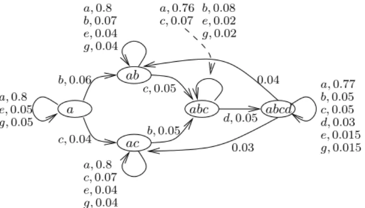
Example 1 Let’s consider an example with 6 alarms, A = {a, b, c, d, e, g}. Assume that alarm a is frequent, and that the occurrence of alarms b and c finally lead to the occurrence of alarm d. When d occurs, the fault associated to it is repaired, implying the stopping of alarms b and d, but not a and c. Alarms e and g are not related to fault resulting in alarm d and appear constantly at a small rate.
In order to generate an alarm log-file corresponding to this phenomenon, we use the Markov generator of Figure 1. The arcs are labeled by probabilities and the alarm that is generated. Let’s
6 Bouillard & Junier & Ronot a ab ac abc abcd b,0.06 c,0.04 c,0.05 c,0.07 e,0.04 g,0.04 g,0.04 e,0.04 b,0.07 a,0.8 d,0.05 b,0.05 a,0.8 a,0.77 b,0.05 c,0.05 d,0.03 e,0.015 g,0.015 0.03 0.04 a,0.8 e,0.05 g,0.05 a,0.76 b, 0.08 c,0.07 e, 0.02 g,0.02
Figure 1: Markov generator fr Example 1.
note that the probability of generating e or g decreases to model that the frequency of b and c increases after their first generations.
If the threshold α used to separate A into M and R is set to 0.5, then M = {a} and R = {b, c, d, e, g}.
We generate f of length 1000 using this generator, and observe that alarm d appears mostly as a singleton, but also in sets {b, d} and {c, d} quite frequently. It also appears in sets {e, d} or {g, d} or in larger sets, but much less frequently, as our model suggests it.
In our experiment, we get |sp(f )| = 180, which is still too large for a quick analysis.
We can also observe that many alarms are repeated, and the rarest alarm d appears in only 23 set-patterns. We need to have a much more schematic view of the dependency graph. Reducing the set-patterns The third step consists in reducing the length of |sp(f )|. This can be done by setting transformation rules. For u, v ∈ P(A),
(R1) uvu → u ∪ v (R2) uv → u if v ⊆ u.
In other words, if sp(f ) can be written as z1·uvu·z2, then we can transform it into z1·(u∪v)·z2 (rule (R1)), and if v ⊆ u and sp(f ) = z1· uv · z2, then we can transform it into z1· u · z2 (rule (R2)).
We can recursively apply those rules until no rule can be applied. Note that the application of those rules is not commutative, specially concerning (R1). For example, if we consider the sequence of set-pattern {b, d}{b}{c}{b}, rules (R1) and (R2) can apply, but using (R1) leads to {b, d}{b, c} and (R2) cannot be applied any more; using (R2) leads to {b, d}, {c}{b} and (R1) cannot be applied any more;
We arbitrary chose repeatedly to apply first rule (R1) from left to right and then (R2) until no rule can be used. We denote by rsp(f ) the reduced set-pattern obtained after applying rules (R1) and (R2).
Example 2 After the application of those rules to sp(f ) of Example 1, its length is reduced to 93. The reduction is not drastic because the number of alarms is too small. In Section 6, the reduction of the length will be more spectacular.
4
Relevant patterns detection
In this section, we use the heuristic of the previous section in order to find patterns leading to rare alarms. Rare alarms only appear a few times in the log-file: this corresponds to alarms that led to a major faulty behavior of the system and are often repaired very soon after the occurrence of the alarm. Identifying patterns leading to that fault may then allow a proactive management by detecting the root cause of a problem before it implies a failure.
In order to handle this, we construct the dependency graph G = (V, E, w) of the set-patterns found with our heuristic: G is a weighted directed graph with set of vertexes V , set of edges E and weight w : E → N, where
V = rsp(f), the set-patterns that appear in rsp(f); E = {(u, v) | ∃z1, z2 such that sp(f ) = z1· uv · z2;
w(u, v) = |{(z1, z2) | sp(f ) = z1· uv · z2}|, the number of occurrences of uv in rsp(f ). Now, we want to identify the alarms that (probably) led to a given alarm.
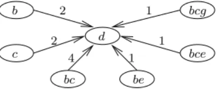
Example 3 The graph obtained in our example is too large to be represented. However, we can1 focus, for example on the rare alarm {d} and its predecessors. This is represented on Figure 2. We observe that all of the preceding contain b or c, and only a few contain e or g. This is in accordance with our generator that mostly generates b or c before the occurrence of an alarm d.
b c bc be bce 2 2 4 1 1 1 d bcg
Figure 2: Vertex {d} and its predecessors.
A difficulty in analyzing the flow of alarms resides in the fact that the alarms are registered on long periods of time (e.g. a year). Obviously, during a year, many events occur in a network and we focus on very few rare alarms, that occur at several times during this year. The immediate study of the dependency graph might be tough, as the time dependency between the alarms might be lost and also because the occurrence of those few rare alarms might correspond to different pathologies.
To address this problem the dependency graph is divided in sub-graphs, each focusing on the study of a rare alarm, or a set of rare alarms if they are strongly correlated. Each sub-graph represents a short successions of set-patterns occurred before and after the rare alarms considered. Observing this graph gives a refined analysis of the rare alarms. This provides hypotheses about the root cause that generated the alarms. It also indicates if a solution has been brought to the analyzed problem. Using such graphs, a network expert is able to determine if a problem is threatening the health of the network and to react before the network fails.
5
Highlighting alarms behaviors
The method introduced before has the great advantage to quickly compute relevant patterns of alarms. From this study one can deduce the rare alarms, that might result from a critical event
8 Bouillard & Junier & Ronot
for the network, and correlation between alarms without the need of an expensive expertise. It also provides a set of hypotheses about the root causes of the rare alarms.
In this part our aim is to propose a first study of the flow of alarms. Our idea is to use a method that helps the expert analyzing the network by supplying an overview of the network health. The principle is to observe the general trend of the global flow. Also, as the alarm patterns dependency graph is important and divided into several sub-graphs, the idea is to provide a method that gives a hint of the most important correlations. Therefore, the method proposed can also be applied to sub-flows, containing a sub-set of the alarms.
We use the algorithm proposed in [3]. This on-line algorithm performs a message arrival dates analysis to highlight low profile behaviors. It uses the Network Calculus theory ([4], [2]) to define constraint curves on an arrival flow.
In the classical Network Calculus, a flow satisfies some minimal and maximal constraints that frame the flow at any moment and are usually given as an assumption of the flow. Here, the idea is to proceed the other way round and to try to find simple curves that bound the flow. The flow is analyzed progressively, and the constraints are allowed to change to fit its variations. Indeed, the algorithm models and predicts a time-window for the next message of the flow. If it does not belong to this time-window new constraints are defined.
The computed time-windows are two linear parallel functions that frame the flow. During the computation, the algorithm progressively returns the slopes of the computed functions and the interval during which the flow satisfies these constraints. They are called burst indicators, or simply rates.
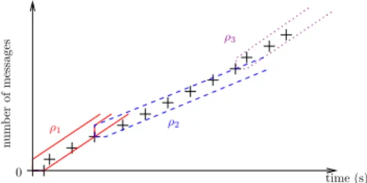
Example 4 Figure 3 introduces an example of message arrival dates and rates computed by the algorithm over the time. During the arrivals of 12 messages three rates are computed (ρ1, ρ2, ρ3).
ρ1 0 n um b er of messages ρ2 time (s) ρ3
Figure 3: Example time-window computed with the low profile behavior detection algorithm.
This method immediately returns for each studied flow a succession of burst indicators. We show (section 6) that these indicators vary considerably. However, these variations are not linear through out the experiment. Indeed, during several periods the arrival rates are almost stable while during others they are unstable, oscillating between low and high values. We believe that the different behaviors of alarm arrivals, showed by the burst indicators, highlight significant events on the network. Consequently, this approach has the great advantage to give an overview of the flow studied very quickly. Also, its application is very interesting because no expert is needed to interpret the result.
6
Experiments and results
In order to validate the proposed algorithm, we challenge our method to the real network issues of an operator, customer of Alcatel-Lucent Customer Services. Alcatel-Lucent Customer Services team has performed a deep proactive analysis of the network, relying on the network architecture and involving human expertise of technologies. We focus our analysis on two network elements (NE), designated by N E − A and N E − B, of the Optical Synchronous digital hierarchy (SDH), from retrieved alarms log over a one year time scale. This represents up to 200K alarms just for this technological slice of the network. Let us note that its full optical layer is composed of more than 62K elements that are able to generate alarms. Currently each element analyses the whole mass of information received by a traditional management method which is a hard task.
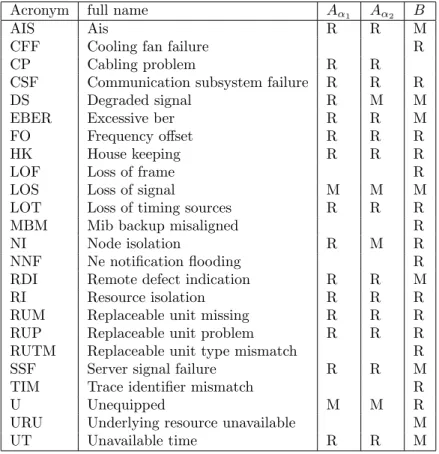
Acronym full name Aα1 Aα2 B
AIS Ais R R M
CFF Cooling fan failure R
CP Cabling problem R R
CSF Communication subsystem failure R R R
DS Degraded signal R M M
EBER Excessive ber R R M
FO Frequency offset R R R
HK House keeping R R R
LOF Loss of frame R
LOS Loss of signal M M M
LOT Loss of timing sources R R R
MBM Mib backup misaligned R
NI Node isolation R M R
NNF Ne notification flooding R
RDI Remote defect indication R R M
RI Resource isolation R R R
RUM Replaceable unit missing R R R RUP Replaceable unit problem R R R RUTM Replaceable unit type mismatch R
SSF Server signal failure R R M
TIM Trace identifier mismatch R
U Unequipped M M R
URU Underlying resource unavailable M
UT Unavailable time R R M
Table 1: List of the acronyms of the alarms.
To present significant results, the chosen network nodes are those identified by Alcatel-Lucent Customer Services to have failed several times during the studied year.
In this section, we first present the use-case we focus on and then analyze network elements N E −A and N E −B. Our objective is to prove that combining our low profile behavior detection algorithm and the new heuristic algorithm gives a precise analysis of the network behavior that concludes on the use case happening. To do so, we first use the low profile behavior detection algorithm. The idea is to obtain quickly a general idea of the network behavior. Then, we show that using the proposed algorithm creates set-patterns that highlights a succession of relevant alarms that gives meaningful information that permits to detect the use-case under study but not only.
10 Bouillard & Junier & Ronot
element N E − I, and fI
a the sub-flow of fI containing only occurrences of alarm a.
Table 1 lists the alarms found in the logs files studied. The three columns Aα1,Aα2 and B
represent the partition of the alarms between M and R respectively for N E − A with parameter α1, N E − A with parameter α2, and N E − B. An empty line means that the alarm is not present in the studied flow.
6.1
Use case description
In this article, we focus on a frequent issue: the laser failure of an optical SDH network element. Several alarms are symptomatic of such issue: LOS, AIS, LOF, TF (Transmitter failure), RUP, and RUM.
Occurrences of alarms LOS, LOF, and LOP (Loss of Pointer) render the whole signal unusable, which is replaced by an AIS consisting of continuous binary 1s. This produces occurrences of alarm AIS in every equipments downstream the fault: [ITU-T recommen-dation G.774 SDH - Management information model for the network element view];
The NE detecting a fault also sends an indication to the distant sending network element that an alarm has been raised. Some SDH elements also refer to a remote alarm indication at some levels in the hierarchy;
Alarms LOS, AIS, LOF can have many other triggers than a single laser component failure, whereas RUP, RUM and TF are the key to find the root cause of this use-case;
6.2
Study of a first network element
Let us focus on the analysis of the first node of interest called N E − A. It has generated 36K alarms of 17 types over the observed year.
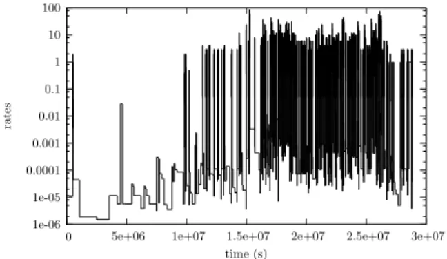
Figure 4 represents the variation of alarms arrival rates on the global flow of alarms fA com-puted with our low profile behavior detection algorithm (presented in section 5). One can observe
1e-06 1e-05 0.0001 0.001 0.01 0.1 1 10 100
0 5e+06 1e+07 1.5e+07 2e+07 2.5e+07 3e+07
rates
time (s)
Figure 4: Arrival rate of the global flow of alarms fA.
that rates computed are low and last a relatively long time up to 1.0 107s. Afterwards, rates range progressively becomes wider and rates variation amplifies. After 1.6 107s, the fluctuations reach their maximum and remain so until the end of the observation. From this curve, one can assume that a major problem occurs after 1.0 107s.
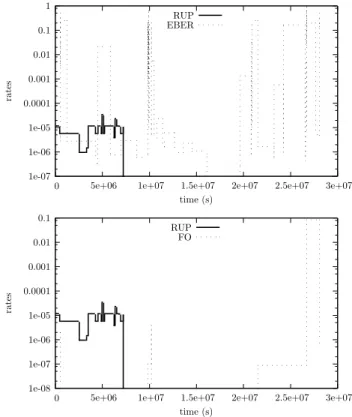
Let us now focus on the behavior of some alarms. Obviously we cannot represent the behavior of each alarm of the flow. Consequently, we decided to focus on alarm RUP as it is important for the use-case, but also EBER and FO. We will show later that those alarms give additional meaningful information about the health of N E − A.
The upper (resp. lower) part of Figure 5 represents computed rates for the sub-flows fA RU P and fA
EBER (resp. fRU PA and fF OA ). These graphics show that RUP occurs in fA only at the beginning of the flow, during the first 7.0 106
s. This assures the presence of the use-case. Alarm EBER appears all along the observation. However, one can detect bursts of arrivals: one around the arrivals of RUP (before 1.0 107s.) and an other one at the end of the year (after 2.0 107s.). Alarm FO only occurs three times. It shows a single burst at 5.0 105s. and an other one at 1.0 107s. Finally, more occurrences appear after 2.2 107s. Observing the arrivals of RUP one can suspect a correlation with EBER and FO.
Finally, one can observe that the instability observed on the global flow starts when RUP is not emitted any more. This might highlight that the use-case we focus on is not the major problem of this node.
1e-07 1e-06 1e-05 0.0001 0.001 0.01 0.1 1
0 5e+06 1e+07 1.5e+07 2e+07 2.5e+07 3e+07
rates time (s) RUP EBER 1e-08 1e-07 1e-06 1e-05 0.0001 0.001 0.01 0.1
0 5e+06 1e+07 1.5e+07 2e+07 2.5e+07 3e+07
rates
time (s) RUP
FO
Figure 5: Arrival rates of sub-flows fA
RU P, fEBERA and fF OA .
Let us now use our heuristic algorithm to obtain a refined analysis of N E − A. Choosing α1= 0.3 identifies two alarms as frequent: U and LOS. Their occurrences represent 97% of the total occurrences of alarms. The column Aα1 in Table 1 lists the partition of the alarms between M
and R.
Figure 6 represents the graph of set-patterns using α1= 0.3. We denote Group the set of alarms {DS, NI, CSF, EBER, RDI}, and the double slash bar represents the fact that the occurrence of the two set-patterns is separated by a long time period. This means that between
12 Bouillard & Junier & Ronot
the occurrence of these two set-patterns only alarms in M appear. Consequently, alarms relevant to a problem only occur at the beginning and the end of fA.
NI DS RUM CP HK DS FO SSF AIS CSF EBER RI RUP SSF RI AIS FO LOT Group Group SSF AIS UT FO RUM Group
Figure 6: Set-pattern graph with α1= 0.3.
Several observations can be made: first, the alarms that lead to a repair can be identified as RUP and RUM. Indeed, those alarms appear less frequently than the others. Using the small graph of the set-patterns obtained (that is acyclic), one can deduce the probable fault leading to RUM or RUP. It is also clear that HK and CP are related to RUM.
Secondly, RUP comes in a very large set-pattern, which may not be very meaningful. We can reduce the size of the pattern by setting α differently: for example, if we set α2 = 0.003 (about 10% of the remaining alarms after the suppression of U and LS), we add two alarms to M : M = {U, LOS, DS, NI} (column Aα2 in Table 1). Now |sp(f )| = 59. If we draw the interesting
part of the graph that concerns RUP and RUM, we obtain the graph of Figure 7. We can still observe the correlation between RUM, HK and CP. There might be a correlation there. We also notice that RUP mainly appears after the occurrence of SSF and CSF.
FO UT CSF EBER RDI EBER CSF RUP EBER CSF UT SSF AIS CSF EBER RUP RUP SSF RUM CP HK RUP RUM SSF RUP SSF EBER UT SSF AIS CSF EBER
Figure 7: Detail of the set-pattern graph with α2 = 0.003 during the occurrences of RUP and RUM.
We can now analyze precisely the results obtained with our methods. The observation of EBER and UT in the dependency graph shows that the issue is affecting a demodulator of the node. This is confirmed by the presence of FO is a set-pattern with UT and EBER. Alarm AIS has been set up avoiding any data on the channel. At the end, RUM and CP show that the element has been changed, such as they are directly followed by HK. Observing Figure 6 shows that, after a time, there is no more RUP or RUM emitted. Consequently, the problem has been fixed.
One can also remark that an other issue occurs after the substitution of the defect element and that it impacts much more N E − A (Figure 4). From Figure 6 we can deduce that the problem is linked to occurrences of alarms CSF and SSF, as they are present in almost each set-pattern. This indicates that a problem is coming from the optical link of the network element or from its neighbor connected through this link.
6.3
Study of a second network element
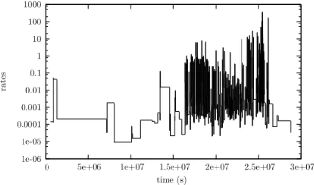
Let us now analyze N E − B which has generated 200K alarms of 23 types over the year. Figure 8 represents rates computed for flow fB. We can immediately observe that between 1.6 107
s. and 2.7 107
s. the arrivals intensify and vary considerably. More precisely, the instability starts slightly around 6.0 106
s. This can be explained by an earlier failure in the network that progressively impacts the network and drive its elements to generate much more alarms.
1e-06 1e-05 0.0001 0.001 0.01 0.1 1 10 100 1000
0 5e+06 1e+07 1.5e+07 2e+07 2.5e+07 3e+07
rates
time (s)
Figure 8: Arrival rate of the global flow of alarms fB.
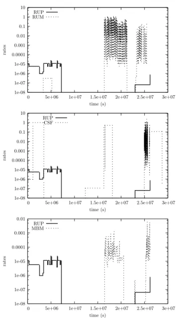
Let us now focus on some alarms known as important for the use-case studied: RUP and RUM. We also present the study of alarms MBM and CSF. We show later that these alarms give additional information about the network behavior. The higher part of Figure 9 represents sub-flows fB
RU P and fRU MB , the middle part shows fRU PB and fCSFB , finally the lower part represents fB
RU P and fM BMB .
Alarm RUP arrives in less than 6.5 106s. and at around 2.5 107s. It is interesting to observe that the first burst of RUP arrivals has exactly the same shape than in node N E − A. This tends to show that, before 6.5 106
s., N E − A and N E − B are observing the same pathology of the network. However, N E − B receives a second burst of RUP arrivals which is not the case for N E − A.
The top part of Figure 9 represents RUM and RUP. Alarm RUM appears slightly at the beginning, before 5.0 106
s. Then, it occurs between 1.6 107
and 2.1 107
s. and again between 2.3 107
and 2.6 107 s.
Alarm CSF is represented on the graphic in the middle of Figure 9. The computed rates indicate three bursts of arrivals. The first one arrives in less than 4.0 106
s. The second takes place between 1.3 107and 1.7 107s. Finally, the last one occurs after 2.5 107s.
Finally, the bottom part of the figure represents the behavior of MBM. One can observe that it occurs three times. One burst happens between 1.6 107 and 1.9 107s, a small burst arises at 2.2 107s, and the last burst arrives around 2.5 107s.
Note that the second arrival of RUP is accompanied with those of CSF, RUM, and MBM.
Let us now focus on the correlation study. We set α = 0.01 and we obtain M = {AIS, LS, SSF, DS, RDI, URU, EBER, UT} and |sp(f )| = 168, which is also a drastic decrease in the size of the alarms
repre-sentation.
Here again, the graph is too large to be drawn. However, a quick observation shows that the set of rare alarms is RUTM, CFF, HK, TIM and RI. Indeed, those alarms appear at most 10 times in fB. Also, RUP, U and LOF can be considered as rare alarms as they occur less than 65 times. Due to space restriction, we represent the most relevant parts of the graph. As previously, we intensely observe occurrences of RUP and RUM to highlight the use-case.
14 Bouillard & Junier & Ronot 1e-08 1e-07 1e-06 1e-05 0.0001 0.001 0.01 0.1 1 10
0 5e+06 1e+07 1.5e+07 2e+07 2.5e+07 3e+07
rates time (s) RUP RUM 1e-08 1e-07 1e-06 1e-05 0.0001 0.001 0.01 0.1 1 10
0 5e+06 1e+07 1.5e+07 2e+07 2.5e+07 3e+07
rates time (s) RUP CSF 1e-08 1e-07 1e-06 1e-05 0.0001 0.001 0.01
0 5e+06 1e+07 1.5e+07 2e+07 2.5e+07 3e+07
rates
time (s) RUP
MBM
Figure 9: Arrival rates of sub-flows fB
RU P, fRU MB , fCSFB and fM BMB .
Figure 10 represents a first pattern happening at the very beginning of the observation, where RUP appears for the first time (Figure 9). The presence of RUP and RUM in the set-patterns shows that the use-case we study effectively occurs. As previously, CSF is present with RUP. It is also the case for NI and U, that were major alarms in the previous case.
RUP NI CSF RUP NI CSF RUM RUP NI U NI CSF U RUM
Figure 10: Detail of the pattern-set sequences for Badra.
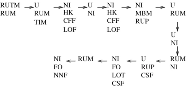
Figure 11 introduces a second pattern that is longer. It happens almost at the end of the observation, a short time before RUP appears for the second time. This figure is particularly interesting. Indeed, all the rare alarms (except RI) are represented in this pattern. Furthermore, one can observe that HK and CFF always occur together. There might be a correlation between those alarms. In addition, we can note the presence of CSF, NI, and MBM.
RUTM RUM U RUM TIM HK CFF NI LOF U NI HK CFF NI LOF U RUM NI MBM U NI RUM NI RUP U RUP CSF NI FO LOT CSF RUM NI FO NNF
Figure 11: Detail of the pattern-set sequences for Badra. We can now precisely analyze the results obtained by using our method.
First of all, we use once more our low profile detection behavior algorithm on fB
AIS. AIS is defined as major in this experiment, but it is also a good indicator of problems in a network. Studying its computed arrival rates, we deduce that AIS is always present in fB. This informs that N E − B is strongly disturbed during the whole experimentation.
The presence of RUP at the beginning of the observation shows that a NE is not performing properly and might fail. Also, the correlation with CSF indicates that the NE has communication problems. From Figure 9, we observe that RUP is not emitted during a long period of time after its first burst. We can conclude that the problem has been fixed.
The presence of RUP in the second pattern shows that another NE is failing (or the one that has already crashed). To obtain a better knowledge of the network behavior, the low profile detection behavior algorithm is used on major alarm EBER. It is interesting to observe that EBER appears only between 2.1 107 and 2.6 107s, which corresponds to the time period when RUM and RUP appear. The correlation between RUM, RUP and EBER indicates that a problem affects a laser demodulator.
Figure 11 points out others pathologies than the use-case studied. Indeed, we observe that CFF is correlated to HK. Alarm CFF indicates that the temperature of an element is above the tolerance threshold. The correlation of CFF and HK shows that several attempts have been performed to solve this problem. However, studying these two alarms shows that they appear a few times, which suggests that the first repairs haven’t worked. Finally, the presence of MBM and CSF highlights a communication problem with the controller card.
16 Bouillard & Junier & Ronot
These diagnostics have been easily refined and rooted by traditional means, using the pointed out alarm deep analysis. Our method avoids the use of filter in NMS and then the loss of the context in the issue diagnostic process.
Conclusion
This article presents a method to correlate alarms in a network. Our idea is based on the principle that due to the huge alarm variety, which progressively increases, most of them no longer refer to any critical problem. Consequently, we believe that a fault is highlighted by non-frequent alarms.
The method developed is realized in two steps. In a first time, we use as earlier work to give an overview of the network health. It is also useful to analyze the behavior of alarms detected as relevant. The second step uses the new algorithm introduced in this paper. It creates a dependency graph of sequences of alarms (set-patterns) from a studied flow. From this graph, rare alarms are extracted. They are those that might result from a critical problem. Focused on these alarms and small parts of the graph, we express hypotheses about the network health. Both algorithms used are very light in computing complexity and in memory usage.
Future work will include a proactive method that studies flows of alarms from every node of the network. It will aim at alerting the user as soon as possible on deviant behavior from the detected correlations.
References
[1] Alexandre Amaral, Bruno Zarpel˜ao, Leonardo de Souza Mendes, Joel Jos´e Puga Coelho Rodrigues, and Mario Lemes Proen¸ca. Inference of network anomaly propagation using spatio-temporal correlation. J. Network and Computer Applications, 2012, 35(6):1781–1792, 2012.
[2] Jean-Yves Le Boudec and Patrick Thiran. Network Calculus: A Theory of Deterministic Queuing Systems for the Internet, volume LNCS 2050. Springer-Verlag, 2001. revised version 4, May 10, 2004.
[3] Anne Bouillard, Aurore Junier, and Benoit Ronot. Hidden anomaly detection in telecommu-nication networks. In Conference on Network and Service Management, 2012 (CNSM’12), pages 82–90, 2012.
[4] Chen-Shang Chang. Performance Guarantees in Communication Networks. TNCS, Springer-Verlag, 2000.
[5] Tobias Chyssler, Stefan Burschka, Michael Semling, Tomas Lingvall, and Kalle Burbeck. Alarm reduction and correlation in intrusion detection systems. In Detection of Intrusions and Malware Vulnerability Assessment, 2004 (DIMVA’04), pages 9–24, 2004.
[6] Randall Davis, Howard E. Shrobe, Walter Hamscher, K¨aren Wieckert, Mark Shirley, and Steve Polit. Diagnosis based on description of structure and function. In Second National Conference on Artificial Intelligence, 1982 (AAAI, 1982), pages 137–142, 1982.
[7] Christophe Dousson and Vu Dtfdng. Discovering chronicles with numerical time constraints from alarm logs for monitoring dynamic systems. In Proceedings of the 16th International
Joint Conference on Artificial Intelligence, 1999 (IJCAI’99), pages 620–626. Morgan Kauf-mann Publishers, 1999.
[8] Eric Fabre, Albert Benveniste, Stefan Haar, Claude Jard, and Armen Aghasaryan. Algo-rithms for Distributed Fault Management in Telecommunications Networks. In Proceedings of the 11th International Conference on Telecommunications, 2004 (ICT’04), volume 3124, pages 820–825, Fortaleza, Brazil, Br´esil, 2004. Springer.
[9] Yang Fan. Improved correlation analysis and visualization of industrial alarm data. pages 12898–12903, August 2011.
[10] Thomas Guyet and Ren´e Quiniou. Mining temporal patterns with quantitative intervals. In Proceedings on the 4th International Workshop on Mining Complex Data, 2008 (ICDM’08) Workshop, page 10, Italie, 2008.
[11] Thomas Guyet and Ren´e Quiniou. Extracting temporal patterns from interval-based se-quences. In International Join Conference on Artificial Intelligence, 2011 (IJCAI’11), Barcelone, Espagne, Jul 2011.
[12] Bill Hollifield and Eddie Habibi. The Alarm Management Handbook: Seven Effective Meth-ods for Optimum Performance. Isa, 2007.
[13] Control Arts Inc. Alarm system engineering. In http://www.controlartsinc.com/Support/Publications.html, 2010.
[14] Gabriel Jakobson and Mark Weissman. Alarm correlation. IEEE Network 1993, 7(6):52–59, 1993.
[15] Irene Katzela and Mischa Schwartz. Schemes for fault identification in communication networks. IEEE/ACM Transactions on Networking, 1995, 3(6):753–764, December 1995. [16] Mario Lemes Proen¸ca, Bruno Zarpel˜ao, and Leonardo de Souza Mendes. Anomaly detection
for network servers using digital signature of network segment. In AICT/SAPIR/ELETE 2005, pages 290–295, 2005.
[17] Isabelle Rouvellou and George W. Hart. Automatic alarm correlation for fault identification. In International Conference on Computer Communications, 1995 (INFOCOM’95), pages 553–561, 1995.
[18] Arun Tangirala, Sirish Shah, and Nina Thornhill. Pscmap: A new tool for plant-wide oscillation detection. Journal of Process Control, 2005, 15:931–941, 2005.
[19] Tony White and Niall Ross. An architecture for an alarm correlation engine. In Object Technology, 1997, 1997.
[20] Fan Yang, S.L. Shah, and Deyun Xiao. Correlation analysis of alarm data and alarm limit design for industrial processes. In American Control Conference, 2010 (ACC’10), pages 5850–5855, 2010.
[21] Bruno Zarpel˜ao, Leonardo de Souza Mendes, Mario Lemes Proen¸ca, and Joel J. P. C. Rodrigues. Parameterized anomaly detection system with automatic configuration. In Global Communication Conference Exhibition and Industry Forum (GLOBECOM’09), pages 1–6, 2009.
RESEARCH CENTRE
RENNES – BRETAGNE ATLANTIQUE
Campus universitaire de Beaulieu 35042 Rennes Cedex
Publisher Inria
Domaine de Voluceau - Rocquencourt BP 105 - 78153 Le Chesnay Cedex inria.fr