Final report, research project INRS-Eau, Hydro-Québec*:
GREATLAKES
NET BASIN SUPPLY SIMULATION
BY A STOCHASTIC APPROACH Rapport scientifique no 362 Louis Mathier Laura Fagherazzi Jean-Claude Rassam Bernard Bobée November 1992 INRS-Eau Université du Québec C.P.7500 Sainte-Foy (Québec) GIV 4C7
Page
LIST OF TABLES ... iii
LIST OF FIGURES ... v
ACKNOWLEDGEMENTS ... 1
INTRODUCTION ... 3
1. Properties of the net basin supplies (NBS) ... 7
1. 1 Annual series ... 7
1.1.1 SeriaI correlation ... 8
1. 1.2 Cross-correlation ... 8
1.1.3 Frequency analysis and normality test ... l3 1.1.4 Run properties ... 18 1.1.5 Hurst coefficient ... 19 1.1.6 Spectral analysis ... 20 1.1.7 Homogeneity ... 22 1.2 Monthly series ...•... 29 1.2.1 Month-to-month correlation ... 29 1.2.2 Monthly.~ross-correlations ... 39
1.3 Properties to be explicitly preserved by simulation ... 40
2. Review of stochastic models and model selection ... 41
2.2 Description of the pre-selected models ... 43
2.2.1 Multivariate AR(1) model with shifting levels ... 44
2.2.2 Multivariate ARMA(1,1) model ... 46
2.2.3 SVD model ... 48
2.2.4 Data transformation ... 50
3. Samples simulation, validation procedures and final model selection ... 52
3.1 Samples simulation ... 52
3.2 Validation procedures ... 53
3.2.1 Validation of annual series: comparison ofhistorical and generated annual NBS ... 54
3.2.2 Validation ofmonthly NBS series: comparison ofhistorical and generated monthly NBS of Lake Ontario ... 62
3.2.3 Validation of quarter monthly levels: comparison ofhistorical and simulated level of Lake Ontario ... 68
3.3 Final model selection ... 75
4. NBS data generation ... 77
4.1 Simulation ... 77
4.2 Validation of the generated annual NBS ... 77
4.2.1 Basic annual statistics ... 78
4.2.2 Time series properties ... 78
4.2.3 Spatial properties ... 85
4.2.4 Frequential properties ... 86
5. CONCLUSION ... 91
REFERENCES ... 92
Table l.1: Table l.2: Table l.3: Table 1.4: Table l.5: Table l.6: Table 1.7: Table 2.1: Table 3.1: Table 3.2: Table 3.3: Table 3.4: Table 4.1: Table 4.2: Table 4.3: Table 4.4:
Basic statistics of annual NBS (tcfs) ... 7
Correlation coefficients between annual NBS of the four lakes ... 8
Significant lag-k cross-correlations between annual NBS for the four Lakes ... 13
Kolmogorov-Smirnov goodness-of-fit test ... 18
Maximum surplus run length (RL) and run volume (RS) ofhistorical data ... 19
Skewness coefficients of monthly NBS for the four lakes ... 34
Significant lag-O cross-correlations between monthly NBS for the four Lakes .. 39
Data transformation based on the highest Philliben correlation for annual and monthly NBS at aIl sites, 1 = normal, 2 = 2-parameter lognormal distribution, 3 = 3-parameter lognormal distribution, 4 = 3-parameter gamma distribution ... 51
Basic annual statistics and Hurst coefficient for Lake Erie ... 55
Annual cross-correlations ... 56
Surplus run length (RL) and run volume (RS) (Lake Erie) ... 62
Comparison of the three models ... 76
Basic statistical parameters ... 79
Hurst coefficients ... 84
Surplus run analysis (4-year running average) ... 85
Annual NBS lag-O cross-correlations between the four Lakes ... 86
Figure 1.1: Great Lakes - Saint Lawrence River Basin (from Yee et al. 1990) ... 4
Figure l.2 a: Lag-one to lag-24 correlogram for Lake Superior. ... 9
Figure l.2 b: Lag-one to lag-24 correlogram for Lake Michigan-Huron ... 10
Figure l.2 c: Lag-one to lag-24 correlogram for Lake Erie ... Il Figure l.2 d: Lag-one to lag-24 correlogram for Lake Ontario ... 12
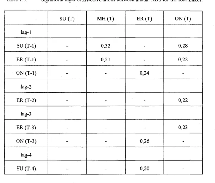
Figure l.3 a: Frequency plot of annual NBS using the Weibull plotting position formula on normal probability paper for Lake Superior. ... 14
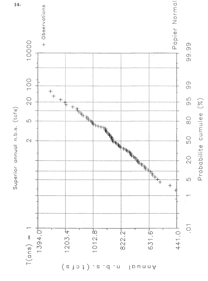
Figure l.3 b: Frequency plot of annual NBS using the Weibull plotting position formula on normal probability paper for Lake Michigan-Huron ... 15
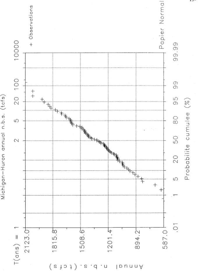
Figure l.3 c: Frequency plot of annual NBS using the Weibull plotting position formula on normal probability paper for Lake Erie. ... 16
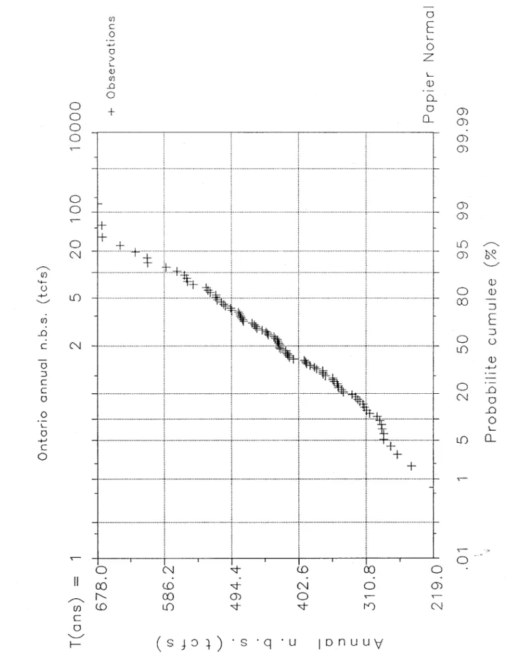
Figure l.3 d: Frequency plot of annual NBS using the Weibull plotting position formula on normal probability paper for Lake Ontario ... 17
Figure 1.4: Variance spectra of Great Lakes standardized series of annual NB S ... 21
Figure l.5 a: Annual net basin supply for Lake Superior ... 23
Figure l.5 b: Annual net basin supply for Lake Michigan-Huron ... 24
Figure 1.6 a: Annual net basin supply for Lake Erie ... 25
Figure l.6 b: Annual over basin precipitation for Lake Erie ... 26
Figure l. 7 a: Annual net basin supply for Lake Ontario ... 27
Figure 1. 7 b: Annual over basin precipitation for Lake Ontario ... 28
Figure 1.8 a: Mean and standard deviation ofmonthly NBS (tcfs) for Lake Superior ... 30
Figure 1.8 b: Mean and standard deviation ofmonthly NBS (tcfs) for Lake Michigan-Huron ... 31
Figure 1.8 c: Mean and standard deviation ofmonthly NBS (tcfs) for Lake Erie ... 32
Figure 1.8 d: Mean and standard deviation ofmonthly NBS (tcfs) for Lake Ontario ... 33
Figure 1.9 a: Lag-l to lag-3 month-to-month correlation coefficients for Lake Superior. ... 35
Figure 1.9 b: Lag-l to lag-3 month-to-month correlation coefficients for Lake Michigan-Huron ... 36
Figure 1.9 c: Lag-1 to lag-3 month-to-month correlation coefficients for Lake Erie ... 37
Figure 1.9 d: Lag-l to lag-3 month-to-month correlation coefficients for Lake Ontario ... 38
Figure 3.1: Correlogram ofannual NBS (Lake Erie) for a) SL, b) ARMA, and c) SVD ... 58
Figure 3.2: Frequency plot ofannual NBS (Lake Erie) for a) SL, b) ARMA, and c) SVD ... 59
Figure 3.3: Retum period (Weibull) ofannual NBS (Lake Erie) for a) SL, b) ARMA, and c) SVD ... 60
Figure 3.4: Mean ofmonthly NBS (Lake Ontario) for a) SL, b) ARMA, and c) SVD ... 64
Figure 3.5: Standard deviation of monthly NB S (Lake Ontario) for a) SL, b) ARMA, and c) SVD ... 65
Figure 3.6: Monthly NBS lag zero cross-correlations between Lake Erie and Lake Ontario for a) SL, b) ARMA, and c) SVD ... 66
Figure 3.8: Mean of quarter monthly levels (Lake Ontario) for a) SL, b) ARMA,
and c) SVD. . ... 69
Figure 3.9: Maximum of quarter monthly levels (Lake Ontario) for a) SL, b) ARMA, and c) SVD ... 70
Figure 3.10: Frequency plot of the sorted quarter monthly maximun annuallevel and min. max. and max. max. of simulated values (Lake Ontario) for a) SL, b) ARMA, and c) SVD ... 72
Figure 3.11: Global frequency plot of the sorted maximun quarter monthly annual level (Lake Ontario) for a) SL, b) ARMA, and c) SVD ... 73
Figure 3.12: Frequency plot with a retum period scale (Weibull) of the maximun quarter monthly annuallevel (Lake Ontario) for a) SL, b) ARMA, and c) SVD.74 Figure 4.1 a: Correlogram of annual NBS for Lake Superior ... 80
Figure 4.1 b: Correlogram of annual NBS for Lake Michigan-Huron ... 81
Figure 4.1 c: Correlogram of annual NBS for Lake Erie ... 82
Figure 4.1 d: Correlogram of annual NBS Lake Ontario ... 83
Figure 4.2 a: Annual NBS retum period (using the Weibull formula) for Lake Superior ... 87
Figure 4.2 b: Annual NBS retum period (using the Weibull formula) for Lake Michigan-Huron ... 88
Figure 4.2 c: Annual NBS retum period (using the Weibull formula) for Lake Erie ... 89
Figure 4.2 d: Annual NBS retum period (using the Weibull formula) for Lake Ontario ... 90
ACKNOWLEDGEMENTS
The present study was carried out by the Institut National de la Recherche Scientifique - Eau (INRS-Eau), and by Hydro-Québec Direction Production et Échange d'Énergie with guidance by, and interaction with an expert committee. We would like to thank the members of the committee
Dr. Bill Hogg of Environment Canada, Mr. Dave Rockwood of SSARR consultants,
Mr. Jean-Louis Bisson of Division Hydrométéorologie Hydro-Québec, Mr. Narut Kang of Groupe Équipement Hydro-Québec, Mr. Douglas Sparks of Groupe Équipement Hydro-Québec, Prof essor Michel Slivitzky of INRS-Eau, Prof essor Jose Salas of Colorado State University, and Dr. Frank Quinn of the Great Lakes Environmental Research Laboratory.
Other participants were Dr. Jan Grygier, consultant (California), Prof essor
v.T.v.
Nguyenof McGill University Montreal, Mr. David Fay of the Great Lakes Saint-Lawrence Office,
Mrs Deborah M. Lee of the Great Lakes Environmental Research Laboratory, and Mr. Jacques
Bourret Service Production of Hydro-Québec. We would like to stress the important input to this study by expert committee members Dr. Quinn, Prof essor Slivitzky, and Prof essor Salas who provided their assistance up to the very end.
We would like to thank the people who initiated and made possible this study, in particular Mr. Roger Larivière, previous head of Service Production, Hydro-Québec today retired and
Dr. Jean-Pierre Lardeau, head of Service Hydraulique, Hydro-Quebec as well as Mr. Gilles
j j j j j j j j j j j j j j j j j j j j j j j j j j j j j j j j j j j j j j j j j j j j j j j j j j j j j j j j j j j j j j j j j j j j j j j j j
INTRODUCTION
This final report presents the results of the stochastic approach used to simulate synthetic series of the Great Lakes net basin supply (NBS) for the Beauharnois-Les Cèdres extreme flood
study (Ras sam et al. 1992). A six months duration contract (DAC-91-ERE-342) was awarded to
INRS-Eau to analyze the historical records (90 years long) of net basin supply (NBS) of the Great Lakes Basin, review the literature on large-scale multivariate generation techniques and simulate 555 series of 90 years long of NBS on a monthly base. The study has been performed from november 1991 to april 1992 at INRS-Eau in collaboration whith Hydro-Québec.
The Net Basin Supply (NBS) series for Lakes Superior (SU), Michigan-Huron (MH), Erie (ER) and Ontario (ON) were used as the data base for modelling and data generation. Figure 1.1
shows a map of the Great Lakes - Saint Lawrence River Basin. In this study the NBS have been
computed as a residual of the water balance equation written as
where:
QI
is the connecting channel inflow00
is the connecting channel outflowD is the net diversion in or out of the lake
CU is the consumptive use
~S is the change in lake storage.
(la)
This definition of NBS is generally used for hydrological study of the Great Lakes Basin (IGLLB 1973). The NBS data have been validated and coordinated by the US Corps ofEngineers
and are provided by the Great Lakes Evironmental Research Laboratory (GLERL), Ann Arbor,
Michigan. A description of the Great Lakes system and NBS definition is provided by Yevjevich (1975).
The alternative method of computing NB S is the component method expressed as
( --, MINNESOTA ~::-~. r-_/ \ _./ J 1 DULUTH \ ( \--, \ /0.-WISCONSIN ILUNOIS Figure 1.1:
" \ ~GREAT LAKES DRAINAGE
\.. / 1 "'\ \ 'r ---> ~ / \ r, ./ PENN. SCALE
OTTAWA RIVER DRAINAGE BASIN
,,~., é~/
\ ('-"
j OUEBEC a 100 200 W ... êd a 100 300 Km ~S~~~~g;;;;~' 150 iIJ miles 50where:
P is the overlake precipitation
R is the runoff from the basin into the lake
E is the evaporation from the lake surface.
The differences in the procedures are discussed by Quinn and Guerra (l986). The significance of the differences is that, when evaluating management alternatives, it is necessary to evaluate past water supplies under current channel conditions. The use of equation (la) could therefore bias the computations by incorporating errors in connecting channel flow measurements due to measurement techniques or the computation ofregime changes. As noted by Quinn (1982), this could result in a considerable error in computing NBS prior to the current channel regimes.
Quinn (1982) shows that a 5 % error in either the Detroit or Niagara River flows would result in a
34 % error in the Lake Erie NBS computed by equation (la). A corresponding 5 % error in the precipitation, runoff, or evaporation terms in equation (lb) would result in a 4-5 % error in the Lake Erie NBS. Thus, while there is uncertainty in the evaluation of the components of equation (lb), the relative impacts are considerably less than in the case of the connecting channel flows. Therefore, it should be recognized that there are potentially large errors which could be introduced in the NBS computed for different channel regimes used in the study. One has to keep in mind that as far as water supply for the entire Great Lakes Basin are concerned the NBS data base computed by equation (la) is the best existing information that allows us to treat the problem.
In the first section ofthis report properties of the historical records ofNBS are presented for annual and monthly values. Description of the historical NBS is given in time, frequency and spectral domains. This analysis will be used for the selection of the properties to be explicitly preserved for the data generation. The second section presents a literature review of multivariate stochastic models. Section 3 describes the validation procedures and the final model selection. Three multivariate stochastic models were selected to generate annual and monthly NBS samples for the four lakes. For each model, the monthly NBS samples were used to simulate quarter monthly water level data at Lake Ontario. The three samples (annual NBS, monthly NBS, quarter monthly level) were used to validate the NBS and level data against historical records using several validation criteria. This phase is called the exploratory validation. Section 4 presents the final data simulation and validation of NBS for the Great Lakes. This phase is called the confirmatory validation. Finally, the conclusions of the study are presented in the last section.
1. Properties of the net basin supplies (NBS)
Properties of the NBS in the time, frequency and spectral domains are analyzed. The analysis of the basic data (historical NBS) considers both annual (long term) and monthly statistics. Annual statistics include: mean, standard deviation, skewness coefficient, seriaI correlogram, cross correlation, frequency analysis (using WeibuU plotting position), fUn properties and test of normality. Likewise, monthly statistics include mean, standard deviation, skewness coefficient, month-to-month correlations and monthly cross-correlations.
Besides the analysis of basic statistics, annual time series for aU sites are tested statisticaUy to detect possible shift and trend. Analysis also includes basin precipitation time series to see whether apparent concurrent shifts or trends are observed in both NBS and basin precipitation data. Apparent long-term persistence characteristics of the series are also discussed.
1.1 Annual series
Time series of annual NBS for the period 1900-1989 were obtained and analyzed statistically. The NBS series are analyzed by considering the calender year (January to December) while Hydro-Québec typically uses the year from October to September. This difference in the year definition does not make much difference for the purposes of the study. If not specified otherwise, the calender year definition is used in this report. Table 1.1 shows the basic statistics of annual NBS in thousand cubic feet per second (tcfs) for the four lakes.
Table 1.1: Basic statistics of annual NBS (tcfs).
MH
ER
ONmean 870,1 1344,3 236,4 430,1
standard-deviation 204,0 312,1 110,3 98,1
coefficient of 0,026 -0,052 0,093 0,471
1.1.1 SeriaI correlation
Figures 1.2a,b,c,d respectively show the lag-1 to lag-24 correlograms for the four Lakes. For Lake Superior and Lake Michigan-Huron the lag-1 correlation coefficients are low (respectively 0,16 and 0,19). For Lake Erie the lag-2 (r = 0,22) and lag-5 (r = 0,28) coefficients
are low but significant at a 5% level of significance. For Lake Ontario the lag-1 (r = 0,29), lag-2 (r
=
0,25), lag-3 (r=
0,22) and lag-four (r=
0,21) coefficients are also low but significant at the same level of significance.1.1.2 Cross-correlation
Table 1.2 gives the matrix of correlation coefficients between annual NBS of the four lakes.
Table 1.2: Correlation coefficients between annual NBS of the four lakes.
SU MH ER ON
SU 1,00
MH 0,54 1,00
ER 0,30 0,50 1,00
ON 0,27 0,62 0,66 1,00
In general the correlation structure shows a good spatial pattern (Fig. 1.1). Downstream from Lake Superior the correlation coefficients with other lakes are decreasing. Except for Michigan-Huron and Erie the correlations are always higher for two adjacent lakes. The correlations between neighboring lakes are higher going downstream or for smaller lakes.
.j.J C
•
• -4 U .-4...
...
•
o u E.timated Autocorr.lations Lake SupRrior 1 -1 r-+··· _ ... - , -8 6 18 16 la"Figure 1.2 a: Lag-one to lag-24 correlogram for Lake Superior.
~ c
•
...
u 1. 0.6 ~ 0 \.•
o u -0.6 -1. Figure l.2 b: o Lake Michigan-Huron 6 1.6 20 25 lag~ c
•
...
u...
'-'-•
o u 1 8.5 8 -8.5 -1 Figure 1.2 c: Estimated Autacarrelatians L8k .. Erie 8 5 18 15 28 25~ c
•
...
o 1 9.6 ·04 9\-•
o o -9.6 -1 Lak. Ontario 9 6 19 15 lagFigure 1.2 d: Lag-one to lag-24 correlogram for Lake Ontario.
1
i
1 1 1 1 ! 13-Table 1.3 lists only the significant lag-l to lag-4 cross-correlations at a 5% level of significance between annual NES for the four Lakes.Table 1.3: Significant lag-k cross-correlations between annual NES for the four Lakes.
SU(T) MH(T) ER(T) ON(T)
lag-l SU (T-l) - 0,32
-
0,28 ER (T-l)-
0,21 - 0,22 ON (T-l)-
- 0,24 -lag-2 ER (T-2)-
-
-
0,22 lag-3 ER (T-3)-
-
-
0,23 ON (T-3)-
-
0,26 -lag-4 SU (T-4)-
-
0,20-Up to lag-4 sorne of the correlations are significant at a 5% level of significance, but in general the coefficients are low.
1.1.3 Frequency analysis and normality test
Figures 1.3a,b,c,d respectivly show the frequency plots of annual NES using the Weibull plotting position formula on normal probability paper for Lakes Superior, Michigan-Huron, Erie and Ontario.
'+-ü (() ..0 c o :J c C o L o L V CL :J (J)
o
o
o
o
-+-' o > L Q) (f) -Do
+
_
...o
_
o _ ... .
+
· . ... , ... L ... -:-... [. ... ---... --.. --- · __ ···_··r···o
Z L Cl) 0.-o CL .. ... -. ...-:
~::~~l··+~;i::r::::r
•••••••••••••••••••••••
=
.=t-++:
.
· . l : : . ; : : N ... --trj11
---I---r---l---l--+
, -~ln
N
~
0b
.n
N N , - , -Il ~.
0 , - Nn
~ N 0 CD CD ~ ".-... (j) Cf)n
c , - , - , -0 '-....-/(SjJt) · S .
q
'U lonuuV 1-m (j) (j) (j) m m L.() (j)o
COo
L.()o
N L.()o
Cl) Cl) ::JE
::J () Cl) -+-' ..D o ..Do
L CLFigure 1.3 a: Frequency plot of annual NBS using the Weibull plotting position formula on normal probability paper for Lake Superior.
'+-ü (f) c o ::J C C o c o L ::J I 1 c o Q) ...c ü :2
o
o
o
o
.,--(f) c o +-' o > L <!) (f) ..cl o+
- ... ~... . ... , ... .o
_
o _ ... .
. .... i .. -- ... ----.4- .••.• -- •.•.•••••••••••••••.•••• ----j+
0E
L az
L Q) .-0.. 0 CL . ... -... + ... . . ...C-~
_ ... + ..
.++- .... L... ...
~
...
1... .....1...
...+-_ - . . . ...~.~
...~
... :. ... . ..~
... ."' - ...
....+~~,+,
... ... . , ... ...;
... f-N _ ... . . ... 1-: : . :~:::i-:l:~::l::!~r:::
i i i=tH-+
...•... ···1···,····t···· ... ; ... -_ ... 1"" ... ···l··· ...j ...
~-j!
1l
_ ... .i ... __ .. __ ...1
... __ ....
J ...
l ...
-1 1 1 ;.,--b:J
I.D
N
b
.;q- 0 Iln
. il).
CO . .,-- ..q-. 1'---0-J .,-- 0 0 (j) CO ~ (J) .,-- CO L() 0-J CO il) c 0-J .,-- .,-- ...--0 '-.../1-(SfJ+)
' S'q
'U lonuuV Ol Ol Ol Ol Ol Ol L() Olo
co
o
L()o
N L()o
Q) Q) :::JE
:::J () Q) 4-J ..û o ..û a L CLFigure 1.3 b: Frequency plot of annual NBS using the Weibull plotting position formula on
4 -Ü If) .D c o ::l C C o V L W -+-' 0 > L q) If) ..0 0 0
+
0 0 0 .,-------o
_
o --- _________ _
.,----+
o
Z --- --- ---~~
---~++j---···~'1f\i···
... .
U)···l''t
r ···
---~ ---1-~ --- --- ---0!q-
CD 1 ~ 1 (0 1 0 Il ~ . ~.
0 ()) f'--.. . (0 ~ f'--.. CD ()) (}) 0 .,----Cf) ~ 1") ~ .,---- .,----c 0 '---"" f-(s}J+)
. S .q
'U lonuu\jo
CDo
L{)o
~o
(!) Q) ::JE
::J Ü Q) -l-' ..0 o ..0o
L i lFigure 1.3 c: Frequency plot of annual NBS using the Weibull plotting position formula on normal probability paper for Lake Erie_
'+-ü (() .û c o :J C C o o L o +-' c
o
(f) c:: 0 0E
L +-' 0 > 0 Z '-V (f) -D L Q) .-0 0.. 0+
0 û. 0 0 0 , --... . .... ; ... , ... ! ... , ... ···ro
o _ ... .
···r "r~
0 + : N - .. ...+ . .. . ... " ... : ... _
... .
+
t
.
:
- ... : .+1€ ...
~1··· .. ·
... ~ . =t--:\if-
;
;
LO _ ... , ... ... ~ ... i ... ... , ... t-;:~
-I---l---!---j-+
...-o
Il CD ~I'- Cf) Ci) c o 1 1 N ~ . Ci) ~ CD <J) LO ~ (Sf:)~). S .
q
1 1 Ci) CD 0 N 0 <J) 0 , - , -~n
N 'U lonuu\j <J) <J) <J) <J) LO <J)o
CDo
LOo
No
Q) Q) :::JE
:::J o Q) +-' ...ûo
...ûo
L Û.Figure 1.3
cl:
Frequency plot of annual NBS using the Weibull plotting position formula on normal probability paper for Lake Ontario.1
1
Table 1.4 gives the result of the Kolmogorov-Smirnov goodness-of-fit test applied to the annual NBS series, where DN is the maximum absolute difference between the empirical distribution and the theoretical normal distribution with the parameters estimated from the observations. The P value is the probability of exceedance corresponding to the DN statistic obtained from the sample.
Table 1.4: Kolmogorov-Smirnov goodness-of-fit test.
SU MH
ER
ONDN statistic 0,085 0,062 0,087 0,056
P value 0,539 0,885 0,515 0,940
Based on a Kolmogorov-Smirnov goodness-of-fit test (Table 1.4) and on the normal probability plots (Fig. 1.3) it can be assumed that annual NBS for the four Lakes are normally-distributed.
1.1.4 Ruu properties
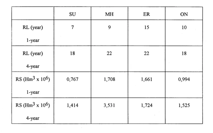
The run properties used in this study are defined according to Salas and Boes (1980). Let Xl,"" Xi,·.·, Xn, be a sample of size n. A positive value of Xi - c, where c is a constant threshold, is called a surplus. A consecutive sequence of exactly L surplus is called a surplus run of length L, and the sum of the surplus Xi -c over such a run is caUed the surplus run sumo The maximum surplus run length (RL) is the longest of aU the surplus run lengths in the sample. The largest surplus run sum in the sample is the maximum surplus run volume (RS). Table 1.5 gives the maximum surplus run length (RL) and the maximum surplus run volume (RS) of historical data for a truncation level (or constant threshold c) equal to the historical annual NBS mean. Both the traditional definition (one year) and the 4-year running average run criteria were used. In Table 1.5 RS is given in Hm3 x 106 units.
i
1
19-Table 1.5: Maximum surplus fUn length (RL) and fUn volume (RS) of historical data.
SU MH ER ON RL (year) 7 9 15 10 1-year RL (year) 18 22 22 18 4-year RS (Hm3 x 106) 0,767 1,708 1,661 0,994 1-year RS (Hm3 x 106) 1,414 3,531 1,724 1,525 4-year
Table 1.5 shows that the values of RL and RS are high, especially for Lakes Michigan-Huron and Erie.
1.1.5 Hurst coefficient
The Hurst coefficient (H) (Hurst 1951, Boes and Salas 1978) is used as an indicator of the persistence of a time series process. Persistence in streamflow is defined as a tendency for low flows to follow low flows and high flows to follow high flows. The Hurst phenomenon arises due to non-normality of the data, seriai correlation and nonstationarity in the underlying mean of the process. Asymptotically, for large normal independent series H = 0,5. Hurst has shown that the average value of H, observed for a large number of hydrological time series, is approximately 0,73.
The observed Hurst coefficients for the annual NBS of the four Lakes are:
0,647 for Lake Superior;
0,731 for Lake Michigan-Huron; 0,757 for Lake Erie, and;
0,752 for Lake Ontario.
The four sites have a high value of the Hurst coefficient, which indicates long-term persistence in annual NBS.
1.1.6 Spectral analysis
In the spectral analysis, the observed time series is considered as a random sample of a process in time that is made up of oscillations of aU possible frequencies. The variance spectrum partitions the variance into a number of intervals or bands of frequency (f). The spectral density is the amount of variance per interval of frequency. For a completely random series of uncorrelated numbers, the spectral density function (G(f) is constant and is termed white noise. This indicates that no frequency interval contains any more variance than any other frequency interval.
Figure 1.4 shows the variance spectra of Great Lakes standardized series ofannual NBS.
For the four Lakes, sorne frequencies contain more variance than the others (G(f) is not constant). For Lakes Superior, Michigan-Huron, Erie and Ontario there is a smaU-peak in the amplitude of the frequencies occuring respectively at f= 0,11, 0,16, 0,25 and 0,20. These peaks show that there is more variance in the standardized NBS for cycle periods of approximately 9 and 6 years for Lake Superior and Lake Michigan-Huron, and of 5 and 4 years for Lake Erie and Lake Ontario. For Lakes Erie and Ontario the cycle periods of the maximum variance spectra correspond to the observed lag-5 and lag-4 auto correlation coefficients. Thus, maximum variance spectra of the Great Lakes may indicate sorne long-term persistence in the annual NBS.
S
10°Cl
---""'----.... ....
Spectra of Great Lakes std series of annual NBS
,~Lake Superior -Lake Michigan . Lake Erie Lake Ontario -. --"':::"''---::0.--..: _ _ _ =-=. __ -"'---...::--10-1L-____ ~ ____ ~ ____ _ L _ _ _ _ ~ _ _ _ _ _ _ L _ _ _ _ ~ _ _ _ ~ _ _ _ _ L _ _ _ ~ _ _ _ _ ~
o
0.05 0.1 0.15 0.2 0.25 0.3 0.35DA
0045 0.5Frequency, f, in cycles per year
1.1. 7 Homogeneity
Figures 1.5a and 1.5b give the series of the annual NBS respectively for Lakes Superior and Michigan-Huron. The examination of figure 1.5 shows that the NBS for Lakes Superior and Michigan-Huron appear to be stationary. On the other hand, NBS series of Lake Erie (Fig. 1.6a) and Lake Ontario (Fig. 1.7a) show a positive jump or shift in the late sixties early seventies. Statistical tests have been performed to see whether these shifts are natural or man-made or a combination of both. Previous analysis of the data by the GLERL appear to indicate that such positive shifts may be due to similar shifts in the precipitation regime. It was decided to include in the analyses the series of annual over-basin precipitation. Figures 1.6b and 1.7b show the se series for Lakes Erie and Ontario. Visual examination offigures 1.6a, band 1.7a, b shows that there is a positive shift in both NB S and precipitation series. A bayesian approach was used to detect the most probable year of the occurence of the shift (Lee and Heghinian 1977, Bruneau and Rassam 1983) in the precipitation and NBS series.
The most significant change in the mean of precipitation and NBS series for Lakes Erie and Ontario occures simultaneously in or close to 1970. Since there is a concordance between the shifts in NBS and precipitation it can be assumed that the observed shifts in NBS are natural and that these shifts occured close to 1970. Based on this information a Mann-Whitney test of homogeneity (Mann and Whitney 1947) has been carried out on the four NBS series to see whether differences between the means oftwo subsamples (1900 to 1969 and 1970 to 1989) are significant. The results of the test of homogeneity for Lakes Superior and Michigan-Huron indicate that in both cases the two subsamples are homogenious at the 1 % level of significance. For Lakes Erie and Ontario there is a significant difference between the means at a 1 % level of significance. Thus, results of the bayesian approach and homogeneity test indicate that there is a shift in the annual NBS for Lake Erie and Lake Ontario. Based on this type of analysis it can be assumed that the shifts are an inherent property of the series which has to be taken into account in the stochastic model selection for the simulation.
Lake Superior
1400
1300
1200
1
-
1100
$ () ;t::.,1000
Cf)co
900
z
A1
1\
)
~
V\
~
V
lA~
mean
rn
:::J800
c
c
«
700
V
VV
N
\
1\
870
600
500
~
400
1900 1910 1920 1930 1940 1950 1960 1970 1980 1990
Year
Lake Michigan-Huron
2200
2000
1800
-
~1600
()...
...en
1400
ca
z
co
1200
::Jc
c
1000
«
800
~
/1vA~
f\
IAÂ
1
V
mean
V
\
('/V
Il1344
t1\
V600
400
1900 1910 1920 1930 1940 1950 1960 1970 1980 1990
Year
Lake Erie
500
mean
321
400
-
~300
() +-' ... (J)co
200
z
cu
::J c: c:100
~o
1\\
U\
/
1
1
1
V
1I~
1mean
A 1 1 A V (\/236
NV~
AI
lJ[;JV
212
1\
~
-100
1900 1910 1920 1930 1940 1950 1960 1970 1980 1990
Year
Lake Erie
120~---~110
f\
-
100
~
E
()~
{
~
'-'"c
JI
0rv
~
90
~~V\
~ a."u
\
ID1-80
a..
\ ~70
60+---~----~--~----~--~----~--~----~--~1900 1910 1920 1930 1940 1950 1960 1970 1980 1990
Year
Lake Ontario
750
700
mean
650
508
-
600
$u
+-'550
... CI)co
500
z
ctS :::J450
c
M
\
fv~.
nM
\1
\
~
mean
c
<l::400
350
300
\
\
\
430
V \f'-l
1V \
mean
V
~
408
~
\j
250
1900 1910 1920 1930 1940 1950 1960 1970 1980 1990
Year
Lake Ontario
115
110
105
-
E
100
u
...c
95
0~
...
90
"5..
u
ID....
85
a..80
75
70+---~----~--~----~----~--~----~--~--~1900 1910 1920 1930 1940 1950 1960 1970 1980 1990
Year
29-Results presented in the previous sections also indicate that long-term persistence is an important property of the series. This is shown by the high values of the fUn properties (Section 1.1.4), high values of the Hurst coefficient (Section 1.1.5) and peaks in the variance spectra (Section 1.1.6). It has also been noticed that sorne of these peaks coincide with high order auto correlation coefficients (Section 1.1.1).
Since unrealistic autocorrelations can result from the presence of a shift in the series (Salas
and Boes 1980, Salas etai. 1981), the validity ofthese statistics showing long-term persistence for
Lakes Erie and Ontario may be questionable. Due to the uncertainties induced in the series by the presence of a shift, the results can not be directly explained in term of persistence. Nevertheless, these characteristics (autocorrelation, RL, RS, Hurst coefficient, variance spectra) can be used to describe the data. Results of the normality test for Lakes Erie and Ontario (Section 1.1.3) may also be influenced by the non-homogeneity of the data induced by the shift (see Section 2.2.4).
On the other hand, for Lakes Superior and Michigan-Huron the results presented in the previous sections indicate that long-term persistence is an important characteristic of the series which has to be taken into account in the validation of the simulated data.
1.2 Monthly series
Time series of monthly NBS for the period 1900-1989 were obtained and analyzed statistically. Figures 1.8a,b,c,d and Table 1.6 respectivly show the mean, standard deviation and skewness coefficient of monthly NBS for the four lakes.
Mean peaks ofmonthly NBS occure in March on Lake Erie, in April on Lakes Ontario and Michigan-Huron, and in May on Lake Superior.
Most of the monthly series have a large coefficient of skewness, which indicate that the monthly observations are not normally-distributed. Thus, data transformation would probably be needed (see section 2.2.4).
1.2.1 Month-to-month correlation
Figures 1.9a,b,c,d show the lag-1 to lag-3 month-to-month correlation coefficients for the four lakes.
en IL (,) 210 170 130 9B .60 -30
L.k. Suparior Nat Sasin Supp1U 1900-1989
···f···t···I··· ... ~ ... ; ... ; ..•...
···t· __
···.;···j··· ... \ ...•... ~ ...••... 1. ••• . . . .... .L ...
L ... L ... _ .... ; ... ... L ... ···i···+···:···;=::::···t1~·AN···;···.: ... .. r+-
STAND OEV . _ . . . ~ . . . 04 • • U . . . ~ • • • • • • • __ . . . ~ . . . u . . + ... ~ ... .·r---
T··--···· .. [----:. __
.,-_.-
-.l·-·-;---r--·:-·-···t--·i---i---j---I·-····~_·----+-~ .. .. .. ~ : . . ;+--·---l---·J
---:cl<.::·:-~-l-::.=-~·:"--:.-~T~-~~F> <-+-~
' ! ; ~; "+-':-~"~F'~'~~-.. : .. .. ~ .. .. .. .. .. ~ .... : ... 04... . ... _ ... : ... ~ ... I ... 'u ... · ... , ... ; ... ,. ;
' ; ;
!
_·t·_··_·_··_-j···_···_···t···_····_···t··· ... 1 ... 1 ... 1.·_···_···i···]···l·_···_···t·_-_···L .. 1 2 :3 4 6 6 8 9 10 11 12 HONTH (~ANUARY=1)III Il. U >-.J a. a. :J III Z .... III <X ID 1-W Z
Monthlw Me~n and Stand~rd Ovvlatlon
Lake~ MlchlQan-Huron NBS 1900-1989 l ' , l ' 300
... : ... ; ... ; ... : ... ; ... ; ... ···;··· .. ····t···+··· ...
+
... ;. ... : ... .
: . : : 250 200 r···,···;··· ···,··1··· ... : ... , ...····:···,~···"MË·A·N···
.. :···· ... ; ....~
~
.
:
:
:
:
:
:
:. + _
STAND OEV ]~
... ... ~ ... ; .. ···7··· .. ···~···: ... ; ... .:.. ... ~ ... ~ ... .: ... ,.~
1j
150 • • • • • • • • • . . . • • : . . . h • • • • • • • ~ . . . : . . . ~ • • • • • • • • • • • • • • • • • • • ~ • • • • • • • • • • • • • • • • • • ~ . . . ~ . . . , H O , • • • { • • • • • • • • • • • • • • • • • • • : . . . : • • • • • • • • • • • • • • • • • • • • • • • • 100...
~... j ... : ...
~... ; ... ; ... : ...
1.. ...
j ... , ... ; ... .
. . 50*----f----+,
/ '...
... +
--+ - - -
-t ---
-+
/ ,/
+,
.. +_._. -
_.~:.
...
!
...
j •••.•.•••••....••• .L. ...~
..~
..~.+..~
..~
..~
..~
... ; ... : ... .:. ... . e ···t···t···;···:t···i.···· .. ···· .. ···;···\···t···!··· ... ' ....•...l ... . .
1 2 4 5 6 ï 8 9 10 11 12 MONTH (JANUARY=l)(f) IL (J >-.J a. a. :J (f) Z H (f) <I III
...
UJ Z 10a 75 5a 25 aMonthly Mean and Standard Deviation
Lak~ Erie Nes 1900-1989
...
~... ; ...
~...
~... ; ... ··f· .. ····,··· ..
~···~···.... ; ... .
1 1 -lj
MEAN .... ~ ... , ... ~ ... ,; .. , ... -.. '" ... ,--... ~ ... ; ... -... \., ... : ... " ... { ... ..~
:.+- STAND -..-
-... ~ ... ~ ... ~... . .. ~ ... ~ ... ~ ... ~ ... ~ ... ,.... . ..-t ---
.-+ - -
i--+
. - _ i-
-
-'-.
.... ; ... ; ... ~ ... L. ... ~ ... ; ... : ...j ... ; ... ' .. .
-25···t··· .. ···;· .. ··· ..
···l··· .. ·· ..
···f··· ..
···l··· .. ···: .. ··· .. ··· .. ··· ..i .. ·· .. ··· .. ··· .. f·· ... ··· .... · .. ·:···.· .... · .... · .... ;···· ...
1 ... : ... . 1 2 3 5 6 7 8 9 !oc 11 12 MONTH (JANUARY=l)... (JI IL o >-..J a. a. :::l (JI Z H (JI <I ID 1-UJ Z 100 80 60 40 20 o
Hcntnlu H.~n and Standard Deviation
Lake Ontario NBS 1900-1989 1 •• 1 • • 1 •
... '.. .... .. --.r ...
L . . . j . . _ - j .'t····'···-·l
, - - MEAN ...••..•••. J ...l ...
1. .. . • ~.. j . .. ··:··· .. ···~·· .. · .. ···1···· ···r··· ··· ... ·.·~··· .... ···t··· .. ···:-··· ... . j-+ - STAND DEV ; : . . . ... ·'j--··r···-·r···"-r
····-'·-···r····r--··r···'T-···r···l··-·-·r···T
t~·:~J~~~·l·~·~·T·~·:~t=~~+···i-
...
L-··~·j····J·:·~-td}
!
!
il-+'
+
' 1
1
.•• l. ••.• _ ... _ •• :._ ... _ ... l ... _ ... ~ ... ~ ... ~ ... ! ... .:. ... ~ ... : ... l .... _ ... i .... : : : : : : : : : : : : 1 2 :3 4 6 6 a 9 10 11 12 MONTH (~ANUARY=l)Figure 1.8 d:
Mean and standard deviation ofmonthly NBS (tcfs) for Lake Ontario.
33-Table 1.6: Skewness coefficients ofmonthly NBS for the four Iakes. SU MIl
ER
ON Jan 0,217 0,563 1,164 0,960 Feb 0,479 0,349 0,275 0,559 Mar 0,588 0,398 0,601 0,611 Apr 0,378 0,406 0,043 0,066 May 0,229 0,478 0,852 1,079 Jun 0,407 0,469 0,677 1,262 Jui 0,582 0,601 1,093 0,970 Aug 0,456 0,278 1,139 0,705 Sep 0,806 1,057 1,515 1,307 Oct 0,181 0,739 0,969 0,935 Nov 0,571 0,328 1,171 0,726 Dec -0,127 0,314 0,239 0,435Superior
month to month correlations
0 . 4 - r - - - , ,..---,
0.3
r(1,T)
r(2,T)
0.2~-7!---+----~-r----~---~~/
r(3,T)
/_
0.1
...
.. ,! \,,/~.! /""\' ....
\\\ / / ~~-
'-o ___
---.;'\l ___ ._._._ \ ! \ 1 \. i-0.1
\j -0.2r---~ -0.3+---~--~--~----~--~--~--~----~--~--~--~1
Oct
2
3
4
Jan
5
6 7 8
T (month)
9
10
11
Jun
Figure 1,9 a: Lag-1 to lag-3 month-to-month correlation coefficients for Lake Superior.
12
-...
~
-
:1..Michigan-Huron
month ta manth lag k correlations
0.5
004
r(1,T)
0.3
r(2,T)
0.2
,: "', ... /" ./\
\.r(3,T)
0.1
0
\
/~/'Y//"\0(~
/ / / _ _ .M. _ _ _ _ _ _ _ _ _ \\:~~~::~>?:~:.';/ _________ \ ",/
.... ' ... j~-0.1
-0.2
-0.3+---~--~--~--~----~--~--~--~--~--~--~1
Oct
2
3
4
Jan
5
6 7 8
T (month)
9
10
11
Jun
12
Sep
Figure 1.9 b: Lag-l to lag-3 month-to-month correlation coefficients for Lake Michigan-Huron.
Erie month to month lag k correlations
0 . 5 . - - - , ,---,0.4
critical values at 5%
0.3
0.2-1--~--f---!----":---\--+---f--,.~--.... -... -... - \ - - - + - 1 -1- /C
0.1 ... ,//'
~//
Jo.. ...• / / .••o
.---~---!
!-0.1
:. 1\ : ../
\.\
!
\.
: ../
/
-0.2r---\+\~!---~
\; -0.3+---~--~--~----~--~--~--~----~--~--~--~r(1,T)
r(2,T)
r(3,T)
1
2
Oct
3 4 5 6 7
8
Jan
T (month)
9
10
11
Jun
12
Sep
-
lo...0.7
0.6
0.5
0.4
0.3
0.2
0.1
o
-0.1
Ontario
month to month lag k correlations
critical values at
5%
... / ... , .. ~. ... ,... . .... ,...;! \ ... """'" .../~
...• '~" .../'''--~':::'
..
... ···f···....
..,/
....
I . _ _ _ _ _ ;.., _ _ _ .~~ i .•.•• ..-/ - - - 1 .,..- .~--r_---0.2~---~ -0.3+---~--~--~--~----~--~--~--~--~--~--~r(1 , T)
r(2,T)
r(3,T)
1
2
3
4
Oct
Jan
5
6 7 8
T (month)
9
10
11
Jun
12
Sep
39-In general, the month-to-month coefficients of correlation are low. For lag-1 and 2, the highest correlations are between autumn months, followed by spring and summer months. The lowest correlations are between winter months. AImost none of the lag-3 correlations are significant.
1.2.2 Monthly cross-correlations
Table 1.7 gives the significant lag-O cross-correlations at a 5% level of significance between monthly NBS for the four Lakes.
Table 1.7: Significant lag-O cross-correlations between monthly NBS for the four Lakes.
SU-MH SU-ER SU-ON MH-ER MH-ON ER-ON
Jan 0,29 - - 0,54 0,60 0,77 Feb 0,45 0,30 0,34 0,60 0,72 0,746 Mar 0,69 0,40 0,59 0,57 0,71 0,66 Apr 0,46
-
-
0,40 0,48 0,49 May 0,41-
-
0,51 0,64 0,73 Iun 0,56 0,21 0,33 0,52 0,54 0,54 Jul 0,34-
-
0,43 0,60 0,49 Aug 0,51-
0,25 0,48 0,43 0,36 Sep 0,52 0,27-
0,48 0,52 0,78 Oct 0,46-
0,21 0,59 0,41 0,67 Nov 0,57 0,39 0,25 0,52 0,52 0,75 Dec 0,59 0,42 0,40 0,58 0,61 0,74In general the correlation structure of monthly NBS shows a similar spatial pattern as the one observed for annual NBS (Table 1.2). As we go downstream from Lake Superior (Fig. 1.1) the correlation coefficients with other lakes decreases for each month. The highest correlations occure between Lakes Erie and Ontario. The lowest correlations between sites are in summer months.
1.3 Properties to be explicitly preserved by simulation
The examination of the statistical characteristics of historical annual and monthly NBS are used to select the properties to be explicitly preserved by the simulation.
In brief, it has been shown (section 1.1. 7) that the annual series of Lakes Superior and Michigan-Huron are stationary. Likewise, annual NBS series for Lakes Erie and Ontario show a significant shift in 1970. SeriaI correlations are low but significant, showing a complex dependance structure for Lakes Erie and Ontario (section 1.1.1) that may be induced by the observed shift in the series. The cross-correlations, ranging from 0,27 to 0,66, indicate that the spatial structure is
also important (section 1.1.2). The analysis of surplus run properties (section LIA), Hurst
coefficient (section 1.1.5) and spectral analysis (section 1.1.6) show sorne persistence in the series.
On the other hand, series of monthly NBS (section l.2) show large skewness and important seasonal variations of the mean, standard deviation and coefficients of correlation, which are in generallow but significant at a 5% level of significance.
Given these characteristics of NBS series and, given that this study relates to extreme events, more attention should be payed to reproduce properties at the annual time scale than at the monthly time scale. The analysis of the correlograms, run properties, Hurst coefficients and variance spectra clearly show the long-term persistence of the annual series. For Lakes Erie and Ontario, such complex dependence structure may be the result of the apparent shifts in the annual NBS series. Thus, emphasis will be placed on annual properties, although monthly properties will be considered as weIl.
The properties to be preserved or explicitly modeled are:
cross-correlation of order zero (spatial relationship);
seriaI correlation as shown in historical records (temporal relationship and persistence); upward shifts for Lakes Erie and Ontario;
mean and standard deviation;
basic properties ofmonthly series (monthly mean and standard deviation).
Sorne other implicit properties will be checked through validation criteria. Since previous studies on the Great Lakes Basin (see for example Loucks 1989) have suggested that certain models may not be able to reproduce observed historical Lake levels, even if the NBS are adequately generated, the analysis of the data would also includes properties of historical and simulated Lake levels provided by the GLERL (see section 3).
2. Review of stochastic models and model selection
The purpose of this section is to review and evaluate the models available in computer program form for stochastic generation of monthly NBS at several sites.
The literature on stochastic hydrology includes several univariate models. The autoregressive (AR) type of models are by far the most widely used in hydrology. Descriptions of univariate AR models applied in hydrology are given by Salas et al. (1980) and Fiering and Jackson (1971). Univariate models can be classified in three classes:
Autoregressive model, AR(p), where p den otes the order of the AR term;
Autoregressive Moving Average model, ARMA(p,q), where p and q denote the orders of the AR and MA terms;
Autoregressive Integrated Moving Average model, ARIMA(p,d,q), where d denotes the differencing component of the model and p and q are as defined before.
These models in their univariate form do not take into account spatial correlations between sites. They are not directly useful for multivariate modelling although, in certain modelling strategies they can be quite useful.
2.1 Multivariate models
The principal aims of multivariate models is to take into account the cross-correlation between sites. Multivariate AR and ARMA models can be constructed by fitting univariate models to each of the stations under study independently and then modelling the spatial correlation through the residuals. Generally, only the lag-O cross-correlation is considered by restricting the
parameters matrix of the model to be diagonal (Salas et al. 1980). These models are referred to as
contemporaneous such as the CARMA mode!. Review of multivariate models can be found in Salas et al. (1985), Stedinger et al. (1985a), Grygier and Stedinger (1990) and C.E.A. (1990).
Sorne theoretical aspects of multivariate models are discussed by Fiering (1964), Matalas (1967) and Bernier (1971).
Multivariate models can be classified in direct modelling approach and indirect modelling approach (Grygier and Stedinger 1988, C.E.A. 1990). Direct modelling is used to build the model directly based on the monthly time series. In the indirect approach the annual series are first generated and then the annual values are disaggregated into monthly or smaller time units.
A number of data generation studies has been made related to streamflow simulation (Young
and Pisano 1968, Srikanthan et al. 1983, 1984, Nathan et al. 1989, Salas and Abdelmohsen 1991).
Studies performed by Megerian and Pentland (1968), IGLLB (1973), Yevjevich (1975) and Loucks (1989) include simulation of the Great Lakes NBS. The latter studies have been performed using the direct approach. Generally, monthly NBS statistical properties are weIl reproduced by the direct approach. Unfortunately, the direct approach usually fail to adequately reproduce statistical properties and persistence of annual NBS (Grygier and Stedinger 1988). To preserve the long-term persistence characteristics observed in the annual NBS, a special attention will be payed to the indirect modelling approach. However, the direct approach wouJd also be considered as a back-up mode!.
A condensed disaggregation procedure proposed by Grygier and Stedinger (1988) has been choosen for the indirect approach. Multivariate step disaggregation (Santos and Salas 1991) is an alternative but the computer program was not available at the time of this study. Likewise the LAST model (Lane 1979, Lane and Fervert 1988) is an other alternative but the Grygier and Stedinger model is a more recent one allowing automatic selection of data transformation. Three reasons justify the choice of the Grigier and Stedinger (1988) model:
1) the complete procedure (including data transformation) is available in computer form in the SPlGOT Synthetic Streamflow Generation Software Package (Grygier and Stedinger 1990, 1991);
2) the Grygier and Stedinger (1990, 1991) condensed procedure reduces the number of parameters to be estimated (Grygier and Stedinger 1988) in comparison with other models like the Valencia-Schaake model (Valencia and Schaake 1973), LAST model (Lane 1979, Lane and Fervert 1988), and the Generalized SPC model (Stedinger et al.
1985b);
3) the procedure can explicitly reproduce the correlations between monthly and annual flows, the correlations between consecutive monthly flows, and the cross-correlations at different sites (Grygier and Stedinger 1990), although it cannot reproduce the correlation of the last season of the previous year with the first season of the current year.
The direct approach will be considered using a monthly-annual Singular Value Decomposition model (SVD) (Cavadias 1985), which is based on the principal component analysis (Fiering 1964, IGLLB 1973). The SVD model software is not available but it is relatively easy to code using available statistical packages. The SVD model has the main advantage of explicitly taking into account aIl the correlation structures of the data set in time and space.
2.2 Description of the pre-selected models
The model used to generate NBS should capture the important statistics of the record data. Since the multivariate AR(l) model available in SPlGOT may not be able to reproduce persistence, run characteristics and shifts in historical records, the use of alternative models are considered. Based on theoretical considerations, three models are selected for samples simulation. These models are described in the following sections. The choice of one model for the final simulation will be based on the results of an exploratory validation of generated samples (see section 3).
F or the indirect approach, two different procedures are used to reproduce the shifts at the annual time scale. The first procedure is built to directly introduce the shifts in the generated sequences of annual NBS using a multivariate AR(l) model with shifting levels. This procedure is based on the idea of shifting level modelling of hydrologic series proposed by Boes and Salas (1978), Salas and Boes (1980) and Salas et al. (1981). The second procedure will try to fit the general shape of the observed correlograms (Fig. 1.2) using a multivariate ARMA(1, 1) model. In both cases, the generated annual NBS will be disaggregated into monthly NBS.
For the direct approach, it will be assumed that the correlation structures of the monthly-annual data vectors, which are explicitly preserved using the SVD model, will be able to implicitly reproduce the shifts and other characteristics observed in the historical records.
2.2.1 Multivariate AR(I) model with shifting levels
In this model two sets of parameters of a multivariate AR( 1) model are estimated from the two parts of the historical records (first 70 years, last 20 years). To generate the annual NBS, SPIGOT will use one model for a certain time, then switch to the other and so on. The time spent at either level is taken from a geometric distribution. Parameter of the geometric distribution is set by the user to give average length of time to stay at each level over the whole generated sequences in the same proportion as the one observed in the historical records (in our case 70/20). The geometric distribution is used here as a mixing pro cess only, and no attempt is made to say that the duration of the observed shifts in annual NBS are geometrically-distributed. The second step in the data generation uses a multivariate annual to monthly disaggregation model to generate monthly NBS at the four sites.
A complete description of the stage disaggregation sheme used in this project is given in the SPIGOT Technical Description, Version 2.6 (Grygier and Stedinger 1990) and will not be repeted here. In the SPIGOT Technical Description report:
• the methodology of the Scheme III - Multivariate Annual Flow Generation and
Disaggregation is presented in page 13;
• Section 3.6 (page 23) gives the general description of the Multivariate Annual-Monthly
Model;
• Section 3.3 (page 19) gives the Multivariate Autoregressive Model used to generate
normally-distributed annual flow vectors (equa. 2*);
A procedure added to SPlGOT by Jan Grygier to generate random variates from the geometric distribution is described in the following section.
Generating random variates from the geometric distribution
We want to generate random variate Ni representing the length of a series at one level in the
shifting levels model, with Jl(N)
=
l/p=
20 or 70 years as an example.The geometric distribution has:
p[
N > n] = (1-p)n (2)P[N
=n]
= p(1- py-1 (3)We will generate variates from the uniform distribution D(O, 1) and then transform them.
The uniform distribution has:
p[
x>
x] =1-x (4)We want a transformation N = g(x) so that:
p[
N>
n]
=p[
X>
x]
(5)where n = g(x). Thus,
n
log(1-
p)
= log(1-
x)
(6) n = log(1-
x) / log(1-
p)
=g(
x )To get geometrically-distributed variates, we take samples from the U(O, 1) distribution and apply the transformation g to them.
Because (I-x) is distributed exactly the same as x when x cornes from U(O, 1) the SPlGOT program just uses
g(x)
= (logx)/log
(1-
p)
(7)In the current implementation SPIGOT asks the user to input the average length of time to stay at each level for the generation. In output, SPlGOT gives the time duration of each generated sequence and the average time spent at each level for the whole generation.
2.2.2 Multivariate ARMA(l,l) model
Autoregressive Moving Average time series models have proven to be a flexible tool for use in water resources planning. The ARMA(1,l) model, in particular, has a physically reasonable correlation structure which can reflect the long-term persistence observed in sorne geophysical
time series. It has been showed that persistence may result either from long memory in hydraulic
processes (Mandelbrot and Wallis 1968), or from shifts in the mean ofthese pro cesses related to climatic changes (Boes and Salas 1978). The ARMA(I, 1) structure may be considered compatible with either explanations that have been advanced.
The general multivariate ARMA(1, 1) model may be written
(8)
where Xt is an
rh
x 1 vector of normally-distributed flow residuals (zero mean) in period t with covariance matrix Sa,Vt is an m x 1 vector of time-independent normally-distributed random fluctuations with covariance matrix G,
Salas et al. (1980) and Loucks et al. (1981) have suggested that <1> and
e
be taken as diagonal matrices. Then the elements of each matrix are essentially the parameters of univariate ARMA(1,I) models fitted to the flows at each site (contemporaneous ARMA or CARMA model). This method has the advantage that each site is described with weIl known properties and that the multisite model is hydrologically reasonable. With the assumption of diagonality for <1> ande,
the model fitting pro cess is performed in two independent steps:1) estimation of <1> and
e;
2) estimation of the G matrix.The MATLAB, IDENT procedure (MATLAB 1990) was used to estimate the parameters <1>
and
e
for Lakes Superior, Michigan-Huron and Ontario. For Lakes Superior and Michigan-Huron,the parameter
e
of the MA process is not significant, which simply gives an AR(1) model with parameter <1>.For Lake Erie, due to the shape of the auto correlation function (Fig. 1.2) we could not obtain good estimates of the parameters <1> and
e.
To avoid this problem we simulate several autocorrelation functions for different values of <1> ande
(Salas et al. 1980). We choose the set of parameters which gives the best fit of the observed correlogram as a whole. The validity of this procedure will be checked a posteriori through the validation criteria.When the parameters <1> and
e
are estimated, Vt in Equation (8) can be aigebraically derived. T 0 arrive at white noise residuals, a model of the form(9)
may be used, where B is an m x m matrix of coefficients and et is an m x 1 vector of residuals with mean zero and variance one, which are uncorrelated in time and space.
In regard to the estimation of the covarIance of the residuals (matrix G) for the
CARMA(1, 1) model, Stedinger et al. (1985a) have recommended the following estimator
(10)
where
(soL
is the ij th element ofSo
the lag zero cross-covariance ofXt. Then, the matrix BIj
of equation (9) is given by solving
BB'=G (11)
In the current implementation SPI GOT cannot estimate the parameters for a general ARMA model, but it can generate ARMA(1,l) annual flows if the user puts the right parameters in the parameters file using estimated <l> and
e
and equations (9), (10) and (11). For this model we areusing the same SPIGOT disaggregation procedure as the one described in section 2.2.1.
2.2.3 SVD model
The multivariate simulation method proposed in the present study is based on the singular
value decomposition (SVD) theorem (Cavadias 1985). Consider the N xp data matrix X, and let r
be the rank of X. The singular decomposition ofa matrix X can be written as follows:
X=VD1
/2U' (12)
in which V is an N x r matrix of eigenvectors of XX'; D is a r x r diagonal matrix of the positive eigenvalues of XX'; and U is ap x r matrix of the eigenvectors of X' X.
Let Xs be the standardized matrix of X, that is, each colurnn of Xs has zero mean and unit variance. On the basis of equation (12), the matrix Ys of the standardized principal components of Xs is given by
v
= X UD-1/2s s (13)
Note that the colums of Ys are orthonormal, that is
v..'v..
=
l, and hence they can be generated independently following the distribution function of each colurnn of Y s.Equations (12) and (13) provide the basis for the generation ofmonthly and annual NBS for the four Lakes considered. More specifically, the steps in the calculation of the simulated data matrix
X
are as follows:1. Transform the observed data matrix X, where N represents the number of years of observation; and p = 52 indicates that for each of the four sites there are 13 data colurnns, into a normal data matrix X* using a three-parameter lognormal transformation.
2. Apply the first-order autoregressive models to the data matrix X*, and let E be the matrix of the residuals.
3. Compute the standardized matrix Es.
4. Compute the correlation matrix REs from Es, and its associated eigenvalue and eigenvector matrices D and U respectively.
5. Compute the principal component matrix Ys using equation (13).
6. Generate the matrix
t:
of random numbers following the probability distributions of thecolurnns of Ys.
7. Compute the standardized matrix Ys 1 from Y s' its corresponding correlation matrix Rys 1 and its associated eigenvalue and eigenvector matrices, UYsl and DYsl> respectively.