Development of a toolbox for assessment of aquatic habitat impacted by peat harvesting.

(1)

Record Number: 21490

Author, Monographic: St-Hilaire, A.//Courtenay, S. C.//Boghen, A. D.//Bobée, B.//Koutitonsky, V. Author Role:

Title, Monographic: Development of a toolbox for assessment of aquatic habitat impacted by peat harvesting Translated Title:

Reprint Status: Edition:

Author, Subsidiary: Author Role:

Place of Publication: Québec Publisher Name: INRS-Eau Date of Publication: 2001

Original Publication Date: Mars 2001 Volume Identification:

Extent of Work: iv, 37 Packaging Method: pages Series Editor:

Series Editor Role:

Series Title: INRS-Eau, rapport de recherche Series Volume ID: 587

Location/URL:

ISBN: 2-89146-454-0

Notes: Rapport annuel 2000-2001

Abstract:

Call Number: R000587

(2)

Development of a toolbox for

assessment of aquatic habitat

impacted by peat harvesting

(3)

Development of a toolbox for assessment of aquatic

habitat impacted by peat harvesting

By

André St-Hilaire

Simon C. Courtenay

Andrew D. Boghen

Bernard Bobée

Vladimir Koutitonsky

March2001

Research Report R-587

(4)

LIST OF TABLES

Table 1. Discharge statistics, station 01 B8001 (Coal Branch at Beersville) ... 16

Table 2. Chi squared (X2) tests for the four distribution functions tested to fit the flood

data from station 01 B8001 (Coal Branch) ... ~ ...•...•... 16

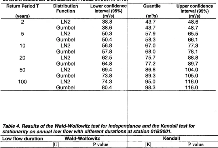
Table 3. Flood frequency analysis of Coal Branch flow data (station 01 B8001) ) using different statistical distributions. Floods shown in m3_{/s ...•...•...•....}₁₇

Table 4. Results of the Wald-Wolfowitz test for independance and the Kendall test for stationarity on annuallow flow with different durations at station

01B8001 ... 17

Table 5. Chi squared (X2) tests for the four distribution functions tested to fit the low

flow data from station 01 B8001 (Coal Branch) ... 18

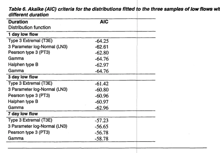
Table 6. Akaike (AIC) criteria for the distributions fitted to the three samples of low

flows with different duration ... 1:8

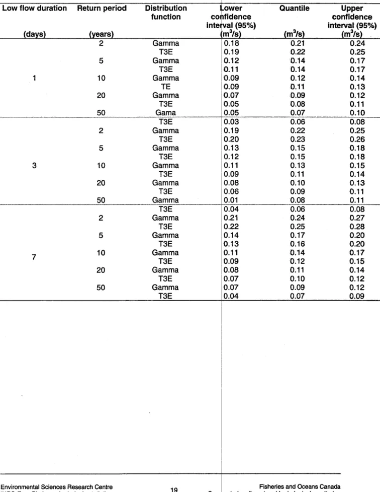
Table 7. Low-flow Frequency analysis of Coal Branch (8tation 0188001) using

different statistical distributions. Flows shown in m3/s ... 19

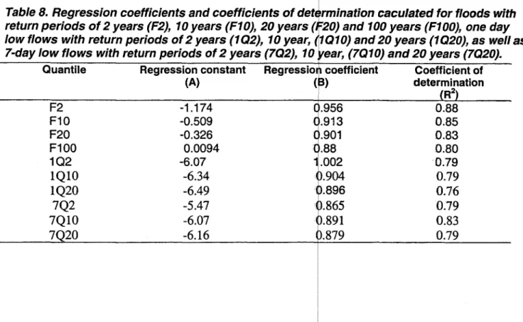
Table 8. Regression coefficients and coefficients of determination caculated for floods with return periods of 2 years (F2), 10 years (F1 0),20 years (F20) and 100 years (F100), one day low flows with return periods of 2 years (102), 10 year, (1010) and 20 years (1020), as weil as 7-day low flows with

return periods of 2 years (7Q2), 10 year, (7010) and 20 years (7020) ... 20

Table 9. Flood and low flows (m3/s) for sub-basins of the Richibucto watershed,

evaluated using equation 5 (regression between area and quanti/es) ..•...• 20

Environmental Sciences Research Centre INRS·Eau, Chaire en hydrologie statistique

ii

(6)

LIST OF FIGURES

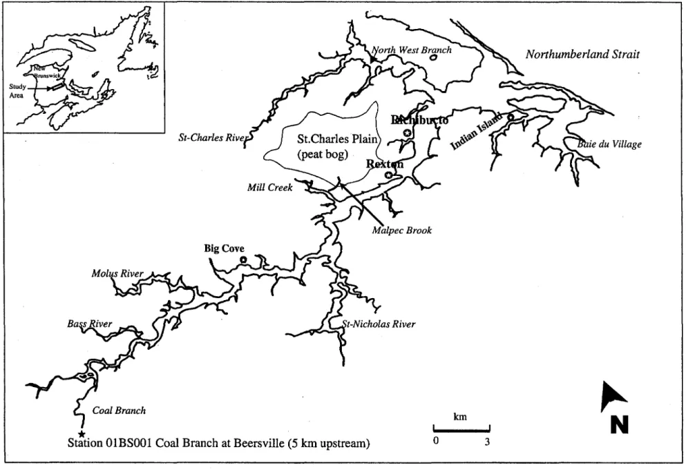
Figure 1. Map of the Richibucto area, showing Malpec Brook ... 21 Figure 2. Comparison of Logmormal (LN2) and Type 1 Extreme (Gumbel) distribution

functions with annual flood observations ... 22 Figure 3. Regression between two year flood discharge (F2) and drainage area (from

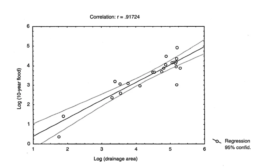
El Jabi et al. 1994) ... 23 Figure 4. Regression between 10 year flood discharge (F10) and drainage area (from

El Jabi et al. 1994) ... 24 Figure 5. Regression between 20 year flood discharge (F20) and drainage area (from

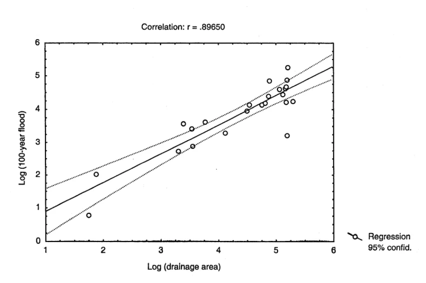
El Jabi et al. 1994) ... 25 Figure 6. Regression between 100 year flood discharge (F100) and drainage area

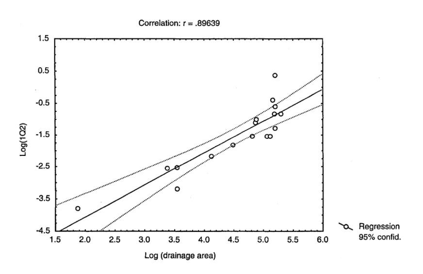
(from El Jabi et al. 1994) ... 26 Figure 7. Regression between two year low flow with a one-day duration (102) and

drainage area (from J~I Jabi et al. 1994) ... 27 Figure 8. Regression between 10 year low flows with a one-day duration (1010) and

drainage areas (from El Jabi et al. 1994) ... 28

~ ~.

Figure 9. Regression between 20 year low flows with a one-day duration (1020) and

drainage areas (from El Jabi et al. 1994) ... 29 Figure 10. Regression between two year low flows with a seven-day duration (702)

and drainage areas (from El Jabi et al. 1994) ... 30 Figure 11. Regression between 10 year low flows with a seven-day duration (7010)

and drainage areas (from El Jabi et al. 1994) ... 31 Figure 12. Regression between 20 year low flows with a seven-day duration (7020)

and drainage areas (from El Jabi et al. 1994) ... 32 Figure 13. Comparison between flood quantiles evaluated by frequency analysis and

by regression at station 01 BS001 (Coal Branch at Beersville). Lower and upper confidence intervals are represented by a dashed line for the

regression results and by a fullline for the frequency analysis .••...•.... 33

iii

(7)

PROJECT TEAM

Environmental Sciences Research Centre:

Andrew Boghen, Ph. D.

Christina Calder, B.Sc.

Director

Research assistant

Fisheries and Oceans Canada:

Simon Courtenay, Ph.D. Research Scientist

Université

du

Québec:

Bernard Bobée, Ph.D. Director, Chair in Statistical Hydrology, INRS-Eau

André St-Hilaire, Ph.D. Research Associate, Chair in Statistical Hydrology, INRS-Eau Vladimir Koutitonsky, Ph.D. Professor, ISMER

Reference to be cited:

St-Hilaire, A., S.C. Courtenay, A.D. Boghen, B. Bobée, V.G. Koutitonsky. Development of a toolbox for assessment of aquatic habitat impacted by peat harvesting. Report produced by the Environmental Sciences Research Centre and INRS-Eau on behalf of Fisheries and Oceans Canada, 33 p.

iv

(8)

1.0 INTRODUCTION

Peat harvesting is a very important industry in New Brunswick, valued at 64 million dollars in 1996 (J. Thibault, DNRE, pers. comm.). The usual methods used to harvest peat require a significant lowering of the water table, which is achieved by digging a network of ditches, thereby draining the bog and allowing the peat to dry. The nearby coastal water, estuaries or rivers are often used as recipients for the drainage water.

ln order to avoid the release of high concentrations of peat fibres downstream of the harvested bogs in estuarine and coastal habitats, settling basins have been required at the downstream end of the network of drainage ditches. A number of studies (e.g. St-Hilaire and Bourgeois 2000, Ouellette et al. 1997) are currently underway to attempt to confirm that these settling basins are efficient and that the potential adverse impact of peat particles in coastal and estuarine environment is minimized.

As the peat industry continues to develop, habitat managers will be looking for efficient monitoring tools and tested methodologies to assess potential impacts. The objective of this report is to describe some useful monitoring tools pertaining to water quantity (Le. flows) and water quality (Le. suspended sediment concentrations).

These methods are implemented in a case study: A portion of a harvested bog, the

St-Charles Plain, is draining into Mill Creek, which is a tributary of the Richibucto Estuary, located in southeastern New Brunswick. The Richibucto River and estuary has a drainage basin covering 1088.5 km2 (Montreal Engineering Company 1969). Seve rai rivers feed the shallow Richibucto Harbour, including the main Richibucto River, the St-Nicholas River and the St-Charles River via the Northwest Branch (Figure 1). Mill Creek, a small tributary of the Richibucto River, is located upstream of Rexton (Figure 1). It drains an area of 30 km2,

approximately half of which is located in the St-Charles Plain.

Over the years, Mill Creek has received large quantities of peat moss draining trom an unnamed brook on its north shore, which will be called Malpec Brook in this study. The peat operation has been equipped with settling basins since 1994. Prior to this, large volumes of peat fibre drained into Mill Creek and settled near its confluence with Malpec Brook (Brylinsky, 1995).

Environmental Sciences Research Centre

INRS-Eau, Chaire en hydrologie statistique 1

(9)

The Richibucto Environment and Resource Enhancement Project (REREP) was initiated in 1995 by a number of local stakeholders, scientists and government agencies.

One of the objectives of REREP is to acquire essential scientific information to evaluate the health of the ecosystem. REREP has been involved in monitoring the recovery of the ecosystem in Mill Creek since 1996, two years after settling basins were installed.

The experience gathered through this monitoring study provides astrong basis trom which habitat management tools related to potential impacts of peat harvesting can be developed and tested.

The methods described herein are divided in two categories: • A methodology for high frequency monitoring of turbidity

• A basic method for the hydrological characterization of the receiving streams , including the transfer of information from gauged rivers.

(10)

2.0 METHODS

2.1

TURBIDITY MEASUREMENTS

Current regulations in New Brunswick require that peat harvesters measure suspended solid concentrations in their settling basins periodically by collecting water samples and having them subsequently analysed in independent laboratories. Suspended solids filtered from a known volume of water are dried and weighed to calculatesuspended sediment concentrations. These spot measurements are insufficient to provide a detailed evaluation of sediment output downstream of the drainage network as hydrological conditions change throughout the year.

For a more complete understanding of suspended sediment dynamics, high frequency sampling is required. One method used to acquire high frequency observations is to measure suspended sediments indirectly, using turbidity as indicator. Turbidity can be defined as the optical property imparted to water by suspended sediments, as light is scattered and absorbed by the suspended particles rather than being transmitted in a straight beam (Wilber 1983).

Many different measuring devices exist to monitor turbidity, ail of which rely on optical technology. The Optical Back Scatterometer (OBS) is one such instrument.

oas

sensors measure turbidity by emitting an infrared (IR) beam, and detecting IR radiation scattered from suspended matter. Like other optical turbidity monitors, the response of OBS sensors depends on the size, composition, and shape of suspended particles (D&A Instruments, 2000). The gain (ratio of output signal to input signal) can vary widely for natural sediments. The concentration of sediment required to produce a particular OSS output can vary by a factor of about 100 depending on sediment type (D&A Instruments, 2000). The output signal of an OSS is usually a DC voltage, which is often translated in Nephelometric Turbidity Units (NTU) via a calibration curve provided by the manufacturer.

2.1.1 Calibration of OSS

The calibration provided by the manufacturer is often insufficient. The variability in

oas

response requires that in situ calibration be performed. It also means that the resulting calibration curves are site specific. A calibration curve is established by taking a number of

Fisheries and Oceans Canada Suspended sediment and hydrologicaJ monitoring

(11)

grab samples of water with suspended sediment concentrations covering the range of concentrations observed in the field. Once filtered and weighed, the measured suspended sediment concentrations from the samples are compared with the turbidity measurements recorded by the OBS at the time of sampling.

If instruments are deployed for a very short time, which may not be sufficient 10 colle ct a large numbers of suspended sediment samples for calibration, a laboratory calibration can be performed. The grab samples taken in the field are then supplemented by a numberof samples designed in the lab, with in situ water and in situ sediments. In this case, calibration curves will be established a posteriori, and associated measurements of turbidity will he done in the lab once the OBS is recovered.

The main steps for calibration can be summarized as follows : • Deploy OBS in the field

• Take as many 1L samples as possible, at the OBS sampling station, at the depth of deployment of the OBS, to cover the full range of turbidity encountered in the field. Water samples should be taken in duplicate.

• If grab samples are insufficient, supplement by designingsamples using in situ water and sediments. Use sediments with similar granulometry to those encountered in the fieJd, e.g. peat moss in this case.

• Samples must be filtered using 8 JJm Millipore filters. Filtrate must be dried at constant temperature ( 75 oC, generally for 24 hours) and weighed. Oivide the grab sample in at least two sub samples to make replicate measurements. If suspended concentrations are very high (i.e. > 500 mg/L), which often require longer filtering time, the number of replicates can be increased if sam pie volumes are decreased.

• A larger volume of water (i.e. > 2 L) is required for samples prepared in the laboratory. When turbidity measurements are made in a container, a sufficiently large volume of water is required to avoid interference of the emitted IR with the sides of the container. Lab samples must be constantly stirred to keep sediments in suspension, white turbidity is measured with the OBS.

(12)

• Calibration curves are established by regression betw en SS (mg/L) measurements and associated OBS measurements (V). This regression s often non-linear, but both linear and non-linear relationships can be tested for goodnes of fit. As an example, equations

1 to 3 show some of the regressions used by LeBlanc t al. (2000) for the calibration of 3

OBS deployed in the Petitcodiac River (New Brunswick.

(1)

SS"oo

= 6.6*10-6 * NTU2

+0.001

*

(2)

SS'122

= 3

*

10-

7 NTU 2

+

0.0015

*

NT (3)

Where:

SS : Suspended sediment concentration (g/L);

NTU : Turbidity measurement (NTU)

2.1.2

Field deployment of

oes

When deploying OBS sensors, care must be taken to hav the sensor standing vertically in

the water column, with the emitter pointing downstream. ost OBS found on the market are

not self powered. A OC power supply (usually between 9 V and 15 V) is therefore required.

Sensors produce a voltage as an output, which must be recorded by a data 10gger. Sampling frequency is usually programmed via the datalo ger, and depends on the project,

or on the limitations imposed by the size of the me ory of the data logger. It is

recommended to download data as often as possible (e.g. eekly).

2.2

HVDROLOGICAL ANAL VSIS

2.2.1

Regional analysis

Turbidity measurements in the field are more useful if t ey can be associated with f10w

measurements. It is important to know, for instance if high SS concentrations are

associated with increased discharge after a rain event.

Fisheries and Oceans Canada Su ended sediment and hydrological monitoring

(13)

ln most cases, habitat managers are confronted with a la k of basic hydrological information (Le. there are very few or no flow measurements) about he river or stream into which the harvested bog is drained.

To alleviate this problem, a standard hydrological t chnique consists of transferring information from gauged rivers to ungauged systems.

ln many cases it is of great interest to calculate the magnit de of high or low flow events with a certain return period (quantiles). This information enab es the manager to compare daily flow measurements with extreme (high or low) events in order to evaluate the severity of current hydrological conditions in comparison with statistic 1 information.

Such frequency analyses can be pertormed with data from gauged basins in the area. Flood and low flow quantiles are calculated for a number of sta ions with similar hydrological and

morphometric characteristics. A regression equation can then be found between quantiles

and the drainage area for a given region:

log(QT) = a log A + b (5)

where:

Or

=

Discharge with a retum period of T;

A = Drainage basin area;

a,b = regression coefficient and constant.

El Jabi et al. (1994) have developed regression equation such as equation 5 for flood and

low flow quantiles using data from 23 small

«

200 km2) rainage basins in New Brunswick.

These equations have been reproduced in the Results Se tion, and applied to the Richibucto sub-basins.

For a complete hydrological and suspended sediment bud et, daily discharge measurements or estimates are often required. Since, in most cases, the water body of interest is not

gauged, daily flows can be extrapolated

trom

a nearby drainage basin using the ratio of

drainage areas :

where:

(6)

(14)

Qg,Qu

=

daily discharge for the gauged and ungauged bas ns respectively (ms/s); Ag, Au

=

Drainage basin area for the gauged and ungauge basins respectively (km2).

2.2.2

Flood and low flow analyses

Prior to establishing a regression curve such as equatio 5, frequency analyses must be performed. Flood and low flow analyses are done sepa ately for individual gauged rivers. For this project and the case study of the Richibucto area quantiles for flood and low flows were calculated with daily discharge from Environment anada gauging station 018S001 (Coal Branch at Beersville), which is the only gauging station located in the Richibucto drainage basin. The gauged area at station 01B8001 is 1 6 km2, approximately 15% of the

surface of the entire Richibucto watershed. The results f the frequency analyses can be compared with the regression results for that station.

Preliminary statistical tests must be performed on the ti e series of annual maximum and minimum prior to performing a frequency analysis. In our case study, The Wald-Wolofowitz test (Wald and Wolfowitz, 1943), was performed to test th independence of observations in the time series from the Coal Branch station. The Kendal test (Kendall, 1975) was used to verity stationarity (Le. no trend in the time series). Associ ted p-values (p) were calculated and used to accept or reject the null hypotheses at a level f 5% (a

=

0.05)

Annual floods (Le. maximum daily discharge) were identi ied for each year included in the time series (1965-1998). Different distribution functions we e fitted to these data to determine the frequency of discharge events.

For low flows, the duration of an event is of great interest. Low flow analyses were therefore not limited to the annual minimum flow, but also included a nuai minima with duration greater than one day. This was done by calculating moving avera es of daily flows for periods equal to the duration of interest. For our case study, we looked t low flow events with duration of 1 day, 3 days and 7 days by calculating moving average (three days and seven days) on the time series and selecting the annual minima for each y ar.

Caissie (2000) used four (4) distribution functions to fit flood data from a station in southeastern New Brunswick (Environment Canada statio 01 BU002, Petitcodiac River): The Three Parameter Lognormal (LN3), the Two Paramete Lognormal (LN2), the Type 1 Extremal (Gumbel), and the Log-Pearson Type III (LP3) istribution functions. El Jabi et al.

Fisheries and Oceans Canada Su pended sediment and hydrological monitoring

(15)

(1994) used two different distribution functions (LP3 an LN2) for their regional study of floods in New Brunswick. In our case study, the same dis ribution functions used by Caissie (2000) have been tested. Two methods were used to fit the parameters of the distribution functions: the method of moments, and the method ofaximum Iikelihood. A first crude estimation of the goodness of fit of the distributions was one using a Chi-squared test and complemented by visual examination.

It is sometimes difficult to select visually which of the distri unon functions is best to establish quantiles. An objective quantitative statistical criterion, t e Akaïke criterion (Akaïke 1978) was used in conjunction with a visual appreciation of the quantiles to select the most adequate distribution functions for floods and low flows.

For low flow frequency analysis, Caissie (2000) and El j bi et al. (1994) used the type III Extremal (T3E) distribution function. Many other distri utions can be used for low flow analyses (Abi-zeid and Bobée, 1999). In addition, to the T E distribution, we tested the LN3, LP3 , Halphen type B and gamma distributions on the 10 flow data from station 01 BS001 (Coal Branch).

The frequency analyses and most statistical tests were one using the HYFRAN software (Bobée et al. 1999) developed at INRS-EAU.

Fisheries and Oceans Canada S spended sediment and hydrological monitoring

(16)

3.0 RESULTS OF THE CASE STUDY

3.1 Basie Hydrologieal statisties at the referenee

From the time series of daily flows, the mean annu 1 discharge a1 the Coal Branch hydrometric station as weil as maximum annual flow an mean minimum an nuai ftows for various duration were calculated (Table 1). The mean dail flow was found 10 003.65 m3/s a1 station 01BS001 (1965-1998). The maximum recorded aHy flow for ·the sameperiod was 83.5 m3/s, while the minimum was 0.065 m3/s.

These statistics could be transferred to Malpec Brook usin equation 6. In 1his specifie case, however, it is recommended to wait until some discharge easurements are 1aken in Malpee Brook. Malpec Brook has a very small drainage area (4 m2), and drains a harvested pea1

bog, which likely has a very different hydrological re ponse than the largely forested watershed of the Co al Braneh sub basin.

3.2. Flood and low flow frequeney analysis

Prior to performing flood frequeney analyses on data from tation 01 BS001, a Kendall test fOT

stationarity was performed on annual maximu.m daily fi w from Coal Braneh data, which revealed that there is no significant trend in the maximum annual flow time series of station 01 BS001

(1

KI

= 0.667, p = 0.51). Flood data were also f und to be independent using the Wald-Wolfowitz test (IUI=0.441, p=0.659).

As described in section 2, flood data (annual maximum daiJy flows) were fitted with four different distribution functions (LN2, LN3, Gumbel, LP3 using the method of maximum likelihood (Table 2). A Chi-square test was performed for ach distribution function as a first crude approach to verity if data were adequately represent d by the function. Only two of the four distributions were appropriate (LN2 and Gumbel, able 2). The Gumbel and LN2 .distributions were compared visually (Figure 2) and using e Akaïke criterion (AIC). A lower value of AIC is found for a distribution that is more suita le for the sarnple (Akaïke, 1978). The Ale for the Gumbel and LN2 distributions were a most iden1ieal (281.9 and 281.7 respectively). The plots of observations and distributi ns confirm that any of the two distributions yield similar results (Figure 2).

(17)

Floods with retum periods of 2, 5, 10, 20, 50 and 100 yea s were therefore calculated using the Gumbel and LN2 distributions from maximum annu 1 discharge recorded at station

01 BS001 (Table 3). The 100-year flood estimation is ais given, but should be interpreted cautiously. Only 35 years of data were available from the oal Branch station. Such a short time series does not allow for an accu rate extrapolation t a return period of 100 years. A flood with a retum period of two years was estimated to ha e a value of 43.7 m3/s, white a 50 year flood was calculated to be between 86.8 m3/s (LN2) a B9.3 m3_{/s (Gumbel).}

Low flow analyses were done for three different

event

d rations: one day,1hree days and seven days. As for flood data, time series of annual low fi ws were tested for independence using the Wald-Wolfowitz test and for stationarity using the Kendall test. Ali three time series are made of independent observations, and showed no temporal trends (Table 4). Chi squared tests were also performed for the distributions fitt d to the data (T3E, P3, Gamma, LN3 and Halphen type B). Ali distributions were adequat for the three samples, except for the Halphen type B, which was rejected as a distribution fu ction for the 1-day and 7-day low flows (Table 5).

The same criterion used for floods (AIC) was used to selet the best distribution to calculate low flow quantiles for each duration (Table 6). For ail thre time series, the Type 3 Extreme (T3E) and Gamma distributions are characterised by low r AIC than the other three (LN3 Halphen type Band P3). Low fJows with retum periods of years, 5 years, 10 years and 20 years were calculated using the T3E and Gamma distributi ns (Table 7). A one-day low flow with a return period of two years was estimated to be

a

22 m3/s (T3E, upper confidence interval =0.25 m3/s, lower confidence interval =0.19 m3/s) while a 7-day low flow with the same return period was estimated to be 0.25 m3/s (T E, upper confidence intervaJ = 0.28 m3/s, lower confidence interval =0.22 m3/s).

3.3

Transposition of data to ungauged basins

Linear regressions (equation 5) using the drainage area s an independent variable were fitted to flood and low flow quantiles estimated by El Jabi e al. (1994) on 23 New Brunswick drainage basins with area < 200 km2

. Figures 3 to 12 s ow the regression fines for each

quantile. The regression coefficients, constants and oefficient of determinations are reported in Table 8. R2 _{values varied between 0.76 nd 0.88. Lower coefficients of}

Fisheries and Oceans Canada Sus ended sediment and hydrologicaJ monitoring

(18)

determination (0.76 <R2< 0.79) were found for low flo regressions, except for 7010 (R2

=

0.83).

The regression equations (Table 8) were used to calcula quantiles for Malpec Brook, as weil as six other sub-basins of the Richibucto watershed, which are of interest to REREP stakeholders. Malpec Brook is the smallest of the sub basi s for which the calculations were done (4 km2). A two-year flood was estimated at 1.16 3/S , while a 100-year flood was

estimated at 3.41 m3/s. A low flow with a one-day durati n and retum period of two years (1 Q2) was estimated to be 9

Us

for Malpec Brook. A low flow with the same retum period, but with duration of 7 days was estimated to be 14

Us

(Tab e 9).

Results of the frequency analysis for station 01 BS001 (T ble 3) can be compared with the estimated quanti les by the regression (Table 9). This corn arison shows that the regression provided estimates of the same order of magnitude as the tatistical quanti les, but tended to over-estimate low flows, and under-estimate floods. Fo instance, a two-year flood was estimated at 43.7 m3/s using the frequency analysis, but ad a value of 40.98 m3/s when computed using the regression (Figure 13). The co fidence intervals for regression estimates are systematically larger than the intervals corn uted for the frequency analyses (Figure 13). A 2-year low flow with a 7day duration (702) was estimated by the regression to be 0.35 m3/s at station 01 BS001, but was only 0.24 m3/s, according to Table 3.

Fisheries and Oceans Canada Sus ended sediment and hydrological monitoring

(19)

5.0 DISCUSSION AND CONCLUSION

This report is a first step in developing a toolbox for hydr logical and suspended sediment monitoring in the drainage network of a harvested peat bog. A methodology aiming at complementing the spot suspended sediment measureme ts required by current regulation has been described. This methodology has been initiate by REREP, in partnership with Fisheries and Oceans, Canada, Malpec Peat Moss and t e New Brunswick Department of Natural Resources in our case study of Malpec Brook. T 0 OBS were deployed during the last week of March 2001, one in the outflow channel of the settling basins, and a second one further downstream in Malpec Brook. Turbidity measure ents are being taken during the spring snowmelt flood, which is often the most important h drological event of the year in the area. Water samples are taken bi-weekly during field isjts at both stations to build a calibration curve for the two OBS. During the OB deployment period, discharge measurements are taken weekly, to allow for further ch racterization of the hydrological behaviour of Malpec Brook. With these measurements,

transferring daily flows from the only gauged station i 01 BS001), will be done.

verification of the adequacy of the area (Coal Branch station

The statistical tools required for the characterisation of e treme hydrological events of the receiving stream or river were described and applied to th case study of Malpec Brook, on the Richibucto drainage basin. Regression equations deve oped by El Jabi et al. (1994) were used to transfer flood and low flow quantiles to Malpec Book, as weil as to other drainage sub-basins in the Richibucto watershed.

Some differences between quantiles calculated at station 01 BS001 and the ones obtained by using equation 5 for the same station were observed. Ma y sources of error can account for the discrepancy. They include the error inherent to st tistical quantile estimation (e.g. difference between observations and distribution functions n Figure 2) and potential errors in the estimation by the regression lines (see Figures 3 to 6) Also, it should be reminded that only one independent variable was used in the regression equations. A multiple regression, using a number of other morphometric parameters (e.g. m an elevation or me an slope of the drainage basin, Gravelius or shape coefficients; Liam s 1985) may explain a greater percentage of the variance for each quantiles.

INRS-Eau. Chaire en hydrologie statistique 12

(20)

Further investigations will be required for a complete asses ment of the impact of peat on the estuarine habitat in Mill Creek. Core samples were taken at 10 stations along Mill Creek to quantify the amount of peat deposited in the area. Prelim nary estimates showed that there might still be peat accumulating in Mill Creek (Ouellette e al 2001). If this is the case, the turbidity at the downstream station should show the prese ce of high suspended sediments, especially during important hydrological events (snowmelt, heavy rain). It would therefore be important to carry on the turbidity monitoring throughout th summer of 2001.

It would also be important to repeat the core sampling of p evious years, at least twice during the summer of 2001. If peat continues to accumulate in M Il Creek, the volume of peat found in the core sampi es should reflect this increase.

(21)

6.0 REFERENCES

Abi-Zeid, 1. and B. Bobée. 1999. La modélisation stoch stique des étiages : une revue bibliographique. Rev. Sei. Eau. 12(3) : 459-484.

Akaike, H. 1978. A bayesian analysis of the minimum AIC procedure. Annalsof theinstitute of statistical Mathematics 30(a) : 9-14.

Bobée, B. M. Haché, V. Fortin, L. Perreault et H. Perro . 1999. Hyfran, version 1.1 bêta. Developped by the Chair in Statistical Hydrology, INRS-Ea

Brylinsky, M. 1995. Evaluation of the Impact of Peat Moss eposits at Mill Creek, New Brunswick. Acadia Center for Estuarine Research, Acadia niversity, Wolfville, Nova Scotia. BOP 1XO, 12p.

Caissie, D. (2000). Hydrology of the Petitcodiac River basi in New Brunswick. Cano Tee. Rep. Fish. Aquat. Sci. 2301, 31 p.

D&A Instrument Company (1991). Instruction manual for OBS &3.41 p.

El Jabi, N., D. Haché, D. Bastarache, S. Martin and A. St-Hila re. (1994). ACFA 1.0 Flow Analysis Software. Manual prepared by the Université de Moncton n behalf of Fisheries and Oceans Canada, Moncton. 60 p.

Kendall, M.G. (1975). Rank correlation methods, Charles Griffi , London.

LeBlanc, A., A. St-Hilaire, H. Dupuis, T. Milligan, G. Bour eois. 2000. Monitoring of turbidity in the Petitcodiac River in 1999. Report prepared by Geni ar inc. For Fisheries and Oceans Canada. 18 p., 1 Appendix.

Llamas, J. (1985). Hydrologie générale, principes et ap lications. Gaetan Morin éditeur, Chicoutimi, 487 p.

Montreal Engineering Company, (1969). Maritime province water resources study. Stage 1. Vol. 3" Book 3. 365 p.

Oueltette, C. A.D. Boghen, S.C. Courtenay, and A. St-Hilai . (1997). Potential environ mental impact of peat moss harvesting on the Richibucto River i New Brunswick. Bull. Aquacul. Assoc. Canada 97-2: 81-83.

(22)

Ouellette, C. A.D. Boghen, S.C. Courtenay, and A. St- Haire. 2001. Influence of peat substrate on an estuarine ecosystem using the sand shri p Crangon septemspisona as a bioindicator and implications for bivalve aquaculture. T be published in MC Bulletin, Proceedings of the AAC Conference.

St-Hilaire, A. et Gilles Bourgeois. 2000. Suivi de la turbidité et du débit à l'exutoire de la tourbière 14, Rogersville (Nouveau-Brunswick). Rapport de donné s préparé par le Groupe conseil Génivar inc. et Roche Ltée pour Premier Horticulture inc., 17 p

Wald, A. and J. Wolfowitz (1943). An exact test for randomne in thenoTl-:pararnetric.case.:based on seriai correlation. Ann. Math. Statist., 14 :378-388.

Wilber, C.G. (1983). Turbidity in the aquatic Environme t. Charles ThomasPublishers, Springfield, 129 p.

ACKNOWLEDGEMENTS

This work was funded by Fisheries and Oceans Canada. T e authors wish to thank Mr. John . Legault for his assistance, as weil as Christine Ouellette an Jacques Thibault for providing

valuable information for this report.

(23)

(24)

Table 1. Discharge statistics, station 01B5001 (Coal Branch

at

Beersville)

Daily flows (1965-1998, n= 12540)

Flow statistics (m

3

/s)

Mean

3.65 Median

1.53 Maximum

83.5 Minimum

0.065 Standard deviation

O't)

5.84 AnnuaI floods (1965-1998 n=34)

Flow statistics (m

Is)

Mean

46.0 Median

42.0 Maximum

83.5 Minimum

18.1 Standard deviation

(O't)

14.7 Annuall-day low flow (1965-1998, n=34)

Flow statistics (m

3

/s)

Mean

0.223 Median

0.199 Maximum

0.438 Minimum

0.065 Standard deviation (

O't)

0.093 Annual3-day low flow (1965-1998, n=34)

Flow statistics (m

3

/s)

Mean

0.236 Median

0.207 Maximum

0.483 Minimum

0.074 Standard deviation

O't)

0.097 Annual7-da low flow (1965-1998, n=34)

Flow statistics (m

/s)

Mean

0.255 Median

0.234 Maximum

0.510 Minimum

0.083 Standard deviation

(O't)

0.102

Table 2. Chi squared (X2) tests for the four distribution tunctions tested

to

fit the flood

data trom station 01 B5001 (Coal Branch). :

Distribution X2 DegreeJ of P value

freedo

Log-Normal (LN2) 9.76

4

0.08

3-paramter log Normal (LN3) Type 1 Extreme (Gumbel) Log-Pearson type III (LP3)

9.76

13.06

16 4 4 4

0.04

0.08

0.01

1

Fisheries and Oceans Canada

(25)

Table 3. Flood frequency analysis of Coal Branch flow Jtata (station 01 B5001) ) using

different statistical distributions. Floods shown in m3/si .

Return Period T Distribution Lower confidence Quantile Upper confidence

Function interval (95%) interval (95%)

{~ears} {m3 /s} {m3 /s} {m3 /s}

2 LN2

38.8

43.7

48.6 Gumbel

38.6

43.7

48.7

5 LN2

50.3

57.9

65.5 Gumbel

50.4

58.3

66.1

10 LN2

56.8

67.0

77.3 Gumbel

57.8

68.0

78.1

20 LN2

62.5

75.7

88.8 Gumbel

64.8

77.2

89.7

50 LN2

69.4

86.8

104.0 Gumbel

73.8

89.3

105.0

100 LN2

74.3

95.0

116.0 Gumbel

80.4

98.3

116.0

Table 4. Results of the Wald-Wolfowitz test for indepen ance and the Kendall test for

stationarity on annuallow flow with different durations at station 0185001.

Low flow duration Wald-Wolfowitz Kendall

1 day

3days

7days

lUI

0.23 0.26 0.19

Pvalue 0.82 0.80 0.85 17

IKI

0.88 0.92 0.71 P value 0.38 0.36 0.48

1 Fisheries and Oceans Canada

Suspended sediment and hydrological monitoring

(26)

Table 5. Chi squared (X2) tests for the four distribution ffJnctions tested

to

fit the low flow

data from station 0185001 (Coal Branch). i

Duration Fitting Method 1

Xi

Distribution function 1

1 day low flow 1

Degrees of freedom _ _ .. _____ . __ . ___ . ________ .. _ _ _ _ _ . _ _ _ _ ... ______ ... _. _ _ _ _ L _ _ _ _ _ . _ _ _ _ _ _ _ _ _

Type 3 Extremal (T3E) Method of moments 12.71 4 3 Parameter log-Normal (LN3)

Pearson type 3 Halphen Type B Gamma

-3-

day low flow

Maximum likelihood Maximum likelihood Maximum likelihood Maximum likelihood 1 11 .29 1°·82 110.24 11.29 1 4 4 4

5

P value 0.75 0.86 0.94 0.04 0.94 Type 3 Extremal (T3E) Method of moments - - - - 1 - - - - : - - - -.. - - - -1.76 4 '0.88 3 Parameter log-Normal (LN3) Maximum likelihood 0.82 4 0.94 Pearson type 3

Halphen Type B

Maximum likelihood 0.82 4 0.94

Maximum likelihood 0.82

_

_ _ _ _ _ -:-:M,....ax-.-imum

Iikeli~_~

__ Od. 1

0 .82

-1"cïaylowfÎow---

_ _

Type"3Extremaï""(T3E)

Method of moments 6.00 Gamma 3 Parameter log-Normal (LN3) Pearson type 3 Halphen Type B Gamma Maximum likelihood 1" 8.35 Maximum likelihood 8.35 Maximum likelihood 110.24 Maximum likelihood 1 18.35 1 4

5

4

4 4 4

5

0.94 0.98 0.31 0.08 0.08 0.04 0.14

Table 6. Akaïke (AIC) criteria for the distributions fitted

fO

the three sampI es of lowflows wffh

different duration 1

Duration Ale

Distribution function 1 day low flow

Type 3 Extremal (T3E)

3 Parameter log-Normal (LN3) Pearson type 3 (PT3)

Gamma Halphen type B Gamma

3 day low flow

Halphen type B Gamma

7 day low flow

Gamma

Environmental Sciences Research Centre INRS-Eau. Chaire en hydrologie statistique

-64.25 -62.61 -62.80 -64.76 -62.97 -64.76 -61.42 -60.80 -60.96 -60.97 -62.96 -57.23 -56.65 -56.78 -58.78

18 _{Sus ended sediment and hydrological monitoring}Fisheries and Oceans Canada

(27)

1

Table 7. Low-flow Frequencyanalysis of Coal Branch (ftation 01B5001) using different

statistical distributions. Flows shown in m3/s 1

Low flow duration Return period

(days) (years) 2 5 1 10 20 Distribution function 1 1

~

wer Quantile Upper

co fidence confidence inte al (95%) interval (95%) (m3/s) (m3/s) (m3/s) . Gamma 0.18 0.21 0.24 T3E 0.19 0.22 0.25 Gamma 0.12 0.14 0.17 T3E 0.11 0.14 0.17 Gamma 0.09 0.12 0.14 TE 0.09 0.11 0.13 Gamma 0.07 n.09 0.12 T3E 0.05 0.08 0.11

---50---~T~1a --.---To:g;:...----~:~~---g-:~-~'--.

2 Gamma 0.19 0.22 0.25 T3E 0.20 0.23 0.26 5 Gamma 0.13 0.15 0.18 T3E 0.12 0.15 0.18 3 10 Gamma 0.11 0.13 0.15 T3E 0.09 0.11 0.14 20 Gamma 0.08 0.10 0.13 50 T3E ~.06 0.09 0.11 Gamma 0.01 0.08 0.11 ---=----~-_._--T3E 1 0.04 0.06 0.08 2 5 7 10 20 50

Gamma 0.21 0.24 0.27 T3E 1 0.22 0.25 0.28 Gamma 10.14 0.17 0.20 T3E 10.13 0.16 0.20 Gamma 0.11 0.14 0.17 T3E ,0.09 0.12 0.15 Gamma i 0.08 0.11 0.14 T3E 0.07 0.10 0.12 Gamma 0.07 0.09 0.12 T3E 0.04 0.07 0.09 i

(28)

Quantile Regression constant Regressio coefficient Coefficient of (A) ( ) determination (R2 ) F2 -1.174 _g.956 0.88 F10 -0.509

~:~6~

0.85 F20 -0.326 0.83 F100 0.0094 .88 0.80 1Q2 -6.07 1.002 0.79 lQlO -6.34 0.904 0.79 lQ20 -6.49

~.896

0.76 7Q2 -5.47 ~.865 0.79 7QI0 -6.07

_~.891

0.83 7Q20 -6.16 1.879 0.79

Table 9. Flood and low flows (m3/s) for sub-basins of th Richibucto watershed, evaluated

using equation

5

(regression between area and quantile

J.

Sub-basin Area Malpec Brook

4.00

Gaspereau Creek

30.00

Mill Creek

30.00

Bass

139.00

Station 01 BS001

166.00

Molus

175.00

St.Charles

225.75

Return periods Area

Malpec Brook

4.00

Gaspereau Creek

30.00

Mill Creek

30.00

Bass

139.00

Station 01 BS001

166.00

Molus

175.00

St.Charles

225.75

2

1.16

7.98

2.40

40.98

43.10

54.98

1Q2

0.009

0.069

0.324

0.387

0.408

0.527

Flood return p riods

10 2P 100

2.13

252

3.41

13.41 1546

20.13

13.41 _15[46

20.13

54.39 61 56

77.61

63.96

72

1

23

90.74

67.12 7575

95.05

84.69 95 29

118.92

Lowflow duration and return periods 1Q10

0.006

0.038

0.153

0.179

0.188

0.237

20 1C l20 7Q2 7Q10

0005

0.014

0.008 0032

0.080

0.048 0032

0.080

0.048 0126

0.301

0.188 0148

0.351

0.220 0155

0.367

0.230 0195

0.457

0.289

Fisheries and Oceans Canada

Sus~ ended sediment and hydrological monitoring

7Q20

0.007

0.042

0.162

0.189

0.199

0.249

(29)

(30)

Northumberland Strait St-Charles Rive N

-Coal Branch km

*

Station OlBSOOl Coal Branch at Beersville (5 km upstream)

o

3

(31)

1 l , 1 • 1 1 _____________ ~ __________ L ________ ~ __________ ~ _________ ~ ________ ~ ___________ ~ ___________ _ 1 • 1 1 1 • 1 / ' 1 . . . . .

160

1 1 1 1 : • : ... .... _ _ _ _ _ _ _ _ _ _ _ _ .1 . . . __ ... !. __ .. ____ ... 1. _ _ _ _ _ .. _ . . . 1 . . . _ _ _ _ _ _ _ _ 1 . . . ' ... _ ... _ .. _ . ' .. _ . . . ,.l' 1 1 1 1 1 1 1 ....

:

: L N 2 :

... ".

1 1 1 1 1 • 1 .... 1 1 1 • 1 1 ~~_ j "

...

-~

...

~ ...

-:-

... -~

...

-~

...

~_ ... -~- .~.~,.. .. _~_

... ..

:

•

:

•

:

1

:

•

:

1

:

1 ".-,.-

.~.-/~

\

... -t- ... -1- ... -t- ... -t- ... - ... ... -' 1-.... .. ... ..

:

.... f··"'··:

1 1 1 1 1 1 •.•.• ' , 1 1 1 1 1 1 ... - 1

---:- ---

~

----:- ----:- ----:- ---:':: .--' --+ :- -

---1 1 1 1 1

:

: :

, Gumbel

- - - -:- - - : - - - -:- - - -:- - - - :=t=f::=t= : : -, , 1 1 1 1 1 1

140

Q)

'120

~

]

'100

.~ "'0

S

80

:::1

S

.~

~

60 ::E

1 1 l " 1 --···---r---r---~----

---r---~---~---40

₁

2 t

,~

,

0- -

-,;:.:...=-- ---:..:-?

---::p' - - - -~ - - - -,- - - .. - - - .. - - - -of- - - , - - -

-0

( j ( j

en

..- 0 0 0 0 0

§

l[) ₀ Cl 0 0 0 l[) 0) 0 l[) ₀ ₀ ₀ l[) 0) 0) Cl 0 N l[)

ro

0) (J") 0)

0

0 0 • • • • • il

d

0 ÇJ 0 C) ₀

Probability of Exceedance

Pigure

2. COInparison of Logmormal

(LN2)

tiutl

TyPe

1 Extreme (Gumbel) distrihution/Unetions with an nuai

flood observations

N N

(32)

-'0 0 0 ;;:: ~ cu Q) >-1 C\I

-

Cl 0 ...J Correlation: r = .96232 4.0 3.5 3.0 2.5 2.0 1.5 1.0 0.5 0.0

....

...•...

... ,---... 0 ... " .. .

o

o" .. :::::: ... :: ...

ô.··· .. ···

,... ... .

'!fo'"

...

/

... .

Q ... / ... ..

..

'

...•...

-0.5 L...:...---..~ ... _ _ ... _ _ ... ...-.. ... _ _ _ _ _ '""-'-...J.-. ... _ _ ... _ _ ... 1.4 2.0 2.6 3.2 3.8 4.4 {iO

Log (drainage area)

'0...

Regression 95% confid.

Pigure

J. Regression between two year }l(jôd dlscharge (F2) and drainage

âtëâ

(jrom Ellabi et al.

1994)

IV

(33)

-'0 o o q::: 5

4

~ 3

~

o ,...

-

_.9

₂ 1 Correlation: r

=

.91724 o

~

.•...

/ o O ...••...

:::::::.:::::::P .... ·

Q. .··0 ... ... . .. ···0

o

₁

~~---~---~---~---~---~

₂ ₃ ₄ ₅ ₆

Log (drainage area)

'0....

Figure

4. Regression between ten year flood discharge (F10) and drainage area ({rom Ellabi et al.

(34)

-"C o o :;:: 5 4 ~

3

Q) ::;--o ~

g>

2

...J

1

Correlation: r

=

.91053

o

~/

... /""'"

.. Q

··6···

...

o

...

::::::::.::::::~

...

Oé

••

)~

•••••• <:) ••••

··ô····

0

...•...

~

...

...•.•...

o

~~--~~~---~----~--~~~~~~---~ 1 2 3 4 5

6

Log (dtàiliage area)

'0-..

Figurl!

5. Regression between 20 year flood discharge (F20) and drainage

atea

(from El Jabi et al.

(35)

Correlation: r

=

.89650

6 ------~---~---~---~

5 _

4

"'0 o o :;:: "'-ces 3

~

o o

,...

-

0) 2 o ...J 1

;

... .

...

~

.. ··6··· ... ···

.... ···60

...

~

.. o ..

::::::::::::::::::::·::·~···....

0 •.•• O"

.···0···

j • • • •

...

o

₁

------~---~---~---~

₂

₃

₄

₅

₆

Log (drainage area)

~ Regression 95% confid.

Figure

6. Regression between100 year flood discharge (FIOO) and drainage atea ({rom El Jabi et al. 1994)

N

(36)

-

C\J 0

.--

0> 0 ....J Correlation: r

=

.89639

-0.5

-1.5

0.5

:

...

...-

...

/

.:::::.::.:

... .

Q ... O CI)

o···

-2.5

o

-3.5 -4.5 ...:;._ ... .-.... ... --.&.__... ... _ _ _ _ ... ...-. ... _ " ' - ' -... ..a....&...---.I

1.5

2.0

2.5

3.0 3.5

4.0

4.5

5.0

5.5

6.0

Log (drainage area)

'0...

Figure

7. Regression between two year low flow with a one-day duration (lQ2) and drainage area ({rom Ellabi et al.

1994)

IV

(37)

-

0

_,...

0

,...

-

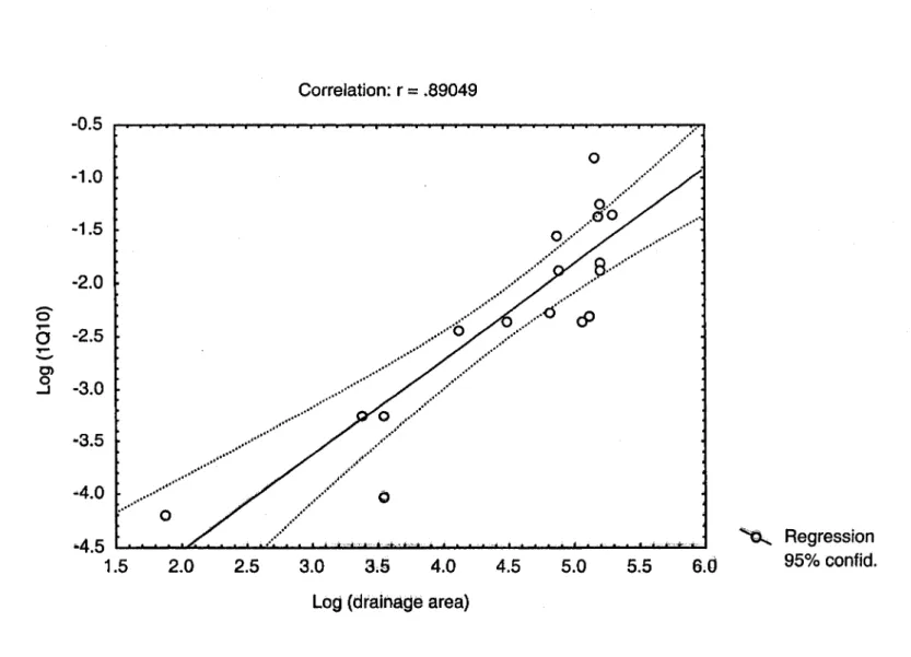
C) 0 -1 -0.5 -1.0 -1.5 -2.0 -2.5 -3.0 M3.5 -4.0 Correlation: r

=

.89049

o

•.•....•.. .'

..

'

.'

O'···

.efo .

?, ...

e ... .

...

..

...

."

...

..<5 ...

&

... .

... ··6

...

.'

... .

...

/

...

:

..

:,:~//./

....

..,

....

...

.

... .

•• + ~ •••••

...

.

...•.

o

...

o

...•.

"4.5 a...~""'"""' ____ .a...:;_~ ... ~..a...a.; ... ..o...&.. ... ...

1.5 2.0 2.5 3.0

3.5

4.0 4.5 5.0 5.5

6.0

Log (drainage area)

'0...

Figure

8. Regression between 10 year low flows with a one-day duration (lQI0) and drainage areas (from El

labi et al. 1994)

IV

(38)

-

0 (\J

0 _,...

--

0) 0 ...J

-0.5

-1.0

-1.5

-2.0

-2.5

-3.0

-3.5

-4.0

o

·4.5

...

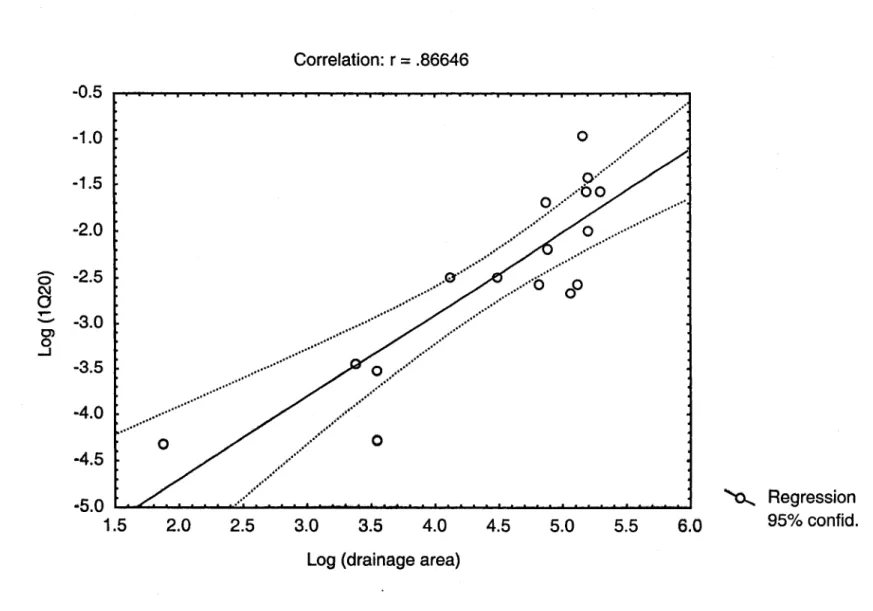
" Correlation: r

=

.86646 .'

....

" .' .' .'

....•..•..

o

..

'

..

'

o···

...

..

' .' .' .'

... 00

o .. ···

.. '

...

/

...

~

... .

0···

.·ô···

o //...

c9

...•...•.•.

.

'

.'

o

"

.5.0 ...

'-'-.a.-l.. ... ...:.'-I. ... ..&-..I ... .a.-I.. ... - ' - ' -... ..a....L ... _...,

1.5

2.0

2.5

3.0

3.5

4.0

4.5

5.0

5.5 6,0

Log (drainage area)

'0....

Figure

9. Regression between 20 year low flows with a one-day duration (lQ20) and drainage areas ({rom El labi et al.

(39)

-C\I

a

1"--

Cl 0 ...J 0.0 -0.5 -1.0 -1.5 -2.0 -2.5 -3.0 -3.5 " .' .' .'

....

Correlation: r

=

.89159 "

...•...

" "

....

.

' .' .' " " "

···0···

...

.'

o

...

o ... ····

0 ...

6 .

.. 0···

o ..

···ô···

O ···

..

'

0···

. 0 6 • •

-o

.'

-4,0

'--....O:;... _ _ ... _ _ ... _ ... _ ... _ _ _ ... _ _ _ ~ _ _ ... - ' -_ _ ... 1.5 2.0 2.5 3.0 3.5

4.0

4.5

5.0 5.5

Log (drainage area)

~ Regression

95% confid.

w

o

Figure 10. Regression between two year low flows with a seven-day duration (7Q2) and drainage areas (j'rom El Jabi

etai.

1994)

(40)

-

C\I 0

1"--

Cl

.9

Correlation: r

=

.91644

-0.5

o

_...•....

o ....

···i····

./ ... ·'::·· .. ' ... 9" .. "···"

..

... ,6···/··· ...

'····0 0 .... 0

...

.

•...

...

... ' .. 0···..--

/ .. ,

o

···

• ••••••• f f ' t • • • • • •

...

.

...

••• i'- 4'-... . ... 0

...

.

...•...

..

...

_....

,.,.

.

' .'

.•....

.

'

•...

...•.

.. 4.5

~

... """'"-' ... ...,,"""""-...

-.o....~ ... "--'-..-. _ _ ... ...

-1.0

-1.5

-2.0

-2.5

-3.0

-3.5

-4.0

1.5

2.0

2.5

3.0

3.5

4.0

4.5

5.0

5.5

Log

(drainage area)

~ Regression 95% confid.

Figure

11. 11.egression between 10 year low

fl,lJWS

with

a seven-day duration

(7Ql0)

and drainage areas (from El

(41)

-

0 C\I

0

f'..

-

0) 0 ..J Correlation: r = .89553 -0.5 -1.0 -1.5 -2.0 -2.5 -3.0

o

_...

.

'

o ...

'1/:) •...

o ... ····:·:::::::.:::;:::· .. · ..

··?···

... " .. ((... 0 -3.5 -4.0 -4.5

•..••..•...

.'

...

.'

.' .'

.'

.' .' .' .'

.'

-5.0 &....1.. ... - - . . . 0 - : . . ... _ ... - - - " " " - ' - _ ... .&...1..---&....1.. ... - - . . . ... ... 1.5 2.0 2.5 3.0 3.5 4.0 4.5 5.0 5.5

Log (drainage area)

~ Regression

95% confid.

Figure 12. Regression between 20 year low flows with a seven-day duration (7Q:10)

and

drainage

areas ({rom Ellabi et al.

1994)

(42)

160~---~

o

Regression 1 • Frequency analysis

120~---li

100 ..-. .!!!

...

E

--

CI) 80 C) a-ï III oC '; U

e

1/1 2i 60

i

40

l

jl

6

- f - - - ; n I - - - · - - - -.... .. -1 .• -f---iIf---"uiII;t, . - - - -.. -... 20 0 0

20

40 60 80 100 120

Return Period (years)

Figure

73. Comparison befween flood quantlles evaluafed by frequency analysls and by regression af

Development of a toolbox for assessment of aquatic habitat impacted by peat harvesting.