- FINAL REPORT -
Numerical Modeling of Gas Flow in the No. 1 Shaft
Waste Rock Dump, Sullivan Mine, B.C., Canada
Belkacem Lahmira and René Lefebvre
Low Atm osphe ric Tem pe rature High Atm osphe ric Tem pe rature
Institut national de la recherche scientifique Centre Eau Terre Environnement
Research Report R-970 July 2008
- FINAL REPORT -
Numerical Modeling of Gas Flow in the No. 1 Shaft
Waste Rock Dump, Sullivan Mine, B.C., Canada
Belkacem Lahmira and René Lefebvre
Institut national de la recherche scientifique, Centre Eau Terre Environnement
Research carried out under contract with Teck Cominco Limited
Report submitted to
Mr. Walter J. Kuit, Director, Environmental Science Teck Cominco Limited, Vancouver, Canada
Institut national de la recherche scientifique Centre Eau Terre Environnement
Research Report R-970 ISBN 978-2-89146-563-2
Executive Summary
The Sullivan Mine No. 1 Shaft Waste Rock Dump is located on a natural slope and covered by till. The outflow of oxygen-deprived gas through a leachate drainage pipe in an enclosure at the base of the dump resulted in four fatalities. Our mandate was to develop a numerical model to test the plausibility of physical mechanisms that were hypothesized to be controlling gas flow. The numerical model confirms that gas flow is controlled by atmospheric temperature. Gas comes out of the drainage pipe when atmospheric temperature is higher than an equilibrium value. On the other hand, air enters the pipe when atmospheric temperature is lower than the equilibrium value. The value at which there is no gas flow is equivalent to the average internal dump temperature. Steady state flow conditions are rapidly reached, in 15-20 minutes, even after the major simulated initial perturbation in atmospheric temperature and pressure. Since the system rapidly responds, pipe flow rates can closely follow atmospheric temperature changes. Gas flow is controlled by the relative buoyancy of the dump gas phase compared to atmospheric air, which is related to their relative densities. Barometric pressure has an insignificant effect on gas flow, as it barely modifies the relative densities of dump gas and atmospheric air. The presence of CO2 in the dump gas phase makes its molar mass equivalent to the one of
atmospheric air. This implies that dump gas composition does not either influence the relative densities of dump gas and atmospheric air. Changes in atmospheric air density are caused by atmospheric temperature variations, whereas the dump gas phase density is nearly fixed by the steady internal dump temperature. When atmospheric temperature is lower than the internal dump temperature, atmospheric air density is higher than dump gas density, inducing upward dump gas flow and air entry in the pipe. Instead, downward dump gas flow occurs and exits the pipe when high atmospheric temperature leads to an air density lower than dump gas density. Gas flow is facilitated by a coarse fill material that was placed in a ditch along the dump toe prior to covering of the pile. The coarse material focuses outward gas flow towards the pipe, and distributes inward gas flow from the pipe along the toe of the waste. Effective air permeabilities of waste rock and till cover significantly higher than initial estimates had to be used to exactly match observed pipe gas velocities. This could reflect the combined effects of coarse preferential flow paths in waste rock and localized variability in the cover. The relatively low permeability of the till cover still significantly limits gas exchanges between the dump and atmosphere. However, a very low permeability till cover is not required to get gas flow as observed at the site. On the contrary, a perfectly sealing dump cover would lead to a very different gas flow behavior. The model also shows that, under the conditions found in the No. 1 Shaft Dump, similar gas flow patterns would prevail without the pipe or without the till cover. The magnitude of gas flow would change though, gas flow being reduced without a pipe but enhanced without a cover. The No. 1 Shaft Dump is probably typical of some other covered dumps, which generally have steadily decreasing internal temperature and an oxygen-deprived gas phase, and where CO2 can
be generated if carbonates are present in the waste rock. Such conditions in other covered dumps could lead to gas flow behavior similar to what is observed at the No. 1 Shaft Dump. This gas flow behavior could potentially be found also in uncovered dumps having a mean internal temperature within the yearly range of variation of local atmospheric temperature.
Table of Content
1. INTRODUCTION 1
2. NUMERICAL MODEL DEVELOPMENT 3
2.1 MONITORING DATA REVIEW 3
2.2 SIMPLIFYING ASSUMPTIONS 6
2.3 MODEL DISCRETIZATION 8
2.4 MATERIALS AND CONDITIONS 9
3. NUMERICAL MODELING RESULTS 15
3.1 TEMPERATURE CONTROL ON GAS FLOW 16
3.1.1 HYDROSTATIC CONDITIONS 16
3.1.2 STEADY STATE GAS FLOW IN THE DUMP 16
3.1.3 STEADY STATE GAS FLOW IN THE PIPE 17
3.2 BAROMETRIC PRESSURE EFFECT ON STEADY STATE FLOW 18
3.3 TRANSIENT GAS FLOW CONDITIONS 19
3.4 GAS FLOW WITHOUT A TILL COVER 19
3.5 GAS FLOW WITHOUT A PIPE 20
4. DISCUSSION ON PROCESSES CONTROLLING GAS FLOW 23
4.1 PNEUMATIC POTENTIAL CONTROLLING GAS FLOW 23
4.2 GAS FLOW CONCEPTUAL MODEL 29
5. CONCLUSIONS 33
Tables, Figures and Appendix
(Tables, figures and appendix are found at the end of the report)
Tables
Table 1. Estimated gas densities in monitoring boreholes compared to atmospheric air densities
... 41
Table 2. Temperature and pressure conditions with corresponding pneumatic potential ... 42
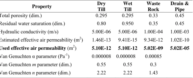
Table 3. Material properties ... 43
Table 4. Simulated gas velocities (m/d) in the waste rock dump ... 44
Table 5. Simulated gas densities and velocities through the pipe ... 45
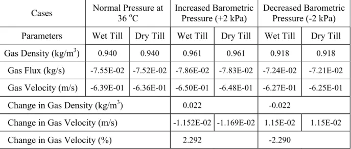
Table 6. Simulated pipe gas velocities related to changes in barometric pressure at 36 oC ... 45
Table 7. Steady state pipe gas flow velocities without a till cover ... 45
Table 8. Summary of monitored conditions in boreholes ... 46
Figures Figure 1. Location of Section 0+525 used to develop the numerical grid ... 49
Figure 2. Selected monthly temperature profiles in boreholes ... 50
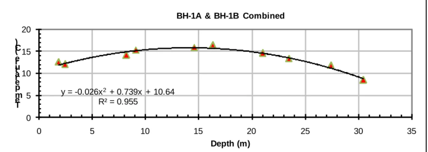
Figure 3. Second order polynomial fit to mean temperatures in boreholes BH-1A and BH-1B .. 51
Figure 4. Projection of boreholes on the numerical grid section ... 52
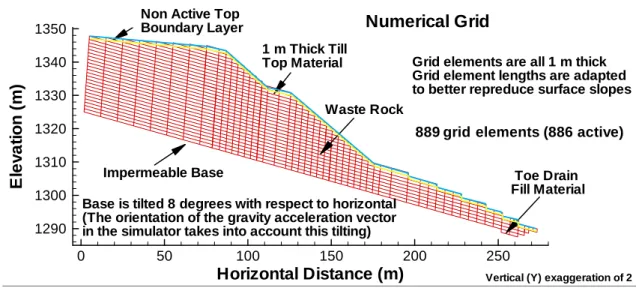
Figure 5. Boundary conditions and materials distribution in the numerical grid ... 52
Figure 6. Simulated conditions for low (top) and high (bottom) atmospheric temperature ... 53
Figure 7. Comparison of simulated and measured gas velocities in the pipe ... 54
Figure 8. Correlation between normalized temperatures and pipe gas velocities ... 54
Figure 9. Transient pipe gas velocities for various atmospheric temperatures (top) and pressures at 36 oC (bottom) ... 55
Figure 10. Transient gas mass in the dump for various atmospheric temperatures (top) and pressures at 36 oC (bottom) ... 56
Figure 11. Simulated conditions at 5 ºC without a till cover (bottom) compared to conditions with a dry till cover (top) ... 57
Figure 12. Simulated conditions without a pipe for a dry till cover at 5 ºC (top) and 36 ºC
(bottom)... 58
Figure 13. Pneumatic potential and streamtraces at 5 ºC for the dry till cover with the pipe (top), without a pipe (middle) and with a pipe but without a till cover (bottom) ... 59
Figure 14. Pneumatic potential and streamtraces at 36 ºC for the dry till cover with the pipe (top), without a pipe (middle) and with a pipe but without a till cover (bottom) ... 60
Figure 15. Vertical distribution of pneumatic potentials at 5 ºC (left) and 36 ºC (right) for the dry till cover with the pipe (top), without a pipe (middle) and without a till cover (bottom) ... 61
Figure 16. Comparison of the conceptual model of gas flow with numerical results for low (top) and high (bottom) atmospheric temperatures ... 62
Appendix
Appendix 1: Complementary simulation results and figures ...65 Appendix 2: Compilation of Gas Flux, Velocity and Mass ...77 Appendix 3: Estimation of material properties ...87
1. Introduction
This report documents the results of a research project carried out by INRS under a contract with Teck Cominco Limited titled “Development of a numerical model to provide a representation of physically-plausible mechanisms that could be controlling gas flow in the Sullivan Mine No. 1 Waste Dump”. A fatal accident occurred at the No. 1 Shaft Waste Dump of the Sullivan Mine, B.C. This accident is thought to be related to the downward flow of oxygen-deprived air originating from the waste dump. That air is presumed to have entered a water sampling enclosure located at the base of the waste dump through the water sampling pipe.
The objective of the project was to develop a numerical model to test the plausibility of various physical mechanisms that were hypothesized to be controlling gas flow in the Sullivan Mine No. 1 Shaft Waste Dump. The numerical simulator used was TOUGH AMD, which can represent physical processes related to AMD production in waste rock (Lefebvre, 1995; Lefebvre and Gélinas, 1995; Lefebvre et al., 1998, 2001b, 2001c, 2002; Smolensky et al., 1999; Wels et al., 2003; Sracek et al., 2004). Simulations used simplifying assumptions described in the next section, while keeping the model representative of conditions found at the site. A series of simulations were carried out to cover the range of material properties and conditions found at the site. Reports and data made available were reviewed and used to estimate material properties (Phillip and Hockley, 2007; Kimberley Incident Technical Panel, 2007). A review of available monitoring data was also made to develop a representative conceptual model of gas flow at the site that formed the basis for numerical modeling (personal communication of R. Lefebvre to D. Hockley, Dec. 2007). The validation and calibration of the model was achieved by the modeling of monitored conditions that were “reproduced” by the model. The key model parameters (air permeability of waste and cover) were adjusted to better represent the general gas flow behavior monitored at the exit pipe (and in a more general way within the dump).
The present scope of work is limited to the understanding of the No. 1 Shaft Waste Dump and does not include simulations that would aim to define the general conditions under which gas flow could represent a safety hazard at other waste rock dump sites.
2. Numerical Model Development
2.1 Monitoring Data Review
Figure 1 shows the location of monitoring boreholes and other monitoring facilities that were available when the numerical model was developed. The available data were reviewed to estimate material properties and develop a conceptual model of gas flow that was used as a basis for the numerical model development. The estimation of initial material properties is described in Section 2.4 and documented in Appendix C. This section briefly describes the temperature and gas composition data that were assessed in order to define representative model conditions. The conceptual model is described in Chapter 4, which discusses the processes controlling gas flow.
Figure 2 shows selected monthly temperature profiles measured in monitoring boreholes. Except for BH-1A and BH-1B, boreholes are shallow and temperatures are measured in the zone affected by cyclic yearly atmospheric temperature variations, which appears to be about 8 m deep in the waste rock dump. A sinusoidal fit to monitored atmospheric temperature showed that it could be represented by a mean surface temperature of 7.5 ºC and a total annual change in temperature of 31 ºC (not shown). For boreholes BH-1A and BH-1B, there are sufficient temperature measurements beyond the zone affected by cyclic surface temperature changes to determine a mean temperature profile using the available data (Figure 3). Average values of temperature were calculated at each measuring depth using the selected monthly profiles shown on the Figure 2. Data points obtained for both boreholes were combined in Figure 3 and a good regression could be made to the data with a second order polynomial.
Temperatures observed in the dump are very similar for BH-1A and BH-1B and clearly higher than the atmospheric mean value of 7.5 ºC. This implies that similar internal heat production occurs related to sulfide oxidation at these two locations. Furthermore, the relatively steady curvature of the temperature profile shown on Figure 3 could be indicative of heat production over the entire thickness of the pile. Similarly shaped temperature profiles observed at a Questa Mine, New Mexico, waste rock dump were shown to be related to lateral gas flow that could bring oxygen over the entire thickness of the dump (Lefebvre et al., 2002; Wels et al., 2003). However, the relatively low temperatures are indicative of moderate heat production that could
be related to limited gas flow and oxygen supply available to support sulfide oxidation. Caution must be used in the interpretation of temperature data as they may partly represent residual heat remaining to be dissipated following the placement of the till cover on the dump.
The observed thermal conditions in the No. 1 Shaft Dump show that temperatures are similar at central locations in the dump and remain quite stable throughout the year. This is an important observation as it was used to make the simplifying assumption that internal dump temperature could be fixed in the numerical model. These temperature profiles could also serve as baseline to be compared to long-term measurements of temperature in the dump. This comparison could provide a global indication of the effectiveness of the till cover. If the cover is effective, it should limit air inflow and oxygen supply, thus also limit heat production, such that temperature should be steadily decreasing in the dump. In the case of the No. 1 Shaft Dump, such interpretation will have to take into account the important gas exchanges occurring through the drain pipe. The pipe allows bypassing of the till cover at the base of the dump, which likely reduces the apparent performance of the cover in limiting gas exchanges between the dump and the atmosphere.
Another condition assessed on the basis of the monitoring data is the composition of dump gas. Gas composition was determined on dump gas flowing out of the drain pipe as well as in gas sampled from ports installed in monitoring boreholes. Equation 1, presented in Section 4.1, indicates that gas density is determined by its pressure, temperature and molar mass. The molar mass being itself fixed by the molar fractions and masses of the components present in the gas phase. In ARD-producing waste rock dumps, oxygen consumption would generally lead to a lower molar mass for the gas phase, as its own molar mass (32 g/mol) is higher than the mean dry atmospheric air molar mass (29 g/mol), which is controlled by the nitrogen molar mass (28 g/mol). This reduction of the waste rock dump gas molar mass is further accentuated by the increase in water vapor content (molar mass of 18 g/mol) if the internal dump temperature is high, which increases water vapor partial pressure and its proportion of the dump gas phase. In the No. 1 Shaft Dump, there is a relatively high proportion of CO2, which has a high molar mass
(44 g/mol). Dump gas outflow at the pipe can have more than 5 or 6% CO2, whereas
In waste rock dumps where temperatures are high, the reduction in density due to these temperatures is such that strong upward thermal gas convection occurs, as shown at Mine Doyon where values exceeding 60 ºC were observed (Lefebvre and Gélinas, 1995). The lightening of the gas phase caused by oxygen depletion can also lead to upward gas convection in dumps with lower internal temperatures, as demonstrated for the Nordhalde in Germany where internal dump temperatures were mostly lower than 16 ºC (Lefebvre et al., 1998; Smolensky et al., 1999). The moderate internal dump temperatures between 10 and 15 ºC observed in the No. 1 Shaft Dump and the high concentrations in CO2 in the dump gas could potentially lead to molar masses and
densities similar to atmospheric air. This could lead to reversals in the vertical flow tendency of dump gas relative to atmospheric air.
Table 1 shows results of calculations made to assess the effects of CO2 concentrations, internal
dump temperatures and atmospheric temperatures on the relative densities of dump gas and atmospheric air. Calculations were carried out for representative gas concentrations observed in boreholes. The presence of water vapor and relative humidity were considered. The first result of interest is the very similar humid gas molar mass for atmospheric air and dump gas for all boreholes. This implies that when atmospheric air has the same temperature as the dump, its density would be identical to dump gas density. Relative density is defined here as the ratio of borehole gas density over atmospheric air density. Buoyancy should make the dump gas tend to flow up when the relative density is lower than unity. Relative densities were calculated for a range of observed atmospheric temperatures (Low, Mean and High). On the basis of its relative density, Table 1 shows that dump gas should tend to flow upward when atmospheric temperature is low and downward when it is high. This is coherent with observed pipe gas flow directions as a function of atmospheric temperature. The relative density of dump gas and atmospheric air can thus be considered a potential driving mechanism for gas flow in the No. 1 Shaft Dump. These results further indicate that dump gas molar mass can be considered similar to atmospheric air, and this throughout the entire dump as all boreholes showed similar general gas flow tendencies. This supports the simplifying assumption that gas composition changes do not have to be considered in the numerical model. These results also indicate that dump gas composition, especially the presence of CO2, has to be taken into account while assessing potential dump gas
2.2 Simplifying Assumptions
The number of unknowns needed to specify the state of a numerical system depends on the number of phases and components considered (Pruess et al., 1999). Waste rock dumps in which acid mine drainage (AMD) is occurring are partially water saturated media within which oxygen consumption occurs due to sulfide oxidation (mostly pyrite), which leads to heat production (Lefebvre et al., 2001a). Numerical simulation of AMD in waste rock dumps thus involves the simultaneous estimation of four unknowns to determine the state of the system (gas pressure, water saturation, mass fraction of oxygen and temperature). The simulator also has to calculate the equation of state defining the equilibrium concentration of components (water, air and oxygen) in the two fluid phases (gas and liquid) as a function of temperature. This numerical problem is thus demanding, so that detailed numerical grids would require a long computation time to solve for the transient evolution of the system. For the numerical simulation of AMD production in waste rock, it is thus normally preferred to use relatively coarse grid elements, while capturing the most important features of the dump geometry and material distribution (Lefebvre et al., 2001b).
Compared to the general case of AMD in waste rock, specific conditions prevailing in the No. 1 Shaft Dump at the Sullivan Mine allow the modeled system to be simplified as follows:
• Thermal conditions. Isothermal (fixed temperature) conditions can be used with different temperatures assigned to the dump and atmosphere, but without considering heat transfer, thus avoiding the need to solve for temperature;
• Gas composition. Fixed gas composition, equivalent to atmospheric air, assigned to gas phases in the dump and atmosphere, thus avoiding the need to solve for gas composition; • Water flow. Fixed water saturations, at different values for waste rock and till cover,
imposed as residual water. This implies that no liquid water flow is represented, thus avoiding the solution of highly non-linear liquid flow under unsaturated conditions.
Isothermal conditions can be used since it was shown that the average temperature in the dump is relatively uniform and remains relatively constant throughout the year below a certain depth (Figures 2 and 3). Internal dump temperature is thus relatively independent of atmospheric
conditions. Different simulations were thus carried out with a fixed temperature assigned to waste rock but at different values of atmospheric temperature in contact with the dump surface. However, since the simulator cannot represent temperatures lower than 0 ºC, involving water freezing, mean dump temperature was shifted upward in numerical simulations as well as the atmospheric temperatures representing the range of variations observed at the site.
Fixed gas composition can be imposed in the numerical model because the dump gas phase was shown to have a mean molar mass similar to atmospheric air (Table 1). Although the dump gas phase is depleted in oxygen, which would lower the molar mass, it contains a proportion of CO2
that brings its molar mass close to atmospheric air (Table 1). Under such conditions, the dump gas phase composition will not significantly influence its density relative to atmospheric air. Using the same equivalent composition for both gas phases should thus lead to representative gas flow. This simplifying assumption avoids the need to represent oxygen consumption related to AMD production due to sulfide oxidation.
The dump is a partially water saturated media in which there is slow water infiltration, first through the till cover and then the underlying waste rock. However, the presence of the low permeability till cover spreads water flow relatively evenly throughout the year; even though it may vary seasonally, being expected to be higher during and following spring snow melt. Such conditions result in relatively stable water saturations whose influence on gas flow should remain quite constant throughout the year. Thus, including the solution of water flow in the system would not enhance the representation of gas flow. In order to impose water saturations representative of the system in the till cover and waste rock, while keeping water immobile, residual water saturation values were increased in the numerical model above imposed water saturations for each material. Under these conditions, the permeabilities of materials used as input in the numerical model correspond to effective air permeabilities controlling gas flow. Still, to take into account the effect of varying water saturations in the till cover, two simulation scenarios were used to represent “wet” and “dry” water saturation in the till cover and their corresponding effective permeabilities.
2.3 Model Discretization
Numerical modeling of gas flow related to AMD production in waste rock dumps is almost always carried out on two-dimensional vertical sections (Lefebvre et al., 2001b). Such models allow the representation of gas convection due to composition or temperature changes in the dump. Such convection has a strong vertical component, thus requiring the representation of vertical gas movements, but is most times not significantly changing laterally, thus not needing 3D models. Figure 1 shows the location of Section 0+525, which was used as a basis for the 2D vertical numerical grid of the No. 1 Shaft Waste Dump. This section was selected because it is representative of the central part of the dump and is surrounded by monitoring boreholes and the weather station. Since the dump has a wide central part, gas flow should predominantly be from the wide slope to the top surface and could thus be approximated as two-dimensional. A 2D vertical section numerical model having a similar width as the dump should thus be representative of the bulk gas flow in the dump.
Figure 4 shows the projected locations of boreholes on Section 0+525. Together, Figures 4 and 5 summarize the main features of the numerical grid and the distribution of materials. The grid represents the slopes at the surface of the dump as well as its base, which is inclined 8º relative to the horizontal. With TOUGH AMD, the numerical solution is independent of absolute coordinates and the geometry shown on Figure 5 was obtained by rotation and translation of the numerical grid for plotting purposes. All grid elements are vertically 1 m thick, but their lengths range from 2.5 to 10.0 m to allow a better representation of the different slopes. The horizontal transverse width of grid elements is 350 m in order to obtain a numerical model with a volume equivalent to the No. 1 Shaft Dump. The grid has a total of 889 elements, of which 53 are non active and serve to impose atmospheric conditions at the dump surface, and 1 element is non active to impose atmospheric conditions at the pipe located within toe drain fill material at the outside base of the dump. This pipe is where gas velocity, temperature and composition are monitored as gas flows in or out of the pipe. The area of the non active element representing the pipe in contact with an active drain element was assigned a value of 0.1257 m2, which represents the actual flow area of the pipe. This area should lead to representative simulated gas fluxes through the pipe.
2.4 Materials and Conditions
Figure 5 shows the distribution of materials and boundary conditions assigned to the numerical grid. At the surface of the dump, two single layers of 1 m thick elements are used to respectively represent non active (fixed) boundary conditions and the underlying till cover. Almost all the dump interior is assigned to waste rock material, except the high permeability fill material in the toe drain at the outer base of the dump. The pipe used to sample leachate and through which gas flows is within that drain material and it is a non active element to which atmospheric conditions are assigned. The inside limit and base of the dump are supposed impermeable and thus specified as no flux boundaries. Surface non active elements are assigned atmospheric temperature and pressure conditions. These non active elements are specified as having the same properties as waste rock in order not to artificially increase the thickness of low permeability till cover elements. Atmospheric temperature is uniformly assigned to non active boundary elements, including the dump surface and pipe. However, atmospheric pressure has to be applied with a value decreasing with elevation in accordance to the atmospheric air density in order to represent a stagnant hydrostatic gas column. Otherwise, the applied pressure could induce gas flow in the dump. Even though non active surface elements are assigned an atmospheric temperature different from the internal dump temperature, no heat transfer is considered. However, imposing atmospheric temperatures to non active surface elements provides inflowing air densities and viscosities representative of atmospheric temperature.
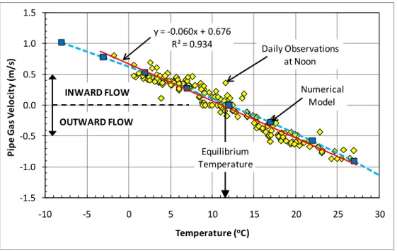
Monitoring data from the weather station show that temperature varies by about 30 oC, from -8 to 23 oC, and barometric pressure ranges from 85 000 to 88 000 Pa, with a mean of about 86 700 Pa (raw uncorrected pressures at the elevation of the weather station located on the dump). Monitoring data also show no gas flow through the pipe, so no gas exchange between the dump and atmosphere, when atmospheric temperature is around 10 to 12 oC. This “equilibrium” temperature thus represents the effective mean global gas temperature in the dump, considering that the dump gas phase has a molar mass equivalent to atmospheric air (Table 1). The magnitude of gas exchanges between the dump and atmosphere depends on the departure of atmospheric temperature from the equilibrium temperature. In order to simulate these gas exchanges, the numerical model thus has to represent the full range of 30 oC temperature
variations. However, the equation of state in TOUGH AMD cannot represent temperatures under 0 oC. Despite this limitation, since it is the departure in temperature relative to the equilibrium that controls gas exchanges, the model uses an equilibrium temperature of 25 oC, which allows the model to represent ± 15 oC changes without reaching negative values.
Table 2 summarizes the range of atmospheric temperatures and corresponding atmospheric pressures imposed as boundary conditions based on observed variations at the site. Base simulations at hydrostatic conditions, without gas flow in the dump, are carried out at 25 oC, the model temperature assigned to the dump. These simulations provide the initial conditions used for simulations carried out at other temperatures. The report highlights results obtained for the two “extreme” temperature cases at 5 and 36 oC representing the normal range of variation for atmospheric temperature at the site. Intermediate simulations were carried out every 5 oC between 5 and 45 oC to obtain a complete view of simulated conditions and verify if the gas flow behavior was “linear” between the two extreme values (results shown in Appendix 1). Table 2 also shows the atmospheric pressures corresponding to imposed atmospheric temperatures. These different atmospheric pressures strictly depend on the changes in temperature that induce different gas densities, thus leading to significant changes in barometric pressure due to the high elevation of the site. Table 2 shows pressure values imposed at the top of the dump and at the pipe located near its base. The barometric pressure imposed on the dump surface varies about linearly with elevation between these two values.
Table 3 summarizes the material properties derived from available data on the No. 1 Shaft Waste Rock Dump. Appendix C provides details on the estimation of these properties. Till properties were determined on the basis of available laboratory and field measurements. Using available grain size distributions, waste rock properties were estimated by comparison of its grains size distribution to analog waste rock whose properties were measured in the lab. Representative soil moistures of the till for wet and dry conditions were based on measured soil moisture profiles on the No. 1 Shaft Dump. A representative waste rock soil moisture was obtained by assuming capillary equilibrium with the till cover. Estimated capillary properties and relative permeability functions of till and waste rock are illustrated in Appendix C.
Material properties were modified from their initial estimate to calibrate and validate the model. The following criteria were used to determine if the model was representative and appropriately calibrated: 1) the direction (in or out) and magnitude of pipe gas flow as a function of atmospheric temperature; 2) the gas pressure gradients generated between the dump and atmosphere as compared to those measured at observation wells; 3) the gas flow patterns as compared to inferred patterns based on gas pressure gradients and gas composition measured in observation wells; and 4) the time for the system to reach steady state, as monitoring data show that pipe gas velocities and directions quickly follow changes in atmospheric temperature with a short lag time. Table 8 summarizes the main observations made by the No. 1 Shaft Dump monitoring system that form the basis of the model calibration criteria. These conditions and their inferred implications on gas flow are discussed in Section 4.2 on the conceptual model.
The effective air permeability is the property that had to be modified the most to calibrate the model. The value of effective air permeability had to be significantly increased, to at least 5x10
-12 m2 for the till cover and 5x10⁻⁹ m2 for waste rock, in order to reproduce the observed gas flow
behavior of the dump, especially the magnitude of pipe gas flow velocity. These values represent increases of more than 1 and 2 orders of magnitude, respectively, for the dry and wet till cover. For waste rock, the increase in effective air permeability over the initial estimate is 2 orders of magnitude. Such large increases above estimated values for the till cover, especially under wet conditions, were thought to indicate that the threshold effective air permeability required to calibrate the model is more likely related to local variability in the cover (fissures, grain size variations, compaction or thickness variations, etc.), than a poor initial estimate of the properties of “sound” till cover. The presence of such local variability is perhaps indicated by the observed localized melting of snow over the dump surface that could be due to preferential warm gas exit from the dump. Similarly, the large increase in effective air permeability for the waste rock over the initial estimate could reflect the heterogeneity of the dump and the presence of preferential gas flow paths through coarse high permeability material. The variability in the waste rock grain size appears to be confirmed by the recent geophysical and drilling investigations. Lahmira et al. (2007) have shown through numerical simulations that heterogeneous waste rock leads to water flow through fine-grained material, leaving coarse permeable material available for gas flow.
It is important to point out that simulations used “equivalent” homogeneous material properties to represent the till cover and waste rock that are likely heterogeneous. These equivalent properties departing from initially estimated properties do not imply that these initial estimates were necessarily wrong or that the cover is generally performing more poorly than what lab and field measurements would tend to show. Instead, these equivalent properties are through to be strongly influenced by the presence of preferential flow paths in waste rock and local variability of the till cover. Furthermore, properties of waste rock and till cover are not independent and other combinations of these properties could as well have led to model calibration. The presence of preferential gas flow paths through the waste could also have an effect on the equivalent cover permeability. The preferential flow paths would allow high pneumatic potential gas to be in contact with localized points of the cover. If some of those points were more permeable than the bulk of the cover, significant gas flow could result. When the model is calibrated by adjusting the equivalent homogeneous bulk properties of the waste rock and cover, these localized effects cannot be considered. The implication of this discussion is that the calibration of the till cover permeability should not be taken to represent a “correction” to the original estimates.
The most important evidence supporting the use of high equivalent air permeabilities for the till cover and waste rock is provided by the observed gas flow behavior of the dump itself. If the till cover were “perfectly” impermeable, the gas flow behavior would be quite different. Pressure equilibration between dump gas and the atmosphere would occur by gas circulation through the pipe. However, there would be zero gas flow under steady state after pressure equilibration. Since, on the contrary, it is gas buoyancy that is found to control gas flow, this process requires that “significant” gas flow takes place through the till cover, which supports the required increase in air permeabilities to calibrate the model. As will be discussed in Section 4, the observation that temperature controls pipe gas velocity is a clear indication that the mechanism of gas buoyancy is controlling gas flow in the No. 1 Shaft Dump.
Under the assumption that the effective air permeability required to calibrate the model did not reflect intact till cover but the potential effect of preferential paths through the cover, the same effective air permeability was used for both dry and wet till. If local variability controls the overall cover permeability, it would not be of interest to investigate values even higher than the
“threshold” required for calibrating the model. Under such conditions, this report presents no discussion of differences between dry and wet till simulations, as these lead to very similar results. The different porosity of wet and dry cover has an effect on gas velocity through the cover but not on gas mass fluxes.
3. Numerical Modeling Results
Gas flow can be generated by gradients in gas pressure, temperature or composition (Lefebvre, 2006). All these mechanisms can potentially contribute to gas flow in a waste rock dump. Heat production related to sulfide oxidation can increase temperature and lead to thermal gas convection (Lefebvre et al., 2001b). Barometric pressure changes can also generate pressure gradients between the gas present in a dump and the atmosphere and cause gas transfer with the atmosphere by compression or expansion of the dump gas column (Wels et al., 2003). Chemical reactions in dumps can consume oxygen related to sulfide oxidation and release CO2 by
carbonate dissolution, which can alter the molar mass and density of the dump gas phase, leading to gas flow related to positive or negative dump gas buoyancy relative to atmospheric air. Furthermore, these three gas flow processes are not independent as, for example, gas temperature or composition changes can alter gas pressure.
For the numerical simulation of gas flow in the No. 1 Shaft Waste Rock Dump, different emphasis was placed on the representation of the three potential gas flow processes. As explained before, gas flow related to gas composition changes was neglected a priori based on available data showing that dump gas molar mass is equivalent to the one of atmospheric air (Sections 2.1 and 2.2; Table 1). Special emphasis was placed on the representation of the effect of atmospheric temperature on dump gas flow, since pipe gas velocity monitored at the site was observed to be strongly correlated to atmospheric temperature. A systematic set of simulations were run every 5 ºC at temperatures below and above the equilibrium temperature fixed at 25 ºC for the purposes of numerical modeling. These simulations were made twice using the properties of dry and wet till cover. In this report, the emphasis is placed on the description of results for the minimum and maximum atmospheric temperatures of 5 and 36 ºC, respectively. Only the dry till cover case is discussed because, after the calibration process discussed in the preceding section, the dry and wet till cover cases produced very similar results. Complementary simulations were also carried out to investigate 1) the effect of high and low barometric pressures at 36 ºC for the dry till, 2) what would happen if there were no pipe, and 3) the impact of not having a till cover on the dump, in the last two cases at 5 and 36 ºC for dry and wet till.
3.1 Temperature Control on Gas Flow
3.1.1 Hydrostatic Conditions
Atmospheric pressure conditions are imposed on the numerical grid on the non active elements representing the surface of the dump and on the pipe, which is in contact with the atmosphere. The atmospheric gas column is itself static and at the simulation equilibrium temperature of 25 ºC, the dump gas column also has to be static. Simulated static conditions at 25 ºC are used as initial conditions for other simulations. Since gas flow is very sensitive to minute changes in pressure, it is necessary to carry out preliminary simulations at every temperature to be used later in order to define the hydrostatic pressure profile that will be used as boundary atmospheric conditions. These hydrostatic conditions are obtained by imposing pressure on a single non active element at the dump surface and then letting pressures equilibrate until there is no gas flow under steady state conditions. The pressures obtained for the boundary elements were then assigned to these elements that are made non active in subsequent simulations. Figures of these simulations are presented in Appendix 1 to show that insignificant gas flow was achieved and that boundary conditions used in the simulation doe not artificially induce gas flow.
3.1.2 Steady State Gas Flow in the Dump
The effect of variations in atmospheric temperature on gas flow in the dump was studied by applying temperatures ranging from 5 to 45 ºC and related barometric pressures on non active boundary elements at the surface of the dump and on the pipe. Dump temperature was maintained at 25 ºC and the initial dump gas pressures corresponded to hydrostatic conditions at 25 ºC. Due to such initial conditions, the onset of these simulations thus represents a sudden change in boundary temperatures and pressures, which induces transient dump gas flow conditions until the dump gas pressure distribution has equilibrated with imposed conditions. As these equilibrium conditions are reached, steady state dump gas flow related to imposed conditions is reached and pressure or gas flow patterns remain constant. These steady state flow conditions are the ones presented in this section. Figure 6 shows simulated gas flow for the base case conditions at 5 and 36 ºC with a dry till cover. Arrows represent gas velocity vectors whose dimensions are proportional to velocity and gas pressure is presented with a color scale.
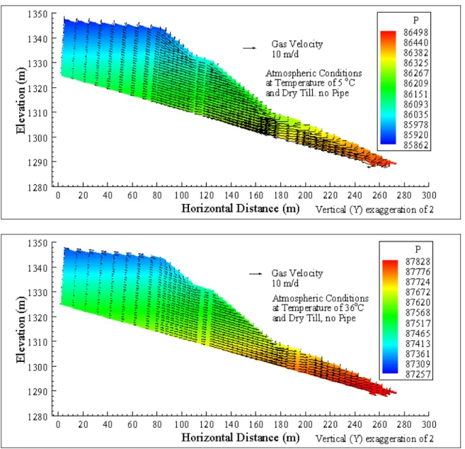
At the low atmospheric temperature of 5 ºC, gas flow is generally from the base to the top of the dump (upper graph, Figure 6). Most gas enters through the pipe and toe drain at the base of the dump and exits through the top surface of the dump. In the lower part of the dump there is some gas entering through the till cover over at the dump surface, whereas some gas exits through the upper part of the dump slope. Gas velocities are highest in the thin lower part of the dump and velocities are progressively reduced as gas enters in the thicker internal portions of the dump.
The lower graph of Figure 6 shows gas flow conditions at the high atmospheric temperature of 36 ºC. Under such conditions, gas flow is generally from the top to the base of the dump. There is limited gas exchange through the till cover over the dump slope, inward in the upper portion of the slope and outward in the lower part. As for the previous case, gas velocities are low in the thick upper portion of the dump and highest in its thin lower part. Gas flow patterns are overall similar, but in reverse direction, for the 5 and 36 ºC conditions, but the magnitude of gas flow is lower at 36 ºC than at 5 ºC.
The steady state dump gas flow conditions illustrated in Figure 6 are fixed for the atmospheric temperatures used. In the actual system of the No. 1 Shaft Dump, atmospheric conditions are continuously changing. So gas flow in the dump varies in magnitude and directions between the conditions illustrated at 5 and 36 ºC, which is a representative range of temperature change above and below the equilibrium temperature of 25 ºC used in simulations.
3.1.3 Steady State Gas Flow in the Pipe
Figure 7 compares measured pipe gas velocities as a function of atmospheric temperature to numerical simulation results. Pipe gas velocities provide the best indication of the importance and direction of gas flow in the dump. At the equilibrium temperature of 10-12 oC, there is no gas flow through the pipe, whereas pipe gas velocity is positive (into the pipe) at temperatures lower than the equilibrium and negative (out of the pipe) at temperatures above the equilibrium. Pipe gas velocity is strongly negatively correlated to atmospheric temperature (R2=0.934). Simulated pipe gas velocities very closely reproduce observations, showing that the model is properly calibrated. The model is also validated by comparison to other monitoring observations that are coherent with simulation results (next chapter). Table 5 compiles the pipe gas velocities
obtained at simulations carried out at various atmospheric temperatures and shows the 13 ºC lower actual site temperatures corresponding to the values used in simulations. Due to the use of the same effective air permeabilities of materials, simulations with dry or wet till cover have almost identical pipe gas velocities.
Observed velocities on Figure 7 tend to be higher (positively or negatively) than the regression line and simulated results. Perhaps this could be due to the fact that simulations represent steady state gas flow conditions, whereas the actual system is always dynamically adapting to varying atmospheric conditions, which involve higher velocities (next section). Figure 8 shows that there is a short time lag of 1 to 3 hours between reductions in temperature and increases in pipe gas velocities. The lag for decreasing velocities (increasing temperatures) is almost absent. Such a time lag would appear on Figure 7 as pipe gas velocities higher than the regression or steady state simulation results. However, some peak variations in atmospheric temperature are not followed by correspondingly as high measured pipe gas velocities, which would correspond to some of the observed velocities being lower than the regression or simulation prediction.
3.2 Barometric Pressure Effect on Steady State Flow
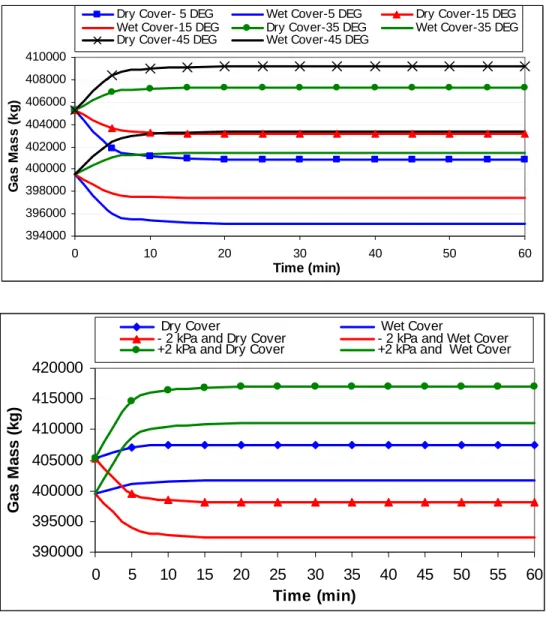
In order to evaluate the effect of barometric pressure changes on dump gas flow, simulations were carried out with increased and decreased barometric pressures (± 2 kPa) compared to the base case for the high atmospheric temperature of 36 oC, for dry and wet till covers. New hydrostatic pressure profiles were first simulated at the equilibrium temperature of 25 oC for these modified barometric pressures in order to impose appropriate boundary conditions. Compared to the base case, there is a very slight (2%) increase in steady state gas velocities at higher barometric pressure, whereas velocities are barely decreased at lower barometric pressure (Table 4b). Table 5 shows that changes in steady state pipe gas velocities are quite insignificant under different barometric conditions. Otherwise, dump gas flow patterns at different barometric pressures are almost identical to those obtained for the base case. For this reason, figures of simulated gas flow at changed barometric pressures were placed in Appendix 1. These results indicate that differences in barometric pressure have an insignificant effect on pipe gas velocity or the general direction or pattern of dump gas flow.
3.3 Transient Gas Flow Conditions
In order to investigate transient conditions in the dump following changes in temperature and barometric pressure, simulation printouts were generated every 5 minutes for a total time of 1 hour after the start of simulation. Figures 9 and 10 respectively show the evolution of pipe gas velocity and total gas mass in the dump after the initial “perturbation” corresponding to the start of a simulation. These figures show that after 15-20 minutes near steady state conditions are reached corresponding to the imposed atmospheric conditions. In the case of pipe gas velocities, the initial magnitudes at the onset of a simulation are very large and there can be reversals in flow direction at the start of a simulation compared to the direction reached at steady state. In the case of the total gas mass, the relative magnitude of the change is quite small, partially explaining why the transient period does not last long, along with the fact that gas exchanges through the pipe can rapidly transfer the gas mass required to reach the new steady state. These results demonstrate that the system can rapidly reach steady state conditions, even after the major perturbations imposed in numerical simulations. In the actual system, atmospheric conditions are progressively changing, rather than being subject of sudden variations. The short time required to reach steady state in simulations indicate that the system can dynamically adapt to progressive changes in atmospheric conditions. It would thus be uncommon to observe reversals in pipe flow direction due to changes in barometric pressure in the actual system, and any such changes would be short-lived.
3.4 Gas Flow without a Till Cover
In order to further investigate the role of the till cover on dump gas flow, simulations were carried out without a cover at 5 and 36 oC atmospheric temperatures. These simulations are meant to serve as basis for comparison to the base case. The material for till cover elements was replaced by waste rock, but these simulations otherwise use the same conditions applied to the base case, including the same mean internal dump temperature. This also includes the presence of the high permeability toe drain, even though this drain was in fact filled following cover placement. These simulations are not necessarily representative of the conditions that would actually prevail without a cover, but rather aim at better understanding the role of the cover under the conditions prevailing in the No. 1 Shaft Dump. These simulation results, especially gas
velocities, should thus only be interpreted relative to those obtained for the base case. If these simulations were carried out to represent actual conditions without a cover, it would then be important to consider more representative thermal conditions. Without a cover, the dump could have much more heat production due to the increase in oxygen supply, which would probably lead to higher mean temperatures.
Figure 11 compares gas flow patterns obtained with and without a cover at 5 oC under steady state. The scale of gas velocity vectors was changed compared to previous similar figures to better show gas flow patterns. The same scale is also used in both figures to facilitate comparison. Through most of the dump, velocities are higher without a till cover than with a cover, especially in the lower internal part of the dump. Gas entry or exit preferentially occurs at the base of the large dump slope. Table 7 shows that without a cover, pipe gas velocity is significantly higher than with a cover, at both 5 and 36 oC. Even though there is higher flow through the pipe, there is relatively less flow entering or leaving the dump through the pipe than elsewhere across the dump surface. These results have the important implication than even without a till cover, a dump in otherwise similar conditions as the No. 1 Shaft Dump would still have gas flow through a pipe at the base of the dump and would still be a personnel security threat when gas flow is downward, i.e. out of the pipe. Without a till cover, gas exchanges between the dump and atmosphere are unhindered, so transient conditions only last about 20 seconds, based on simulation printouts obtained every 10 seconds. Without a till cover, dump gas flow thus equilibrates almost instantaneously with changes in atmospheric conditions. These results show that even though the till cover allows enough gas flow to make buoyancy-driven gas convection possible in the dump, the presence of the cover still hinders gas exchanges between the dump and atmosphere.
3.5 Gas Flow without a Pipe
Again for comparison purpose, in order to further assess the importance of the pipe on gas exchanges, other numerical simulations were carried out without linking the pipe to the atmosphere at 5 and 36 oC atmospheric temperatures, with a dry and wet till cover. As the previous simulations without a cover, these simulations are meant to serve as basis for comparison to the base case. Besides the absence of link between the pipe and atmosphere, these
simulations use the same conditions applied to the base case, including the same mean internal dump temperature. Contrary to previous simulations without a cover, these simulations without a pipe could actually be representative of conditions that could prevail without a pipe. The time required to reach the present-day mean internal dump temperatures observed in the No. 1 Shaft Dump could be shorter without a pipe due to the likely lower air and oxygen supply to the dump.
Figure 12 shows simulation results at 5 and 36 oC for a dry till cover (compare to base case shown on Figure 6). Without a pipe, gas flows through the dump surface, rather than the pipe, in the lower part of the dump. This leads to lower velocities in the dump, especially in its lower part as shown in Table 4c. Despite lower velocities, gas flow patterns are otherwise similar as the ones obtained for the base case. These results show that even without the pipe similar gas flow circulation would occur under the conditions prevailing in the No. 1 Shaft Dump. However, these results also show that the pipe offers a preferential path facilitating gas exchanges between the dump and atmosphere. Without this preferential path, gas exchanges between the dump and atmosphere would be reduced and there would be less gas flow through the dump.
4. Discussion on Processes Controlling Gas Flow
4.1 Pneumatic Potential Controlling Gas Flow
Monitoring data and numerical modeling of the No. 1 Shaft Waste Rock Dump show that gas flow in that dump is controlled by atmospheric temperature. The physical process depending on temperature that is at the origin of gas flow is thermal convection due to dump gas buoyancy. Dump gas buoyancy depends on its density relative to atmospheric air. Gas (or air) density ρa
(kg/m3) is obtained from the following relations derived from the gas law (Lefebvre, 2006):
(
)
' ' i i a p x m M nm pm V V RT RT ρ = = = =∑
1Where M (kg) and V (m3) are respectively the mass and volume of gas. The mass of gas depends on its number of moles n (mol) and its molar mass m (kg/mol). The molar mass of a gas such as atmospheric air, which is a mixture of components i, is the sum of the products of molar fractions xi and molar masses mi of these components. The volume of gas is obtained from its
pressure p (Pa) and absolute temperature T’ (K) and the gas constant R (8.31 Pa⋅m3/mol⋅K).
In the case of the No. 1 Shaft Dump, it was already mentioned that the molar mass of dump gas is similar to the one of atmospheric air. Also, under steady state equilibrium, the mean gas pressure is fixed at a similar value by the prevalent barometric pressure both in the atmosphere and within the dump. The difference between dump gas and atmospheric air densities thus only depend on their respective temperature, gas density being inversely proportional to temperature.
The dump maintains a relatively steady mean internal temperature of about 10-12 ºC that it imparts to the gas phase present within the dump (Section 2.1, Figure 3). However, atmospheric temperature is quite variable, so that the density of the atmospheric air in contact with the dump will vary. Based on these principles and as shown by simulation results, in the case where atmospheric temperature is similar to the mean dump temperature, the density of atmospheric air will be the same as the one of dump gas and there will be no tendency for dump gas to flow. This is referred in this report as the “equilibrium temperature”. However, when atmospheric
temperature is lower than dump temperature, its density is higher than dump gas, which will tend to rise up through the atmosphere (positive buoyancy). On the contrary, when atmospheric temperature is higher than dump temperature, its density is lower than dump gas, which will tend to sink down through the atmosphere (negative buoyancy).
This process of buoyancy-driven gas flow controlled by atmospheric temperature departures from the dump “equilibrium temperature” is in qualitative agreement with the measured directions and magnitudes of pipe gas velocity versus atmospheric temperature. For this gas circulation process to occur, there has to be flow through the till cover and waste rock in the dump. The pipe directly connects the dump to the atmosphere, but flow also has to go through the dump top surface or through defects in the till cover. If the till cover were “perfectly” impermeable, the gas flow behavior would be quite different. Pressure equilibration between dump gas and the atmosphere would only occur by gas circulation through the pipe. However, there would be zero gas flow under steady state after pressure equilibration. Furthermore, flow through the pipe would be linked to barometric pressure changes, rather than atmospheric temperature variations. Thus, the strong relation of pipe gas velocity with atmospheric temperature and the insignificant effect of barometric pressure provide strong indirect indications that significant gas flow can occur through the dump surface.
The magnitude of dump gas flow through the dump is driven by the difference in pneumatic potential between the top and base of the dump that is caused by the buoyancy of dump gas relative to atmospheric air. The numerical simulator rigorously takes into account all processes contributing to gas flow as well as the compressibility of the gas phase. However, the simulator does not provide as an output the values of the pneumatic potential. These potentials much better show the processes controlling dump gas flow and gas exchanges between the dump and atmosphere than gas pressure. Thus, for the purpose of generating graphs, the following simplified form of the pneumatic potential Ψ (Pa) was calculated using numerical modeling
results (Lefebvre, 2006):
(
z z)
p g⋅ − + ⋅ = Ψ ρ 0 2Equation 2 is analog to the definition of hydraulic head, with a component of gas pressure p (Pa) and a component of elevation, which is the product of gas density ρ (kg/m3), gravitational acceleration g (9.81 m/s2) and elevation difference between the pressure measure point z (m) and an arbitrary reference elevation zo (m) (elevation is positive upward). This relationship is
neglecting gas compressibility, i.e. that density varies with pressure as shown by equation 1. However, over the short vertical interval of the No. 1 Shaft Dump, there is a very small change in density related to elevation and pressure. Pneumatic potentials were thus calculated “inside” the dump using the mean dump gas density corresponding to the mean internal dump temperature and pressure. The same relationship was also used for the surface boundary elements corresponding to atmospheric conditions. Pneumatic potentials for boundary atmospheric conditions indicate if atmospheric pneumatic potentials are in equilibrium with dump gas or would rather induce upward or downward dump gas flow.
Table 1 shows the pneumatic potential values calculated at the dump top surface and the pipe for the minimum, mean (equilibrium) and maximum atmospheric temperatures encountered at the site. The table also lists the mean dump gas and atmospheric air densities at these temperatures. The differences in density between dump gas and atmospheric air indicates that dump gas flow should generally be upward and downward, at respectively low and high atmospheric temperatures. The magnitude of that flow will depend on the pneumatic potential differences between the top of the dump and the pipe. The direction of dump gas flow is also shown by the fact that pneumatic potential is lower than at the pipe under low atmospheric temperature and higher at high temperature.
Respectively for simulations at atmospheric temperatures of 5 ºC and 36 ºC, Figures 13 and 14 show calculated pneumatic potentials corresponding to simulated conditions. Each figure shows conditions for three simulated cases: the base case with dry till cover and pipe, the case with dry till cover and no pipe, and the case without till cover but with pipe. The simulated high and low barometric pressure cases are not illustrated as these results are very similar to the base case, but with shifted absolute values of pneumatic potential. Figures 13 and 14 also show streamlines indicating gas flow paths within the dump. Arrows along these streamlines indicate the flow direction, whereas black squares are time markers whose spacing indicates 5 day flow duration.
White squares on the graphs indicate the four representative locations within the dump for which gas velocities are reported in Table 4.
The top graphs of Figures 13 and 14 represent simulated conditions for the base case, respectively at 5 and 36 ºC. Although dump gas flows in opposite directions at these different atmospheric temperatures, gas flow patterns have common features. First, most of the gas exchanges between the dump and atmosphere occur through the pipe (and toe drain) and the top surface of the dump. This is indicated by the fact that a vast majority of streamlines extends from the pipe to the top surface of dump. The area of the pipe and toe drain within the dump has a potential similar to the one of the dump surface boundary at atmospheric conditions. However, there is a large potential difference between the uppermost part of the dump and the boundary at the top dump surface (shown by the contrast in color representing potential magnitude). This indicates that a significant loss in potential occurs as gas flows across the till cover at the dump top surface. This feature is also apparent on the graphs of pneumatic potential versus elevation shown on Figure 15 that will be discussed later. There is limited exchanges through the till cover along dump slope as indicated a few streamlines originating from the slope. On that slope, gas is exchanged in different directions through the till in the upper and lower parts of the dump slope.
Table 4a shows that gas velocities are low in the interior and top portion of the dump, become higher in the center of the slope and are the fastest in the lower thin portion of the dump. This is also qualitatively indicated by the spacing of streamline time markers on Figures 13 and 14: farther apart markers indicate faster gas flow. Since little flow occurs through the till cover, there is about the same total gas flow rate from the top dump surface to the pipe located at the base of the dump. Gas velocity is thus related to the available gas flow cross section through the dump, which is much larger in the thick upper part of the dump than in the lower thin portion near the base of the dump. Gas velocities are higher for the case at low atmospheric temperature (5 ºC) than at high temperature (36 ºC) (Table 4a). This is due to the higher difference in pneumatic potential between the dump top surface and the pipe at 5 ºC compared to 36 ºC (Table 2). These differences in gas velocity between these two cases influence the total gas transit time through the dump. The transit time actually depends of the position within the dump. For the case at 5 ºC, if atmospheric temperature remained constant, it would take more than a month for gas to transit
through the lower part of the dump, whereas the transit time would be less than 20 days through the upper portion of the dump closer to the slope. In the case of the gas transiting across the dump slope, its transit time would be less than 10 to 15 days. Since gas flow is slower for the 36 ºC case, the total transit time would take more than 2 months in the lower part of the dump and in the order of 40 days in the upper portion of the dump close to the slope.
The middle graphs of Figures 13 and 14 show potentials and streamlines for the simulation case without a pipe, respectively at 5 and 36 ºC atmospheric temperatures. Compared to the base case, the absence of a pipe results in the same general flow direction and quite similar gas flow patterns through the dump. Without a pipe, the main difference compared to the base case is that gas has to flow through the till cover in the lower part of dump. There is an important potential loss as gas flows through the till (shown by the contrast in color related to potential magnitude). This is also apparent in Figure 13 that will be discussed later. Table 3c also indicates that gas velocity is decreased compared to the base case in lower part of dump. This is caused by more restricted gas exchanges between the dump and atmosphere in the absence of the pipe. As mentioned before, results for simulations without a pipe should only be compared to the base case as they are not meant to represent what would actually occur without a pipe, but rather what is the role of the pipe under the conditions presently prevailing in the dump.
The lower graphs of Figures 13 and 14 show potentials and streamlines for the simulation case without a till cover, respectively at atmospheric temperatures of 5 and 36 ºC. Compared to the base case, the absence of till cover leads to much faster gas flow in the dump. Since there is no till cover, in this case there is no potential loss across the dump surface. This leads to increased gas entry in the dump through the slope as well as the pipe. However, gas entry through the pipe is relatively less important, compared to gas entry through the slope. This is indicated by the fact that less streamlines are transiting through the pipe than what occurred for the base case. Table 3d shows that gas velocities are all higher through the dump than in the base case, except through the lower part of the dump. Again, results for simulations without a cover should only be compared to the base case as they are not meant to represent what would actually occur without a cover, but rather what is the role of the cover under the present conditions of the dump.
Figure 15 presents graphs of pneumatic potential versus elevation in the dump for simulated conditions prevailing after 12 hours, i.e. near steady state. Under these conditions there is equilibrium between imposed atmospheric temperature and pressure on the dump and gas flow within the dump. The three main simulation cases are presented: base case, no pipe, no cover. The high and low barometric pressure cases are not illustrated as they are very similar to the base case, but with shifted absolute values of potential. Table 2 showed that imposed atmospheric conditions lead to pneumatic potential gradients between the top surface of the dump and the pipe. On Figure 15, the potentials related to boundary atmospheric conditions appear as linear trends spanning the entire dump elevation range. For a given atmospheric temperature, these trends are the same for all three simulation cases since boundary conditions are identical for these cases. These linear vertical pneumatic potential gradients at the dump surface control the direction of dump gas flow. For low atmospheric temperature (5 ºC), the imposed boundary pneumatic potentials decrease with elevation, which leads to upward gas flow, whereas at high atmospheric temperature (36 ºC), the imposed potentials increase with elevation, which imposes downward gas flow.
The top graphs of Figure 15 correspond to the base case. Since there is a direct link between the dump and the atmosphere provided by the pipe and toe drain, the lower part of dump gas has the same pneumatic potential as the atmosphere. As gas flows through the dump, there is a pneumatic potential loss in the flow direction, upward for the 5 ºC case and downward for the 36 ºC case. This loss is more important (higher gradient) in the lower part of dump where the flow cross section is restricted, whereas very little potential loss occurs in the upper thick part of dump. The dump gas pneumatic potentials cross the atmospheric values at an elevation of about 1320 m. Above and below that elevation, the difference in potential between the atmosphere and dump gas leads to limited gas exchanges across the till cover due to its low effective air permeability. There is a large difference in potential between the atmosphere and dump gas at the top of the dump that corresponds to the potential loss occurring while gas flows through the till cover at the top surface of the dump.
The central graphs of Figure 15 show the trends in pneumatic potential with elevation for the cases without a pipe. The main difference relative to the base case is that the upper and lower
ends of the dump are at different pneumatic potentials than the atmosphere. Under these conditions, there are thus large potential losses as gas flows through the till cover at the base and upper portion of the dump slope, to either enter or exit the dump. The lower graphs of Figure 15 show conditions for the cases without a till cover. This time the main difference compared to the base case is that dump gas potentials are the same as atmospheric potentials along the entire slope of the dump. In the absence of cover, there is no potential loss as gas flows through the dump surface, which leads to overall larger dump gas potential gradient from the base to the top of the dump. This induces larger overall gas flows through the dump and more important gas exchanges between the dump and atmosphere without a till cover.
4.2 Gas Flow Conceptual Model
Table 8 summarizes the monitored conditions in observation boreholes, whose locations are shown on Figure 1 and projected positions on the numerical grid are indicated on Figure 4. The conditions compiled on Table 8 correspond to observations until the time the monitoring data were reviewed in December 2007. These conditions provide indications of gas flow conditions prevailing in the No. 1 Shaft Dump. On that basis, a gas flow conceptual model was developed, which guided the development of the numerical model used to simulate dump gas flow. That conceptual model is presented here so that the observations that formed the basis for its development can be compared to numerical simulation results. Such a comparison further validates the numerical model and ties together numerous observations made on conditions prevailing in the No. 1 Shaft Dump. Besides the conditions presented in Table 1, thermal conditions prevailing in the dump and gas densities estimated from boreholes gas compositions were also considered in the development of the conceptual model (Section 2.1).
Observed thermal conditions are the first data compiled in Table 8. Atmospheric temperature is presented as a reference and the values quoted for “Low”, “Mean” and “High” temperature are those obtained from a sinusoidal fit to the meteorological temperature data (Section 2.1). Values of borehole monitored parameters are representative of these different atmospheric temperature ranges. Temperature in boreholes listed in Table 8 is derived from measured monthly profiles that are affected by cyclic yearly air temperature variations as discussed in Section 2.1 (Figure 2). Boreholes BH-1A and BH-1B are the only ones deeper than the range affected by cyclic