Placement of Piezoelectric Laminate Actuator for Active
Structural Acoustic Control
M. Brasseur(1), P. De Boe(2), J.C. Golinval(1), P. Tamaz(3), P. Caule(4), J.-J. Embrechts(3), J. Nemerlin(4) (1) LTAS - Vibrations and Identification of Structures, Dept. ASMA,
(2) CAT – Wind tunnel,
(3) Sound and Image Techniques, Dept. EECS, (4) CAT-CEDIA, Dept. EECS,
University of Liège, B-4000 Liège, Belgium.
Abstract
The aim of this work is to investigate the problem of piezoelectric laminate placement. This problem is addressed in the case of modal identification and active control of plate like structures using piezoelectric laminates. The placement technique is based on the inspection of the controllability Grammian of the system expressed in a modal state-space coordinates. The controllability Grammian is able to quantify how structural modes are controllable with a set of predefined actuators. An initial finite element model or an experimental modal identification of the structure is required at the initial step. The procedure consists in making a selection of the smallest subset of actuators which gives a norm of the system transfer function as close as possible to the norm of the original full set.
As the study context consists in noise reduction in buildings, the second part of this paper describes an application of this technique on a wooden shutter box in order to reduce the acoustic transmission towards the inner room.
1 Introduction
This paper investigates the problem of placement procedure for distributed piezoelectric laminates. The success of piezoelectric materials mainly comes from their relative low-cost and light-weight properties and from the fact that piezoelectric laminates can be used as well in actuator as in sensor mode.
In many buildings, transmitted radiated noise (from air, road and railway traffics) is a persistent problem which is often poorly resolved by passive means, particularly at low frequencies. Sound radiation occurs as a result of the continuity of particle displacement at the interface between the structure and the surrounding medium. Acoustic insulation is then achieved by reducing the radiated sound. An alternative approach to the classical passive noise control is to use control inputs applied directly to the structure in order to reduce or change the vibration distribution with the objective of reducing the overall sound radiation. This technique has been termed Active Structural Acoustic Control (ASAC) [6]. ASAC techniques can then be used to control radiation of plane surfaces commonly encountered buildings.
An initial mathematical model (usually a finite element model) or an experimental modal identification of the structure is required at the initial step. Assuming that the stiffness and mass of the laminate actuators are negligible in comparison with the instrumented structure, the structural dynamics (in terms of resonance frequencies and mode-shapes) is independent of the number of candidates for actuator locations. The generated model is then used to compute the modal base of the structure which is truncated to retain the most representative set of structural modes.
The proposed placement technique is based on inspection of the controllability Grammian of the system using a modal state-space description. The controllability Grammian is able to quantify how structural modes are controllable with a set of predefined actuators. The procedure consists in making a selection of the smallest subset of actuators which gives a norm of the system transfer function as close as possible to
the norm of the original full set. The selection is performed independently of any control law. It is also assumed that the intervention of the control system doesn’t fundamentally modify the structure dynamics.
2 Piezo-structure
overview
2.1
Dynamics of piezo-structures
In the case of a structure instrumented with piezoelectric sensor/actuator, electromechanical relationships are added to the dynamics of the system to represent the contributions of the electrical degrees of freedom linked to the piezoelectric actuator and sensor (Saunders et al. [1]) :
q v C x v f x K x D x M s p s a a T = ⋅ + ⋅ Θ ⋅ Θ + = ⋅ + ⋅ + ⋅ && & ( 1 )
The first equation is commonly called the actuator equation and the second, the sensor one. The actuator equation exhibits the force generated by the piezoelectric actuator through the electromechanical coupling actuator matrix
Θ
a and the electrical potentialv
a applied between the electrodes of the element. When a piezoelectric actuator is supplied by a voltage amplifier, an added forceΘ
a⋅
v
a is applied on the structure.The sensor equation shows the relationship existing between the mechanical degrees of freedom x and the electrical charges
q
or potentialsv
s through the electromechanical coupling matrixΘ
sTand the capacitanceC
p of the sensor. When an external forcef
acts on the structure, the induced sensor signal depends on the electrical conditions applied at the electrode level :• Case 1 : open-circuit (
q
=
0
)(
)
0
1=
⋅
+
⋅
Θ
=
⋅
Θ
⋅
⋅
Θ
−
+
⋅
+
⋅
− s p s s p sv
C
x
f
x
C
K
x
D
x
M
T T&
&&
( 2 )The initial structure stiffness is modified by the corrective term sT
p s
⋅
C
⋅
Θ
Θ
−1 . However, this term isusually neglected when the partition of piezoelectric elements is small compared to the structure. Thus, the structural dynamics is not changed by the presence of the piezoelectric effect. The electrical voltage at the sensor electrode terminals is given by :
v
C
sTx
p s
=
−
−1⋅
Θ
⋅
. • Case 2 : short-circuit (v
s=
0
)q
x
f
x
K
x
D
x
M
T s⋅
=
Θ
=
⋅
+
⋅
+
⋅
&&
&
( 3 ) In this case, the capacitance of the sensor is eliminated from the output measurement by means of an appropriate analog circuitry (e.g. : a charge amplifier). Contrary to the previous configuration, the system dynamics is not affected by the electromechanical coupling.2.2
Sensor and actuator dynamic reduction
The dynamics of a piezoelectric system described by (1) is mechanically affected by the presence of the actuator/sensor transducers loading the structure (in terms of stiffness and inertia) : resonance frequencies and mode shapes are theoretically modified by the mechanical characteristics of actuator/sensor. If the transducer placement strategy would consist of a computation of a position index performance, it would induce that the eigen-value problem has to be solved at each iteration. This would be very costly and become prohibitive in case of large structures.
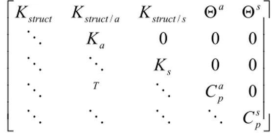
Therefore, when the partition of distributed transducers is negligible compared to the main structure, the idea is to neglect the inertia associated with the transducers as well as their stiffness (local stiffening neglected). In the proposed procedure, only the electromechanical coupling will be taken into account. As an example, let us consider a structure fitted with two decoupled piezo-laminates. Figure 1(a) shows the global stiffness connectivity of the initial system :
Θ
Θ
s p a p T s a s a s struct a struct structC
C
K
K
K
K
K
O
O
O
O
O
O
O
O
O
0
0
0
0
0
0
/ / ( 4 )where mechanical and electrical degrees of freedom (d.o.f.) are organized in such a way that :
{
}
T s a s a struct x x v q x x= ( 5 )where
x
structare the d.o.f.'s of the main structure andx
a,x
sare related to the actuator and sensor mechanical d.o.f.'s.When performing the finite element model (FEM) of the distributed transducers, a reduction of the transducer degrees of freedom (e.g. : using Guyans's reduction technique [2]) can then be performed as follows :
• Modeling of the distributed transducers.
• Reduction of the system to the structural interface degrees of freedom (see figure 1).
• Setting of the resulting transducer mass and stiffness matrix to zero (inertia and stiffening neglected). • Assembling of the modified transducer model with the main structure.
The d.o.f. vector of the resulting system is:
{
}
Ts a struct v q
x ( 6 )
When the partition of piezoelectric elements is small compared to the main structure, reduction errors on resonance frequencies and mode shapes are small, leading to an acceptable model for applying placement techniques. In the following, transducer models will be used in the condensed form.
(a) (b)
Figure 1 : Condensation of the piezo laminate at the interface degrees of freedom
3
The modal approach of controllability and observability
3.1
State-space modal representation
To apply the notion of controllability and observability, which is defined in the theory of control, it is convenient to express the structural representation of the system in the generalized form :
x
C
x
C
y
u
B
x
K
x
D
x
M
x x&
&
&&
&⋅
+
⋅
=
⋅
=
⋅
+
⋅
+
⋅
0 0 0 ( 7 ) wherey
is defined as the output vector and depends linearly of the structural displacements and velocities. The modal coordinates are defined by :m
x
x
=
Φ
( 8 )where the columns of
Φ
are the eigen modes of the conservative system. Let us define the state variables as the modal displacement and velocities : = m m m x x X & ( 9 )
The modal state-space representation of the system takes the form :
m m m
X
C
y
f
B
X
A
X
&
&
⋅
=
⋅
+
⋅
=
( 10 )with the following triplet :
[
mx mx]
m C C C B B Z I A = & = Ω − Ω − = , 0 , . . 2 0 2 ( 11 )where
Ω
=
diag
(
ω
1,
ω
2,
K
ω
n)
is the spectral matrix associated with the(
n
×
n
m)
modal matrix[
φ
1φ
2K
φ
nm]
=
Φ
. The modal mass, damping (assumed proportional) and stiffness matrix areobtained by the modal projection of
K
,D
,M
:1 1
.
.
.
2
1
,
.
.
.
.
,
.
.
− −Ω
=
Φ
Φ
=
Φ
Φ
=
Φ
Φ
=
m m T m T m T mD
M
Z
K
K
D
D
M
M
( 12 )In the same way, the modal input, displacement and velocity output matrices are defined as:
Φ
=
Φ
=
Φ
=
−.
.
.
.
0 0 0 1 x x m x mx T m mC
C
C
C
B
M
B
& & ( 13 )By simply rearranging the lines in the vector ( 9 ) in the following way :
{
x
x
x
x
}
T
m m mn n m m m1&
1K
&
( 14 )the modal state-space model takes the form of a block diagonal structure :
[
m]
m m mn m mn m mn mC
C
C
B
B
B
A
A
A
O
M
1L
1 1,
,
0
0
=
=
=
( 15 )The modal state-space representation has the dimension
(
2
⋅
n
m×
2
⋅
n
m)
which is much lower than the dimension of the structural model(
n×n)
since2
⋅
n
m<<
n
for a modal truncated system.3.2
Controllability and observability
In classical control theory, a linear time-invariant system of the form of equation (10) is fully controllable if and only if the controllability matrix :
[
B
AB
A
B
A
B
]
C
=
2 N 1−K
( 16 )has rank N=size
( )
A . In the same way, a linear time invariant system(
A, B,C)
is fully observable if and only if the matrix :
⋅
⋅
=
−1 NA
C
A
C
C
O
M
( 17 )has rank N. As clearly explained in Gawronski [6], these criteria, although simple, are not well adapted to practical applications :
• the level of controllability or observability is not quantified. These criteria give an answer in terms of yes or no.
• the computation of
c
oro
becomes prohibitive in the case of large systems.These two drawbacks may be alleviated by expressing the system properties in terms of Grammians. The controllability and observability Grammians are defined as follows :
( )
( )
t
e
C
C
e
dt
W
dt
e
B
B
e
t
W
t A t A t T o t A t At T c T T ⋅ ⋅ ⋅ ⋅∫
∫
⋅
⋅
⋅
=
⋅
⋅
⋅
=
0 0 ( 18 )The controllability Grammian reflects the ability of a perturbation u to influence the state of the system. The observality Grammian reflects the ability of a state
X
to affect the outputy
of a system. In the case of a time invariant system, the stationary solutions of ( 18 ) are given by the Lyapunov equations :0
0
=
⋅
+
⋅
+
⋅
=
⋅
+
⋅
+
⋅
C
C
A
W
W
A
B
B
A
W
W
A
T o o T T T c c ( 19 )The singular values of the Grammians product are invariant under linear transformation and are called the Hankel singular values :
(
W
cW
o)
i
N
i
i
=
λ
⋅
,
=
1
K
An important advantage of the modal state representation ( 9 ) is that the resulting controllability and observability Grammians are diagonally dominant (see Gawronski [3]) :
)
(
)
(
⋅
2×2≅
⋅
2×2≅
diag
w
I
W
diag
w
I
W
c ci o oi ( 21 )Diagonal entries of ( 21 ) and Hankel singular values can then be obtained as follows :
i i mi mi i i i mi oi i i mi ci
C
B
C
w
B
w
ω
ζ
γ
ω
ζ
ω
ζ
4
.
.
.
,
.
.
4
,
.
.
4
2 2 2 2 2 2≅
≅
≅
( 22 )which is a more efficient way to compute the Gammians than the resolution of equations ( 19 ).
3.3
Transfer function norm
The transfer function of a system, expressed in the state-space form, is given by :
( )
C
(
j
I
A
)
B
G
ω
=
⋅
⋅
ω
⋅
−
−1⋅
( 23 )
Transfer function norms
H
2,
H
∞,
H
Hankel may serve as a measure of the controlling ability of an actuator/sensor configuration applied to a system defined by(
A, B,C)
. In this paper, only the H2 norm, defined by :( ) ( )
(
)
(
) (
o)
T c T C W tr B B W C tr d G G tr G ⋅ ⋅ = ⋅ ⋅ = ⋅ ⋅ ⋅ =∫
+∞ ∞ −ω
ω
ω
π
* 2 2 1 ( 24 )will be considered. The second part of ( 24 ) shows the cross-connectivity between the output matrix C
and the observability Grammian
W
C (and vice-versa) on the system norm.For flexible systems in the modal state representation, H2 norm can be expressed in terms of the norms of modes. This modal decomposition gives then a visibility on each modal contribution. Taking the transfer function of the ith mode :
( )
mi(
mi)
mii C j I A B
G
ω
= ⋅ ⋅ω
⋅ − −1⋅( 25 )
the H2 norm of the ith mode can be estimated (see Gawronski [3]) by : i i i i mi mi i
C
B
G
γ
ω
ω
ζ
⋅
≅
⋅
⋅
∆
⋅
⋅
≅
2
2
2 2 2 (26)where
∆
ω
i=
2
⋅
ζ
i⋅
ω
i is the half-power frequency at the ith resonance. By using ( 24 ) and since the Grammians are diagonally dominant in the modal state-space representation, the H2 norm of the complete system is estimated by the rms sum of the modal norms :∑
==
mt n i iG
G
1 2 2 2 ( 27 ) where t mn
(<<
n
m) is the number of modes targeted for the control.3.4
Placement strategy for structural control
This technique addresses the problem of modal control. The aim is to select a minimal number of actuators that would control, as accurately as possible, the targeted modes. In the case of an actual structure, the procedure musttake into account geometrical constraints that may limit the number of candidate locations. Assuming that sensors are placed at all candidate locations (C is then fixed for comparison purpose only), the principle of the method is to compute, for each possible actuator location, the placement index
σ
ik. This index quantifies the excitation efficiency of the kth(
n
n
)
a
<
K
1
actuator on the ith(
)
t mn
K
1
mode byrelative comparison with the performance of the full set of actuators :
2 2 G G wik ik ik = ⋅
σ
( 28 )where
w
ik is a user-defined weighting coefficient that reflects the importance of the ith mode and the kthactuator in the application. A placement matrix can then be constructed by varying
B
0,C being fixed :actuator
k
mode
th 1 1 11⇑
⇐
=
Σ
th n n n ni
a t m t m aσ
σ
σ
σ
L
M
O
M
L
( 29 )Each terms of matrix
∑
show the ability of the kth actuator position to affect the ith mode. The globalactuator index, computed by the quadratic sum of the placement index for the kth actuator over all the
modes :
∑
==
nmt i ik k 1 2σ
σ
( 30 )reflects an averaged ability of the kth position to affect all the targeted modes.
In the case of a large (and complex) structure, the maximization of
σ
k alone is not a satisfactory criterion: too many locations have to be selected to guarantee a sufficient excitation of all the targeted modes. On the other way, a strategy based on the selection of the s1 higher placements for each mode will give too many locations with comparable efficiencies [3]. These locations can be extracted using an additional criterion based on the correlation of each actuator modal norm vector :
=
2 2 2 2 2 2 2 1 k n k k k t mG
G
G
g
M
( 31 )where Gik 2 is the H2 norm of the transfer function of the kth candidate actuator on the ith targeted mode. An assurance criterion (AC) is then used to distinct high correlated actuator candidate locations :
(
,)
1 0 2 2 ≤ ⋅ ⋅ = ≤ l k l T k l k g g g g g g AC ( 32 )When the assurance criterion
AC
(
g
k,
g
l)
is close to one, it means that these two actuator candidate locations excite the targeted modes with an equivalent efficiency. In this case, the actuator with the lower global index is removed.Based on the above analysis, the actuator placement strategy is established :
1) Construct the actuator placement matrix
∑
. In this way,n
acandidate actuator locations are selected.2) For each targeted mode, select the
s
m most efficient locations. The resulting number of actuators1
s for all the modes in consideration (i.e.,
t m m
n
s
s
1≤
⋅
) is then equal or much smaller than the number of candidate locationsn
a:a
n
s
1<<
3) Check the correlation between the s1 remaining actuator modal norm vectors
g
k. Keep all non-correlated locations withAC
(
g
k,
g
l)
<1
−
ε
, (0<ε
<1), and keep also the one with the higher indexσ
k for correlated actuators. The resulting number of actuator locations is nows
2<
s
1<<
n
a.4
Model identification strategy
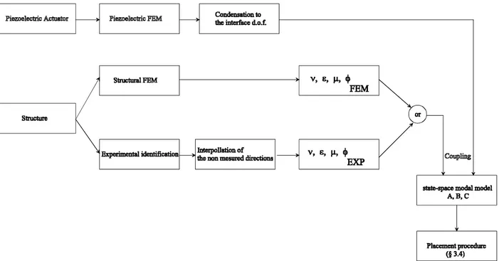
The placement strategy is based on the computation of the candidate actuator transfer functions. These transfer functions can be expressed in the state-space form. Therefore, the modeling of the actuator/structure coupling is required. The different preliminary steps of the placement strategy are shown in figure 2.
Figure 2: Fundamental steps for placement strategy
The piezoelectric element is modeled by finite elements. In our application, the model uses conventional 3-D isoparametric solid elements, improved by adding incompatible second order shape functions associated to nodeless degrees of freedom. This technique has been introduced by Bathe and Wilson [4]
and applied to piezoelectric structure by Tzou and Tseng [5]. The model is then condensed to the structural interface degrees of freedom as explained at section 2.2.
The structure can either be modeled by finite elements or by experimental modal identification. In the first case, modal parameters like modal mass
µ
, modal dampingε
, natural frequenciesν
and structural modesφ
are extracted. In the second case, the non-measured directions are interpolated at the measured nodes, before the extraction of modal parameters.The advantage of experimental identification is that characteristics of the real structure that are difficult to model (e.g. boundary conditions) are directly taken in consideration.
Thereafter the state-space model of the structure coupled with the piezoelectric element can be obtained. The
A
matrix depends of the modal parameters only. The actuator influence matrixB
is estimated by projecting the structural modesΦ
i (numerical or experimental) on the electromechanical coupling actuator matrices as a whole, i.e. :]
.[
.
1 1 a n a T m mM
aB
=
−Φ
Θ
Θ
L
where
Θ
ak is the electromechanical coupling of an actuator situated at the kth admissible location.Acoustical emission power is proportional to the velocity ([8],[9]) of the structure. Therefore in acoustic control applications, only the perpendicular velocity directions are important. Once the state-space model is estimated, the placement strategy can be applied as explained in 3.4.
5
Example of application
Two forms of active control of noise are generally available. The first one, termed ANC (Acoustic Noise Control [7] ), consists in generating with some secondary acoustic control sources, an acoustic field which destructively interfere in terms of radiated sound with the surrounding noise.
The second approach, called ASAC (Active Structural Acoustic Control), takes the direct relation between the structural vibrations and the emitted sound in consideration. Compared to the ANC approach, the
ASAC technique shows global attenuation performance of radiated sound with less control sources.
Instead of reducing directly the noise, ASAC uses control inputs applied directly to the structure in order to reduce or change the vibration distribution with the objective of reducing the overall sound radiation. To measure the level of noise radiated by the structure, microphones or structural vibration sensors can be used. Using piezoelectric laminates as structural sensors and actuators offers many advantages over other sensors and actuators as they are thin, lightweight and thus are easy to integrate in existing structures. Various modes of vibration present differing radiation efficiencies and some are better coupled to the radiation field than others. This suggests that in order to reduce sound radiation, only selected modes need to be controlled, rather than the whole response. In case of plate like structure, the first structural deformation mode is particularly emissive because no destructive interference appears between the air particles which are moving further to the structural displacements. On the other hand, structural modes composed by an equal number of nodes and anti-nodes behave like acoustic dipoles. The acoustic field tends to decrease significantly far from the vibrating structure.
5.1
Description of the problem
The objective pursued in the following example is to reduce the sound radiation emitted by shutter boxes (or containers) used in buildings (figure 3). The ASAC technique has to be applied to a wooden shutter box using piezoelectric actuators well positioned. Active control is limited to the frequency range of [0– 200 Hz]. Since passive isolation is effective beyond 200 Hz.
W a l l W i n d o w S h u t t e r " A c o u s t i c " W e a k p o i n t I n s i d e O u t s i d e
Figure 3: Description of the problem
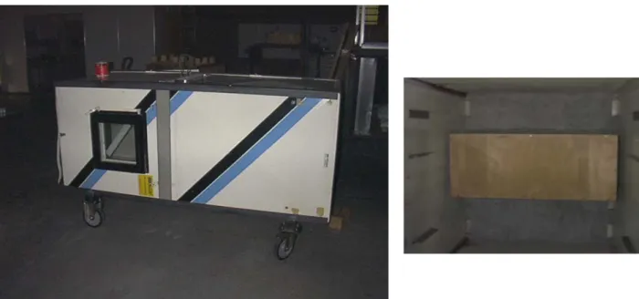
5.2 Prototype
testing
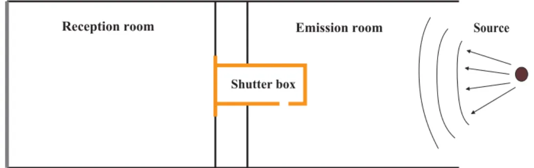
The control technique is first tested on the prototype shown in figure 4. This prototype placed in an anechoic chamber is installed in the CAT-CEDIA facilities (Acoustics Laboratory of the University of Liège) and consisting of :
- an emission room where an acoustic source is located, - the wooden shutter box to be tested,
- a reception room where noise reduction is measured.
S o u r c e E m i s s i o n r o o m
R e c e p t i o n r o o m
S h u t t e r b o x
Figure 5 gives a picture of the set-up in which the shutter box is integrated.
Figure 5: Used prototype placed in the anechoic chamber
Left: Whole set-up
Right: Inside view in the emission room
5.3
Modal analysis
In order to identify modal parameters of the wooden panel used for closing the shutter box, an experimental modal analysis has been performed. Results are presented in table 1.
Natural frequencies νi Type of mode Description of mode-shapes
96 [Hz] Odd (monopole) Complex mode
124 [Hz] Odd (monopole) Flexion
154 [Hz] Even (dipole) Torsion
229 [Hz] Even (dipole) Flexion
253 [Hz] Even (dipole) Complex mode
Table 1: Modal analysis results
At 96 Hz, it seems that the Helmholtz effect interacts with the structural vibrations of the panel. It should be noticed that the Helmholtz effect is easily avoided by an appropriate design of the shutter box slit. The origin of the mode at 253 Hz is not clearly identified. Nevertheless, it is probably due to a global coupling between the shutter box, the carrying structure and the acoustical cavity.
Figure 6 illustrates the three structural eigen modes identified in the frequency range of [ 0 – 260 ] Hz. In the working frequency range, only the mode at 124 Hz is odd and, thus, is particularly emissive. For this reason, only this mode has been targeted for noise reduction control.
0 0.1 0.2 0.3 0.4 0.5 0.6 0.7 0 0.05 0.1 0.15 0.2 0.25 0.3 0.35 −50 0 50 100 150 200 250 Mode at :124 Hz 0 0.1 0.2 0.3 0.4 0.5 0.6 0.7 0 0.05 0.1 0.15 0.2 0.25 0.3 0.35 −300 −200 −100 0 100 200 300 Mode at :154 Hz 0 0.1 0.2 0.3 0.4 0.5 0.6 0.7 0 0.1 0.2 0.3 0.4 −150 −100 −50 0 50 100 150 Mode at :229 Hz
Figure 6: Structural modes identified in the frequency range of [ 0 – 260 ] Hz
5.4
Optimal actuator placement
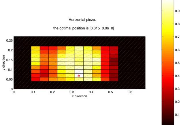
The placement procedure assumes that the piezoelectric laminate has fixed dimensions (compatible with commercial products). For practical reasons, the plate border is eliminated of the candidate positions. Vertical and horizontal orientations of piezoelectric laminates havebeen considered. Placement procedure described in § 3.4 is then applied and leads to an optimal horizontal position shown by a star in figure 7. This figure represents the placement index matrix
∑
(29).This optimal position is confirmed by physical considerations. To be efficient, the actuator has to be positioned in an area where the curvature (shown in figure 8) of the structure is maximum, inducing a maximum efficiency of the actuator. Indeed, an actuator placed on a zero curvature area would be unable to control the corresponding mode.
0.1 0.2 0.3 0.4 0.5 0.6 0.7 0.8 0.9 0 0.1 0.2 0.3 0.4 0.5 0.6 0 0.05 0.1 0.15 0.2 0.25 x direction y direction Horizontal piezo.
the optimal position is [0.315 0.06 0]
Figure 7: Placement index matrix and optimal horizontal position (*)
0 0.1 0.2 0.3 0.4 0.5 0.6 0 0.05 0.1 0.15 0.2 0.25 Curvature x direction y direction
Figure 8: Curvature of the structure
6 Conclusion
An actuator placement strategy based on the inspection of the controllability Grammian of the system expressed in a modal state-space coordinates has been presented. It allows to determine with low computation costs, the optimal number and positions of laminate actuators in order to control emissive vibration modes of the structure. An attenuation of sound radiation is then expected with the active control of these modes.
The proposed methodology has been successfully applied to a wooden shutter box. The selected actuator is best positioned to control the first structural mode (experimentally identified) which is the most emissive in terms of sound radiation. The active control implementation is now being tested. Encouraging results have already been obtained on a simplified prototype installed in the CEDIA laboratory of the University of Liège.
Acknowledgements
This work is supported by the ISACBAT project RW-ULG 114890 of the Walloon Region of Belgium, which is gratefully acknowledged.
References
[1] W.R. Saunders, D.G. Cole, H.H. Robertshaw, Experiments in piezostructure modal analysis for MIMO feedback control, Smart Mater. Struct, 3, 210-218, (1994).
[2] Maia, Silva, He, Lin, Skingle, To, Urgueira, Theoretical and experimental modal analysis, Research Studies Press LTD., Taunton, England (1997).
[3] W.K. Gawronski, Dynamics and control of structures : a modal approach Springer-Verlag, New-York (1998).
[4] K.J. Bathe, E.L. Wilson, Numerical methods in finite element analysis, Englewood Cliffs, NJ : Prentice Hall (1976).
[5] H.S. Tzou, C.I. Tseng, Distributed vibration control and identification of coupled elastic/piezoelectric systems : finite element formulation and applications, Mechanical Systems and Signal Processing, (1991) 5(3), pp. 215-231.
[6] C.R. Fuller, S.J. Elliott, P.A. Nelson, Active Control of Vibration, Academic Press Limited, London (1996).
[7] P.A. Nelson, S.J. Elliott, Active Control of Sound, Academic Press Limited, London, 1992.
[8] B.S. Cazzolato, C.H. Hansen, Active control of sound transmission using structural error sensing, Acoustical Society of America - Journal of Acoustic, 104(5), 2878-2889, 1998.
[9] W. Dehandschutter, K. Henrioulle, J. Swevers, Sas, State space feedback control of sound radiation using structural sensors and structural control inputs, Proceedings of Active 97, Budapest, 979-983, 1997.
![Figure 6: Structural modes identified in the frequency range of [ 0 – 260 ] Hz](https://thumb-eu.123doks.com/thumbv2/123doknet/6846426.191238/12.892.94.852.125.708/figure-structural-modes-identified-frequency-range-hz.webp)