Bond Indebtedness in a Recursive Dynamic CGE Model

(1)

Lemelin: Institut national de la recherche scientifique, Urbanisation, Culture et Société, 3465 rue Durocher, Montréal, QC H2X 2C6; Tél. (514) 499-4000; Fax: (514) 499-4065

andre.lemelin@ucs.inrs.ca

An earlier, incomplete version of this working paper was published in French in 2005 as CIRPÉE working paper 05-05, under the title « La dette obligataire dans un MÉGC dynamique séquentiel ».

Cahier de recherche/Working Paper 07-10

Bond Indebtedness in a Recursive Dynamic CGE Model

André Lemelin

(2)

(3)

Abstract :

In this paper, we present a minimalist version of a model of bond financing and debt, imbedded in a stepwise dynamic CGE model. The proposed specification takes into account the main characteristics of bond financing. Bonds compete on the securities market with shares, so that the yield demanded by the buyers of new bond issues increases as the cumulative bond debt grows relative to the stock of outstanding shares.

Restrictions are imposed on the maturity structure of bonds, so that it is possible to attain a reasonable compromise between a realistic representation of the evolution of the debt, and the demands on model memory of past variables values which impinge on the current period.

In the proposed model, the borrowing government reimburses bonds that have reached maturity, and pays interest on the outstanding debt. The prices of bonds issued at different periods and with different maturities are consistent with an arbitrage equilibrium. The supply of new bonds and of new shares is determined by the government’s and business’s borrowing needs. Security demand reflects the rational choices of portfolio managing households, following a version of the Decaluwé-Souissi model.

These notions are illustrated with fictitious data in model EXTER-Debt. The full specification of the model is described, and simulation results are presented which demonstrate model properties.

Key words : CGE models; recursive dynamics; bond debt; financial assets JEL codes : C68, D58, G1, H63

Résumé:

Dans ce texte, nous présentons une version minimaliste d'un modèle de la dette obligataire qui s'inscrit dans un modèle d'équilibre général calculable dynamique séquentiel. La spécification proposée tient compte des principales caractéristiques suivantes des obligations. Les obligations sont en concurrence avec une autre catégorie d'actifs, les actions, de sorte que le rendement exigé par les acheteurs de nouvelles obligations augmente à mesure qu'augmente la dette obligataire par rapport au stock d'actions en circulation. Des restrictions imposées à la structure de maturité des obligations permettent de définir un compromis raisonnable entre le réalisme de la représentation de l'évolution de la dette obligataire et le poids des valeurs passées des variables que le modèle doit conserver en mémoire.

Dans le modèle proposé, l'État emprunteur rembourse les obligations arrivées à échéance et paie les intérêts sur la dette en cours. Les prix des obligations émises à différents moments avec des échéances différentes sont cohérents avec un équilibre d'arbitrage. L'offre de nouvelles obligations et actions est déterminée par les besoins d'emprunt de l'État et des entreprises. La demande d'actifs reflète le comportement rationnel des ménages gestionnaires de portefeuille, conformément au modèle Decaluwé-Souissi.

Cette conception est illustrée au moyen de données fictives dans le modèle EXTER-Debt. La spécification complète du modèle est donnée et des résultats de simulations en montrent les propriétés.

Mots Clés: Modèles d'équilibre général concurrentiel; dynamique séquentielle; dette obligataire;

actifs financiers

(4)

(5)

INTRODUCTION

Bond indebtedness...

This article is about bond indebtedness in a recursive dynamic computable general equilibrium model. The objective of the proposed specification is to take into account the following characteristics of bonds :

• they are issued at a given date;

• they have a given nominal, or face value;

• they bear interest at a given rate relative to their face value;

• they have a maturity date, at which they are reimbursed by the issuer to the holder.

The policy interest of modeling bond indebtedness as accurately as possible is clear : any issuer of securities, including the government, runs the risk, beyond a certain level of indebtedness, that his/her credit rating fall, which then forces new issues to bear interest at increased rates, and may even close the door to further borrowing.

in a recursive dynamic CGE model

A recursive dynamic model is different from an intertemporal model in that, in the latter, the optimizing behavior of economic agents encompasses all periods up to the time horizon simultaneously, while in recursive dynamics, the system’s state in each period depends only on past and current values of variables, not on future values (though it may depend on expected future values).

In principle, the model’s « memory » at any given time could reach back to every preceding period, beginning with the initial situation. But if a simulation extends over more than very few periods, the number of variables quickly becomes quite large. That is why, practically speaking, modeling strategies try to condense memory of the past into a small number of stock variables. For instance, the stock of capital at the beginning of a period typically summarizes all of the previous history of investment and depreciation (except in vintage models, where the number of generations is nonetheless usually kept low).

With regard to debt in the form of bonds, there are three aspects which call into play the model’s « memory ». First, the amount of interest payable depends on the face values and the interest rates of all past issues which have not yet been redeemed. Second, the amount of debt that

(10)

comes to maturity (and must be redeemed or refinanced) depends on the face values and maturity dates of all past issues still outstanding. Finally, the level of indebtedness is the result of past issues, that is, in the case of government, of the cumulative deficit of past government expenditures and investment spending.

In this essay, we propose a model which can account for interest payments, debt redemption at maturity, and the level of indebtedness, while maintaining acceptable model memory requirements.

Our model does not pretend to be immediately operationnal. Our objective is rather to present the general principle of the proposed specification in a minimalist form. It is a model without money, where only relative prices matter. Although it has asset markets, it cannot be considered to be a financial model. Moreover, there is no financial intermediation in the model.

A minimalist framework

Even a minimalist framework requires that there be an asset competing with bonds. Indeed, in order to represent the rise in the cost of borrowing and the erosion of borrowing capacity which results from higher indebtedness, the rate of interest on new issues must depend on the stock of debt. In a micro-founded approach, that requires competition to government bonds from of at least one other asset. When government bonds compete with another asset, the greater the stock of outstanding debt, the lower the market valuation of bonds, and the higher the interest rate on new government bond issues.

That modeling strategy also implies that the demand for assets reflect the portfolio allocation behavior of asset holders. Moreover, not only current savings, but all of the wealth portfolio must be reallocated in every period. Because, if only current savings are allocated among currently offered new assets, equilibrium prices of new issues are independent of outstanding stocks1_. These notions are illustrated in the EXTER-Debt model, which was developed to demonstrate the feasibility of the modeling principle presented in this paper. It was constructed on the basis of the EXTER_DS2_{model, which itself derives from the EXTER}3_model.

1 The latter approach is Robinson’s (1991) or Decaluwé, Martin and Souissi’s (1992) « flow of funds » approach. 2 Forthcoming.

3 Decaluwe, Martens, Savard, 2001. Details of the EXTER model are available on the Poverty and Economic Policy (PEP) website (http://www.pep-net.org/) : see the « Core Training Manuals on CGE Modeling » section in the MPIA training material, Volume 2 – Basic CGE models (training material).

(11)

In EXTER-Debt, we make several assumptions to make the model as simple as possible, even at some cost in terms of realism, so as not to distract from the illustration of the proposed modeling approach.

Our model has four agents : households, businesses, government, and the Rest-of-the-World (RoW) :

• Government issues bonds to finance its current deficit and public investment. • Businesses issue shares to finance their investment expenditures.

• Households own a portfolio of both assets.

• The RoW owns only shares (one of our many simplifying assumptions).

Time structure of EXTER-Debt

We shall see below that financial asset markets are to be represented as transactions on stocks of assets. So it is of utmost importance to clearly specify the meaning of the time subscripts attached to stock variables. It is a matter of convention, of course, but it is preferable that the convention be explicit.

In this model, agents (households, businesses, government) make their decisions at the beginning of each period in the form of strategies (such as demand or supply functions), according to equilibrium values which they take as given (as is the case with prices in perfect competition). The equilibrium conditions determine end-of-period values.

Securities issued during a given period t start paying income (interest or dividends) in the following t + 1 period. Securities redeemed during a given t period bear interest in that same final period. But securities redeemed in period t are excluded from the stock of outstanding securities offered to portfolio owners during period t.

Organization of the paper

The following section defines bond price calculations, and develops the calculation formulas for the amount of bonds to be redeemed in the current period, interest to be paid on outstanding bonds, and the aggregate market value of bonds issued in previous periods not currently coming to maturity. The next section describes the Decaluwé-Souissi portfolio allocation model applied to households. Section 3 details asset market equilibrium conditions. In section 4, after a presentation of the Jung-Thorbecke investment demand function, closely related to Tobin’s « q » theory, the key role of the user-cost of capital and its relationship to the asset market are

(12)

examined. Simulation experiments, conducted on the basis of artificial data, are analyzed in the following section. The paper ends with a summary and conclusions.

1. BOND MARKET

1.1 The price of bonds

Recall that securities issued during a given period start paying income (interest or dividends) in the following period. Securities redeemed during a given period bear interest in that final period. But redeemed securities are excluded from the stock of outstanding securities offered to portfolio owners during that period.

A bond issued at face value in period t, maturing in period t+1, and bearing interest at current rate i_tB, has a cost of acquisition in period t of 1, and a capitalized value in t+1 of (1+i_tB). After

the payment of interest due in period t, a bond issued in period t–θ, coming to maturity in period

t+1, and bearing interest at rate i_tB₋_θ, has a capitalized value in t+1 of (1+ B

t

i₋_θ ). Assuming there

is no risk aversion, in equilibrium, a portfolio manager must be indifferent between these two securities. Their relative price in period t is therefore

B t B t i i + + ₋ 1 1 _θ

Next, a bond issued in period t at face value, coming to maturity in period t+τ, and bearing interest at current rate i_tB, has a cost of acquisition in t of 1, and a capitalized value in t+τ of

(1+i_tB)τ. After the payment of interest due in period t, a bond issued in period t–θ, coming to

maturity in period t+τ, and bearing interest at rate B t

i₋_θ , has a capitalized value in t+τ of

(1+ B t

i₋_θ )τ. In equilibrium, a portfolio manager must be indifferent between these two securities.

Their relative price in period t is therefore

(

)

( )

τ τ θ B t B t i i + + ₋ 1 1

Let us now compare two bonds issued in period t at face value, and bearing interest at the current rate i_tB, one coming to maturity in t+1, and the other in t+τ . Their relative price depends

(13)

on expectations relative to interest rates which will prevail in t+1 and in every period until t+τ −1. Under myopic expectations, the relative price of these two bonds will be 1, because the capitalized value is the same in both cases : the capitalized value of the bond coming to maturity in t+1 will be reinvested from period to period at the expected constant rate of i_tB, until t+τ .

So, in general, under myopic expectations relative to interest rates, the price of all bonds issued in the current period is the same. But the relative price of outstanding bonds (other than those issued in the current period) depends on the rate of interest of each one of them (and, therefore, on the period of issue) and on the number of periods remaining to maturity. The price at time t of a bond issued in t−θ, coming to maturity in period t+τ, and bearing interest at rate B

t i₋_θ , is given by

(

)

(

)

(

)

τ τ θ τ θ θ B t B t t i i PO + + = + − 1 1 , [001]

As expected, the price of bonds issued in period t (θ = 0) is equal to 1. And the price of bonds maturing in period t (τ = 0), which will be redeemed at face value, is also equal to 1.

In what follows, the price of bonds issued in t–1, and coming to maturity in t+1

( )

(

₍

₎

)

B t B t t i i PO + + = − 1 1 2 , 1 1 [002]

plays an important part. Indeed, we shall take advantage of the relation

(

1 ₁

) (

1 B

)

_t

( )

1,2 t B t i PO i = + + ₋ [003]

which, by recursion, leads to

(

1+ ₋_θ

) (

= 1+ ₋_θ₊₁

)

₋_θ₊₁

( )

1,2 =

(

1+ ₋_θ₊₂

)

₋_θ₊₂

( )

1,2 ₋_θ₊₁

( )

1,2 =_L t t B t t B t B t i PO i PO PO i [004]

(

) (

)

_∏

( )

= − + − = + + _θ θ _θ 1 2 , 1 1 1 s t s B t B t i PO i [005]

To streamline notation, we define

( )

(

₍

₎

)

B t B t t B t i i PO P + + = = − 1 1 2 , 1 1 [006]

(14)

so that [005] is now written as

(

) ( )

∏

= − + − = + + _θ θ _θ 1 1 1 s B s t B t B t i P i [007]

We also have the following equivalence

(

)

(

)

( )

τ θ θ τ τ θ τ θ θ _⎟⎟ ⎠ ⎞ ⎜ ⎜ ⎝ ⎛ = + + = +

∏

= − + − 1 1 1 , s B s t B t B t t P i i PO [008]

1.2 Redemption of bonds at maturity

In the basic model, it is assumed that the maturity structure of issues in all periods is the same. But it is not assumed that the maturity structure is flat, i.e. that an equal fraction of the bonds issued in a given period come to maturity in each following period until there are none left. Rather, that fraction is defined separately for every term m ≤ M, M being the longest maturity admitted in the model.

So it is assumed that a constant fraction f_m of the bonds issued in each period t is for a term of

m ≤ M periods. Of course, consistency requires

1 1 =

∑

= M m m f [009] Let τ t B

Δ be the stock of bonds issued in period t and coming to maturity in period t+τ, and ΔB_t, the number of new bonds of any term issued in period t. It follows that

t m m t f B B = Δ Δ , for m ≤ M [010] and, of course, t M m m t B B =Δ Δ

∑

=1 [011] With the term structure so specified, one can compute the amount to be paid in redemption in period t as

∑

= − = − Δ = Δ = M m m t m M t t B f B REMB 1 1 θ θ θ [012]

It is admittedly somewhat restrictive to impose the assumption of a constant maximum term and maturity structure of issues. But that kind of restriction is unavoidable given the form of price

(15)

equations [001] or [008] : for lack of a maximum term, the equations, developed below, of the amount of interest to be paid and of the value of outstanding bonds, would involve theoretically infinite summations. We have been unsuccessful in our efforts to reduce these infinite summations to closed analytic forms (such as can be done for a converging geometrical series). Because recursive dynamic models do not accommodate calculations that involve variables from an indefinitely long past, some form of simplifying hypothesis had to be made, and we think the assumption which is made here is a reasonable compromise.

Note that, although the redemption of bonds having reached maturity is a negative cash flow, it is not part of current government expenditure and does not affect the level of savings. Even if agents’ asset-liability balance is not explicit in the model, it is obvious that the redemption of bonds at maturity is a simultaneous decrease of government assets and liabilities, together with a change of nature for one element of the households’ portfolio.

1.3 Interest currently payable on bonds

According to the time structure laid out earlier, the total amount of interest which a debtor must pay in a given period is the sum of interests payable on the remainder of bonds issued in all previous periods and not yet redeemed (which includes bonds coming to maturity in the current period, but excludes those issued in the current period).

It is demonstrated in Appendix 1 that the amount of interest due on outstanding bonds is given by

( )

∑

∏

∑

= − − = − − = − = − = − − = − ⎥ ⎥ ⎦ ⎤ ⎢ ⎢ ⎣ ⎡ Δ ⎟ ⎟ ⎠ ⎞ ⎜ ⎜ ⎝ ⎛ − − Δ ⎟ ⎟ ⎠ ⎞ ⎜ ⎜ ⎝ ⎛ − ⎟ ⎟ ⎠ ⎞ ⎜ ⎜ ⎝ ⎛ + = Δ ⎟ ⎟ ⎠ ⎞ ⎜ ⎜ ⎝ ⎛ − = M t m m t m m s B s t B t M t m m B t t B f B f P i B f i INT 1 1 0 1 0 1 0 1 1 0 1 1 1 1 θ θ θ θ θ θ θ θ θ θ [013]

where, by convention, f₀ = 0. Let us define outstanding face-value debt at the beginning of period t (before debt coming to maturity in period t is redeemed, and before new bonds are issued) as DN_t:

∑

= − − = Δ ⎟ ⎟ ⎠ ⎞ ⎜ ⎜ ⎝ ⎛ − = M _t m m t f B DN 1 1 0 1 θ θ θ [014]

(16)

( )

_t M t m m s B s t B t M t m m B t t i f B i P f B DN INT − ⎥ ⎥ ⎦ ⎤ ⎢ ⎢ ⎣ ⎡ Δ ⎟ ⎟ ⎠ ⎞ ⎜ ⎜ ⎝ ⎛ − ⎟ ⎟ ⎠ ⎞ ⎜ ⎜ ⎝ ⎛ + = Δ ⎟ ⎟ ⎠ ⎞ ⎜ ⎜ ⎝ ⎛ − =

∑

∏

∑

= − − = − = − = − − = − 1 1 0 1 0 1 1 0 1 1 1 θ θ θ θ θ θ θ θ [015]

In accordance with national accounting principles, interests paid on public debt are a transfer, which is added here to other public transfers. Transfers made as interest payments on public debt are distributed among households in fixed shares (a simplifying assumption) :

t PIN h t h t h TG INT TGINT _, = _, +λ [016]

where TG_h,t is the exogenous amount of public transfers to household h, and INT_t is the amount of interests paid on the public debt.

Contrary to the redemption of bonds having come to maturity, the payment of interests is part of current expenditures and affects government savings.

1.4 Aggregate value of outstanding bonds

The aggregate value of outstanding bonds issued in past periods is not the same thing as face-value debt. The latter is the sum of the face face-values of bonds issued in the past and not yet redeemed. The aggregate value of outstanding bonds, on the other hand, is measured without reference to the face value of bonds issued in the past : rather, it is the current market value of all outstanding bonds, except those issued in the current period, after redemption of those which have come to maturity.

Once bonds coming to maturity have been redeemed, the market value of bonds issued in the past and still outstanding in period t is given by

(

)

∑ ∑

− = − = + − Δ + = 1 1 1 , M M t t t PO B B θ θ τ τ θ θ τ θ θ [017]

where the price at time t of a bond issued in t−θ, coming to maturity in t+τ, and bearing interest at rate B

t

i₋_θ has already been shown to be

(

)

(

)

( )

τ θ θ τ τ θ τ θ θ _⎟⎟ ⎠ ⎞ ⎜ ⎜ ⎝ ⎛ = + + = +

∏

= − + − 1 1 1 , s B s t B t B t t P i i PO [008] and where t m m t f B B = Δ Δ , for m ≤ M [010]

(17)

Therefore,

∑ ∑ ∏

− = − = = − + + − Δ ⎟ ⎟ ⎠ ⎞ ⎜ ⎜ ⎝ ⎛ = 1 1 1 1 M M t s B s t t P f B B θ θ τ θ τ θ τ θ θ [018]

Because of the τ appearing in the exponent, it seems impossible to express B_t as a function of current prices and B_t₋₁. That is the reason why we could not avoid making an assumption about the maximum term, since, otherwise, the model’s memory would be overwhelmed.

2. HOUSEHOLD PORTFOLIO ALLOCATION AND ASSET DEMAND

2.1 Household wealth

Households own a portfolio consisting of bonds and shares4_{. In every period, they reallocate all} of their portfolio. What we call household wealth here is the value of the portfolio they have to allocate at the beginning of each period. The ex ante value of the portfolio is equal to the value of shares and outstanding bonds (excluding those coming to maturity in the current period) which households own at the beginning of the period, plus the amount received in redemption of bonds coming to maturity in the current period, and current savings :

∑

+ + + = h ht t t t t A B REMB SM W _, [019] where

A_t is the market value of shares held by households at the beginning of period t SM_h,t is savings of household category h in period t

and REMB_t and B_t are given by [012] and [018] respectively.

Note that A_t does not include currently issued shares ΔA_t. Nor is it the market value of all shares outstanding at the beginning of period t : rather, it is the market value only of those shares owned by households (it would therefore be erroneous to beleive that the stock of outstanding shares evolves according to the simple rule

t t

t A A

A = ₋₁+Δ ).

A_t is a share of the market value of all capital inherited from the past WK_t :

4 Note that in this simplified model, households do not own physical capital (such as housing). In effect, housing assets are implicitly owned in the form of shares of the « Owner-occupied dwellings » industry which is part of the services sector. This implies that housing is treated as a perfect substitute to shares, an assumption justified only by the « didactical » nature of EXTER-Debt.

(18)

t K t H t WK A = λ _, [020]

We shall see later on how K t H,

λ and A_t are determined (equations [076] and [080]).

2.2 Household asset demand

Portfolio allocation follows the Decaluwé-Souissi model (1994; Souissi, 1994; Souissi and Decaluwé, 1997). Let A_t* and B_t* be the values of share and bond asset holdings respectively, after portfolio reallocation; also let A

t

i be the rate of return on shares. The portfolio manager

maximizes the capitalized value of his/her holdings at the beginning of the following period (when interests and dividends are paid) :

( )

₊ ∗ ₊

( )

₊ ∗ = B _t t t A t B A B i A i VC MAX t t 1 1 , [021]

subject to the total value of his/her portfolio

t t t B W

A∗ + ∗ = [022]

where W_t is given by [019], and subject to CET asset aggregation function

( )

β

( )

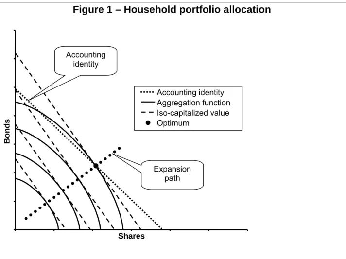
β β δ δ 1 ⎥⎦ ⎤ ⎢⎣ ⎡ ₊ = _w _A _t∗ _B _t∗ t A A B W [023]

with elasticity of transformation β τ − = 1 1 (β > 1) [024]

A few words about [023]. First, note that, if it were not for that constraint, all of the portfolio would be allocated to the asset with the highest rate of return in utility function [021]. Aggregation function [023], concave to the origin, imposes diversification (except in the particular case of corner solutions).

But accounting consistency requires that wealth constraint [022] be simultaneously satisfied. As demonstrated in Appendix 2, that implies

( )

[

]

( )

τ τ τ τ τ τ τ τ τ τ _δ _δ _δ δ − − − − − ⎭ ⎬ ⎫ ⎩ ⎨ ⎧ ₊ ₊ ₊ ⎭ ⎬ ⎫ ⎩ ⎨ ⎧ ₊ ₊ ₊ = 1 1 1 1 1 B1 1 t B A t A B t B A t A w i i i i A [025]

(19)

( )

⎭ ⎬ ⎫ ⎩ ⎨ ⎧ ₊ ₊ ₊ + = − − − ∗ τ τ τ τ τ τ δ δ δ B t B A t A A t A t t i i i W A 1 1 1 [026] and

( )

⎭ ⎬ ⎫ ⎩ ⎨ ⎧ ₊ ₊ ₊ + = − − − ∗ τ τ τ τ τ τ δ δ δ B t B A t A B t B t t i i i W B 1 1 1 [027]

The model can do without scale variable A_w.

Our formulation differs from the Decaluwé-Souissi model in two respects. First, A_t* and B_t* are the values of shares and bonds respectively, not their quantities . This implies that their prices are 1 by definition. Price variations appear as changes in rates of return, and are reflected in the value computation formulae applied to past issues (see 1.4 above, and 2.3 below). The second difference follows from the first : diversification constraint [023] is formulated in terms of asset values, rather than quantities.

3. ASSET MARKET EQUILIBRIUM

3.1 The supply of bonds

In each period, the supply of bonds consists of two components : the value of newly issued bonds, and that of bonds which were outstanding in the preceding period and do not come to maturity in the current period. New bonds are issued at a fixed price of 1; it is the current rate of interest which adjusts so as to equilibrate supply and demand5_{. As we have shown above, the} price of bonds issued in previous periods is adjusted according to the current rate of interest, so that bond-holders are indifferent between new bonds and those which were already outstanding. The aggregate value of still outstanding, previously issued bonds is computed with the adjusted prices in equation [018]6_.

The supply of new bonds is determined by the government’s financing needs. Net government financing needs are the difference between, on one hand, the total value of public investments

5 This is the exact opposite of Treasury bills, whose yield depends on the acquisition-price discount relative to its face value.

6 One can imagine that in every period, old bonds still outstanding are revalued according to [018], and then exchanged for an equal value of replacement bonds worth 1.

(20)

and redemption of debt coming to maturity in the current period, and, on the other hand, current government savings7_: t t t t t PKIG REMB SG B = + − Δ [028] where

IG_t is public investment in real terms in period t PK_t is the price of investment goods in period t SG_t is government savings in period t

It is not excluded a priori that the supply of new bonds be negative.

We make the simplifying assumption that public investments are a constant share of total investment : t IP t tIG IT PK =π [029]

where IT_t is total investment spending in period t, so that

t t t IP t IT REMB SG B = + − Δ π [030]

This simplifying assumption could easily be replaced by a more realistic specification, such as a public investment program (fixed exogenous values).

3.2 Stock market

In each period, the total value of shares offered consists of the value of newly issued shares, and shares issued in the past.

The value of new shares issued is equal to business financing requirements, which are the difference between private investment expenditure and business savings. Thus, we make the simplifying assumption that all private investment that is not financed out of business savings is financed by issuing new shares :

t t t t PKIE SE A = − Δ [031] where

IE_t is private investment in real terms in period t PK_t is the price of investment goods in period t SE_t is business savings in period t

(21)

Given [029],

(

_IP

)

_t t tIE IT PK = 1−π [032] and

(

_IP

)

_t _t t IT SE A = − − Δ 1 π [033]

It is not excluded a priori that the supply of new shares be negative.

3.3 Asset supply and demand equilibrium

Given that EXTER-Debt is developed essentially for illustrative purposes, and that we want to keep it as simple as possible, even at some cost in terms of realism, we make the following additional assumption. Foreign savings, equal to current account deficit CAB_t, are entirely dedicated to the purchase of shares; only the remainder, ΔA_t – CAB_t, is offered to households. In a CGE based on real data, the RoW would own a portfolio, just like households. The RoW’s portfolio would consist minimally of domestic shares and bonds, and of at least one foreign asset (labeled in a foreign currency). Model closure could then be modified. In EXTER-Debt, the current account deficit is fixed exogenously. But if the RoW owned a portfolio, the current account balance would be linked to the value of domestic assets which the RoW agrees to include in its portfolio, depending on the rate of return on the foreign asset : that foreign rate of return could then be fixed exogenously to close the model.

Given this additional simplifying assumption, household demand for shares must absorb the market value of shares already owned at the beginning of the period, A_t, plus newly issued shares, ΔA_t, minus foreign acquisition of shares, assumed to be equal to current account balance CAB_t. So we have

A_t* = A_t + ΔA_t – CAB_t [034] Whence, given [026],

( )

⎭ ⎬ ⎫ ⎩ ⎨ ⎧ ₊ ₊ ₊ + = − Δ + ₋ ₋ − τ τ τ τ τ τ δ δ δ B t B A t A A t A t t t t i i i W CAB A A 1 1 1 [035]

Household bond demand must absorb all supply of bonds, which consists of bonds issued in the current period (at face value), plus the value of bonds issued in the past and not coming to maturity in the current period. Hence,

(22)

B_t* = B_t + ΔB_t [036] and, given [027],

( )

⎭ ⎬ ⎫ ⎩ ⎨ ⎧ ₊ ₊ ₊ + = Δ + ₋ ₋ − τ τ τ τ τ τ δ δ δ B t B A t A B t B t t t i i i W B B 1 1 1 [037]

The interest rate adjusts in order to equilibrate the bond market.

3.4 Savings-investment equilibrium

Savings-investment equilibrium is characterized in our model by

t t t h ht t SM SE SG CAB IT =

∑

_, + + + [038]

That condition is automatically satisfied by asset market equilibrium. Indeed, given household asset demands [035] and [037],

t t t t t t B A A CAB W B +Δ + +Δ − = [039]

Substituting from household wealth constraint [019] results in

∑

+ + + = = − Δ + + Δ + h ht t t t t t t t t t B A A CAB W A B REMB SM B _, [040]

∑

+ = − Δ + Δ h ht t t t t A REMB CAB SM B _, [041]

Substituting the supply of new bonds [030] and shares [033], yields

[

+ −

]

+

[

(

−

)

−

]

− = +

_∑

h ht t t t t IP t t t

IPIT REMB SG 1 π IT SE REMB CAB SM ,

π [042]

which is equivalent to [038].

4. INVESTMENT DEMAND AND EQUILIBRIUM MECHANISM

4.1 Investment demand

Let

r_i,t be the rental rate of industry i’s capital in period t

tye be the (marginal) rate of taxation applied to capital income before depreciation, so the

(23)

δ_i be the rate of depreciation of industry i’s capital φ_t be the market discount rate applied in period t

Then the present value of the income stream generated by one unit of capital, beginning in t + 1 at r_i,t, and declining thereafter at a rate of δ_i per period, is equal to

(

)

(

)

i t t i t i t i i r tye r tye δ φ φ δ δ θ θ + − = − ⎟ ⎟ ⎠ ⎞ ⎜ ⎜ ⎝ ⎛ + − −

∑

∞ = , , 1 1 1 1 1 1 1 [043]

Now let PK_t be the replacement price of capital in period t, and

(

_t _i

)

t

t i PK

U_, = φ +δ [044]

is industry i’s user cost of capital in period t. Then

(

)

(

)

(

)

t i t i i t t t i U r tye PK r tye , , , 1 1 − = + − δ φ [045]

is the ratio of the market value to the replacement cost of a unit of capital, and it can be interpreted as Tobin’s « q ». Investment demand is specified following Jung and Thorbecke (2001)8_{as a constant elasticity increasing function of Tobin’s « q » :}

(

)

el indi t i t i i t i t i U r tye KD Id _ , , , , ₁ 1 ⎟⎟ ⎟ ⎠ ⎞ ⎜⎜ ⎜ ⎝ ⎛ − =γ [046]

It is acknowledged that this specification is at variance with Tobin’s theory. Indeed, according to the « q » theory, equilibrium investment is such that q equals 1.

Let the gross rate of return on capital in industry i, before depreciation, but net of taxes on capital income9_{, be}

(

)

t t i t i PK r tye _, , 1− = ρ [047]

and assume the expected return to be constant, equal to ρ_i,t (myopic expectations). Also define

8 Our specification differs from Jung-Thorbecke in that depreciation is taken into account in [044]. 9 This qualification is of no practical relevance in EXTER-Debt, where there are no such taxes.

(24)

∑

∞ = ∞ = ⎟ ⎟ ⎠ ⎞ ⎜ ⎜ ⎝ ⎛ + − − = ⎟ ⎟ ⎠ ⎞ ⎜ ⎜ ⎝ ⎛ + − − = + = = 1 1 , , 1 1 1 1 1 1 1 1 θ θ θ θ φ δ δ φ δ δ δ φ ζ t i i t i i i t t t i t i PK U [048]

The present value of a stream of income beginning in t + 1 at ζ_i,t, and declining thereafter at a rate of δ_i per period, discounted at rate φ_t, is equal to 1. So ζ_i,t is the rate of return required for the present value of the income stream generated by an investment in industry i to be equal to its cost when the market discount rate φ_t is applied.

From [047] and [048], investment demand [046] can be rewritten as

(

)

i el indi t i t i i ind el t i t i i t i t i U r tye KD Id _ , , _ , , , , ₁ 1 ₁ ⎟⎟ ⎟ ⎠ ⎞ ⎜⎜ ⎜ ⎝ ⎛ = ⎟⎟ ⎟ ⎠ ⎞ ⎜⎜ ⎜ ⎝ ⎛ − = ζ ρ γ γ [049]

The present value of the stream of income expected from new investment in industry i is larger or smaller than its cost (Tobin’s « q » is above or below 1), according to whether ρ_i,t is more or less than ζ_i,t.

Equilibrium between investment demand and total investment spending imposes the following constraint :

∑

= i it t t PK Id IT _, [050]

Note that the implicit assumption in the preceding equation is that public investment, which is a constant share of total investment according to [029], is distributed among industries together with private investment. This is another one of our simplifying assumptions, and it could easily be relaxed. We shall further assume that government receives shares for its contribution, like any other agent.

4.2 A closer look at the user cost of capital

4.2.1NEW SHARE ISSUES

Buyers of new shares in industry i will demand the market rate of return ζ_i,t. Specifically, new shareholders will demand a number of shares that will entitle them to a fraction of the income generated by the industry that will be sufficient for them to realize the yield they expect. So, to

(25)

raise new capital to finance investments of PK_t Id_i,t, the number of new shares issued will have to be

(

)

_i_t _i_t _i_t _t _i_t t i t i t i _tye_r _KD _PK _Id N N N , , 1 , , , , , ₁₋ ₌_ζ Δ + Δ + [051]

(

)

_i_t

[

(

_i

)

_i_t _i_t

]

_i_t _t _i_t t i t i t i _tye _r _KD _Id _PK _Id N N N , , , , , , , , ₁₋ ₁₋_δ ₊ ₌_ζ Δ + Δ [052]

where N_i,t is the number of shares outstanding at the beginning of the period, and ΔN_i,t the number of new shares issued.

Equation [052] reflects the view that, in accordance with the time structure adopted, income generated in the current period goes to those who were shareholders at the beginning of the period. Thus, when one purchases ownership of one unit of capital in industry i in period t, he/she will begin receiving income from period t + 1 onwards. So the left-hand side of [052] is the amount of income that will be paid to holders of the new shares in period t + 1, according to their share of ownership, assuming the rental price of capital r_i,t is the same as in the current period (myopic expectations). The right-hand side is the income they must receive for the present value of expected incomes to be equal to the value of the investment under myopic expectations. In other words, the number of shares issued must be such that the fraction of expected income attributed to the holders of new shares will produce the income they demand. Substitute

(

)

t t i t i PK r tye _, , 1− = ρ [047] and [052] becomes

(

)

[

_i _i_t _i_t

]

_i_t _t _i_t t t i t i t i t i Id PK Id KD PK N N N , , , , , , , , _ρ ₁₋_δ ₊ ₌_ζ Δ + Δ [053]

(

)

[

_i _i_t _i_t

]

_i_t _i_t t i t i t i t i Id Id KD N N N , , , , , , , , _ρ ₁₋_δ ₊ ₌_ζ Δ + Δ [054]

(

_i

)

i_it_t _i_t t i t i t i t i t i Id KD Id N N N , , , , , , , , 1− + = Δ + Δ δ ρ ζ [055]

(26)

So the equity owned by new investors is more or less than their contribution to the industry’s capital in t + 1 according to whether ζ_i,t is greater or smaller than ρ_i,t : if ζ_i,t is greater than ρ_i,t, new investment is financed by equity dilution; in the opposite case, there is equity enhancement.

So, for every dollar invested, the new shareholder receives an expected income stream of ζ_i,t in period t + 1, declining thereafter at the rate of δ_i. But the relevant rate for the portfolio manager is the rate of return net of depreciation, i_tA, which is defined implicitly by

(

)

1 1 1 1 1 , 1 1 = ⎟ ⎟ ⎠ ⎞ ⎜ ⎜ ⎝ ⎛ + − = +

∑

∞ = ∞ = _t it i A t t i ζ φ δ φ θ θ θ θ [056]

The present value of a constant stream of income of A t

i is equal to that of an expected income

stream of ζ_i,t in period t + 1, declining thereafter at the rate of δ_i. Since

(

φ_t

)

φ_t θ θ 1 1 1 1 = +

∑

∞ = [057] we substitute in [056] :

(

1

)

1 1 1 1 = = +

∑

∞ = A t t A t t i i φ φ θ θ [058] Therefore A t i = φ_t. [059]

The market rate of return which guides the portfolio manager in his/her choices, A t

i , is none

other than the market discount rate φ_t. It also follows from [044] and [048] that

(

)

(

A _i

)

t t i t t t i t t i PK PK PK i U_, = ζ _, = φ +δ = +δ [060]

The key role played by market rate of return A t

i in the savings-investment equilibrating

mechanism is now clear. Through user cost of capital U_i,t, any rise in A t

i dampens investment

(27)

[050]). A rise in A t

i also increases the fraction of the household portfolio dedicated to shares

(demand equation [026]), while reducing the market value of shares issued in the past already held in the portfolio A_t (equations [020] and [076]), and total household wealth [019]. The net effect on new share demand by households is nonetheless positive, as shown in Appendix 4).

4.2.2NEW AND OLD SHARE PRICES AND THE STOCK MARKET VALUATION OF CAPITAL

Since a number ΔN_i,t of new shares have been issued for a total amount of PK_t Id_i_,t, their unit

price is t i t i t N Id PK , , Δ [061]

As for the holders of shares outstanding at the beginning of the period, it follows from [052] that what they must give up to the new shareholders is ζ_i,t PK_t Id_i,t = U_i,t Id_i,, which is the user cost of the new capital, as it should. So, assuming myopic expectations, they expect to receive an income in period t + 1 of

(

)

[

_i _i_t _i_t

]

_i_t _t _i_t _t

{

_i_t

[

(

_i

)

_i_t _i_t

]

_i_t _i_t

}

t t i,PK 1 δ KD, Id, ζ , PK Id, PK ρ, 1 δ KD, Id, ζ, Id, ρ − + − = − + − [062]

(

)

[

_i _i_t _i_t

]

_i_t _t _i_t _t

[

_i_t

(

_i

)

_i_t

(

_i_t _i_t

)

_i_t

]

t t i,PK 1 δ KD, Id, ζ , PK Id, PK ρ, 1 δ KD, ρ, ζ , Id, ρ − + − = − + − [063]

In the following periods, that stream of income declines with depreciation. Since new and old shareholders are the same, their discount rates are the same : A

t

i = φ_i,t. So the present value of

the stream of income that old shareholders expect to receive is equal to :

(

)

A t

[

it

(

i

)

it

(

it it

)

it

]

t i i Id KD PK i , , , , , 1 1 1 1 1 1 δ _ρ _δ _ρ _ζ δ θ θ − + − ⎟ ⎟ ⎠ ⎞ ⎜ ⎜ ⎝ ⎛ + − −

∑

∞ =

(

)

(

)

[

_i_t _i _i_t _i_t _i_t _i_t

]

t i A t Id KD PK i , , , , , 1 1 _ρ _δ _ρ _ζ δ − + − + = [064]

(

)

(

)

[

_i_t _i _i_t _i_t _i_t _i_t

]

t t i Id KD PK _, _, _, _, _, , 1 1 _ρ _δ _ρ _ζ ζ − + − = [065]

(28)

(

)

⎥ ⎥ ⎦ ⎤ ⎢ ⎢ ⎣ ⎡ ⎟ ⎟ ⎠ ⎞ ⎜ ⎜ ⎝ ⎛ − + − = _i_t t i t i t i i t i t i t KD Id PK _, , , , , , ₁ ₁ ζ ρ δ ζ ρ [066] ⎥ ⎥ ⎦ ⎤ ⎢ ⎢ ⎣ ⎡ − = ₊ t i t i t i t i t KD Id PK _, ₁ _, , , ζ ρ [067]

The unit price of old shares is their value, divided by their number :

⎥ ⎥ ⎦ ⎤ ⎢ ⎢ ⎣ ⎡ − + it t i t i t i t t _KD _Id N PK , 1 , , , ζ ρ

It is demonstrated in the following box that the price of old shares is identical to the price of new ones. So share pricing is perfectly compatible with the fact that new and old shareholders are the same agent.

Demonstration of the equality of prices between old and new shares : From [055], the number of new shares is

(

)

(

it it

)

t i t i i t i t i t i t i N N Id KD Id N _, _, , , , , , , 1− + +Δ = Δ δ ρ ζ [068]

(

)

(

)

it t i t i i t i t i t i t i t i t i i t i t i t i _N Id KD Id N Id KD Id , , , , , , , , , , , , 1 1 1 + − = Δ ⎟⎟ ⎟ ⎠ ⎞ ⎜⎜ ⎜ ⎝ ⎛ + − − δ ρ ζ δ ρ ζ [069]

(

)

(

)

t i t i t i i t i t i t i t i t i i t i t i t i t i N Id KD Id Id KD Id N _, , , , , , , , , , , , 1 1 1 ⎟⎟ ⎟ ⎠ ⎞ ⎜⎜ ⎜ ⎝ ⎛ + − − ⎟⎟ ⎟ ⎠ ⎞ ⎜⎜ ⎜ ⎝ ⎛ + − = Δ δ ρ ζ δ ρ ζ [070]

(

)

it t i t i t i i t i t i t i N Id Id KD N _, , , , , , , 1 1 1 ⎟⎟ ⎟ ⎠ ⎞ ⎜⎜ ⎜ ⎝ ⎛ − + − = Δ δ ζ ρ [071]

(29)

(

)

⎟⎟ ⎟ ⎠ ⎞ ⎜⎜ ⎜ ⎝ ⎛ − + − = Δ 1 1 , , , , , , , , , t i t i t i i t i t i t i t i t t i t i t Id Id KD N Id PK N Id PK δ ζ ρ [072]

(

)

[

]

⎟⎟ ⎟ ⎠ ⎞ ⎜⎜ ⎜ ⎝ ⎛ − + − = Δ _i_t i it it it t i t i t t i t i t Id Id KD N PK N Id PK , , , , , , , , ₁ _δ ζ ρ [073] ⎟⎟ ⎟ ⎠ ⎞ ⎜⎜ ⎜ ⎝ ⎛ − = Δ it+ it t i t i t i t t i t i t Id KD N PK N Id PK , 1 , , , , , , ζ ρ [074]

which is precisely the price of old shares. Q.E.D.

Since the price of old and new shares is the same, the total stock market value of industry i in period t is simply 1 , , , , , 1 , , , , , , , + + _⎟⎟ = ⎠ ⎞ ⎜ ⎜ ⎝ ⎛ − + Δ Δ it t i t i t t i t i t i t i t i t i t t i t i t i t KD PK N Id KD N PK N N Id PK ζ ρ ζ ρ [075]

Note that the current stock market value of an industry is different from the market value of its currently productive capital, since the stock market value is forward looking in that it includes the value of current investments which come on line only in the following period, and takes into account end-of-period depreciation. But the stock market value is forward looking in a simplistic way, since it is based on myopic expectations relative to replacement price of capital PK_t₊₁, and return rates ρ_i,t₊₁ and ζ_i,t₊₁.

The second term on the left-hand side of [075] is the current stock market value of shares issued in the past :

(

)

∑

_⎥⎥ ⎦ ⎤ ⎢ ⎢ ⎣ ⎡ ⎟ ⎟ ⎠ ⎞ ⎜ ⎜ ⎝ ⎛ − + − = i it it t i t i i t i t i t t PK KD Id WK _, , , , , , ₁ ₁ ζ ρ δ ζ ρ [076]

4.2.3OWNERSHIP AND DIVIDEND DISTRIBUTION

Contrary to stock market value, dividend distribution is, so to speak, backward looking : capital income is generated by currently productive capital, which consists of depreciated capital that was already productive, and investments made in the preceding period.

(30)

So the fraction of current capital income generated in industry i that belongs to those who invested in the previous period is

1 , 1 , 1 , − − − Δ + Δ t i t i t i N N N

The fraction of ownership attributed to new shares issued in period t–1, according to [055], corresponds to the whole amount of investment. But part of that was financed by business savings, retained earnings of the previous period, which were not distributed as dividends. So the corresponding fraction of ownership must be distributed proportionately to dividend entitlements in the previous period. Therefore, given that the fraction of investment finances out of retained earnings in period t–1 is

1 1 − − t t IT SE

, the ownership fraction of agent j in the capital of industry i during period t is therefore

1 , 1 , 1 , 1 1 1 , 1 , 1 , 1 , 1 1 1 , 1 , 1 , 1 , 1 − − − − − − − − − − − − − − − ₊_Δ Δ ⎟ ⎟ ⎠ ⎞ ⎜ ⎜ ⎝ ⎛ − + ⎟ ⎟ ⎠ ⎞ ⎜ ⎜ ⎝ ⎛ Δ + Δ + Δ + _i_t _i_t t i t t I t j t i t i t i t t t i t i t i K t j _N _N N IT SE N N N IT SE N N N λ λ [077]

where it is assumed that, in period t–1, the ownership fraction of a given agent was the same in all industries (as if the shares of all industries were pooled in a single mutual fund), and where

I t j,−1

λ is the fraction acquired by agent j in the new shares issued in period t–1 that correspond to the part of investment not financed out of retained earnings ( I

t j,−1

λ is also assumed to be equal across industries).

To be consistent with our simplifying assumption that public investment funding is pooled with private funding (equations [029] and [050]), the government is also a shareholder, whose purchases of new shares are equal to public investment expenditures :

1 1 1 1 , − − − − = ₋ t t t IP I t G _IT _SE IT π λ [078]

And, consistent with [034], the RoW’s share in investments is

1 1 1 1 , − − − − = ₋ t t t I t RoW _IT _SE CAB λ [079]

Finally, the households’ share is

I t G I t RoW I t H, 1 λ , λ , λ = − − [080]

(31)

The ownership fraction of agent j in the capital of all industries (in the all-industries mutual fund),

K t j,

λ , is the weighted sum of industry fractions [077]. It is demonstrated in Appendix 3 that

(

)

(

)

1 1 , 1 1 1 , 1 1 , 1 , , − − − − − − − − + − + + = t t i t t I t j t t i K t j K t j _WK _IT SE IT SE WK λ λ λ [081]

5. SIMULATION EXPERIMENTS WITH EXTER-DEBT

5.1 Calibration

In the version presented here, EXTER-Debt calibrated with the objective that, in the absence of shocks, it follow a regular path, that is, a path of balanced growth, at a rate equal to exogenous population growth n.

A necessary condition to achieve that purpose, is that exogenous flows all grow at rate n : • labor supply

(

)

_t t nLS

LS₊₁= 1+ [082]

• public transfers to households (except interests paid on the public debt, which are endogenous)

(

)

_h_t t h nTG TG _,₊₁ = 1+ _, [083] • government spending

(

)

_t t nG G₊₁= 1+ [084]

• the current account balance

(

)

_t t nCAB

CAB ₊₁= 1+ [085]

A second requirement is that past bond issues must have grown at the demographic growth rate

n, so that the amount to be redeemed may grow at the same rate in the future. Government

savings depend on the amount of interests paid on outstanding bonds, which in turn depends on the history of bond issues. For interest payments on the public debt to grow at rate n, with amounts issued also growing at rate n, past period interest rates must have been equal to the current base period rate. Finally, given the amount of government savings, and a current issue of new bonds equal to n+1 times that of the previous period, public investment is set accordingly. It must also be taken into account that investment expenditures depend, among others, on household savings, and therefore on interest payments on the public debt.

(32)

A further requirement of a regular path is that the capital stock and investment demand functions be calibrated so that, coeteris paribus, the capital stock of every industry grows at rate

n. Moreover, the initial capital ownership shares of agents were set equal to their respective

contributions to investment in the base period so that ownership shares remain constant. The initial rate of return on shares was set equal to the weighted average rate of return to capital, net of taxes and depreciation.

It was not easy to engineer a SAM with all the required characteristics. And, as we shall see later on, although these characteristics are necessary conditions for the economy to follow a regular path, they are not quite sufficient.

5.2 Simulations

5.2.1QUASI-REGULAR PATH

We have run our model without shock for 30 periods. We observe that the period-to-period change in flow variables is indeed very close to the 1% demographic rate of growth stipulated. But not exactly. And most price variables change very little. But they do. So our results reveal that the path followed by the economy is not quite regular.

Why? Among the price variables that do change significantly is the rate of interest. After 30 periods, the rate of return on shares, irac, is practically unchanged (+0.33% relative to its base period value), while interest rate ir has increased by more than 55%. That is because our calibration procedure has not taken into account the initial proportion of shares and bonds in the households’ portfolio. Now, the ratio of the value of new to old bonds in the portfolio is far larger than that of new to old shares. So the proportion of each type of asset in the portfolio changes progressively in favor of bonds, which exerts pressure on the interest rate : households are persuaded to increase the proportion of bonds in their portfolio only if they are offered a higher rate of interest.

It is not so easy as it would seem at first sight to imagine numbers that would correct that situation. First, for new issues to grow at rate n, any increase in the stock of previously issued bonds implies a proportional increase of the issue of new bonds in the base period : consequently, this is no way to move the rates of increase of the two portfolio components closer to one another. As for modifying the value of A_t, shares issued in previous periods in the household portfolio, it is precluded by the tight relationship between A_t and WK_t (equation [020]), and by the fact that the latter is entirely determined by previously calibrated variables

(33)

(see A5.3 in Appendix 5). Finally, modifying the amount of new shares issued is equivalent to constructing a whole new SAM.

In view of these difficulties, we shall be content with a quasi-regular path.

5.2.2ZERO-GROWTH SCENARIO

Before proceeding with counter-factual simulations departing from the quasi-regular path, the model was further tested to see if it could reproduce a stationary state, i.e. a situation in which the base-period values are repeated from period to period, indefinitely. Basically, the necessary conditions are the same as for the quasi-regular path, except that the growth rate n is set to zero.

This exercise required constructing a new SAM, because of changes in the history of past bond issues. For a stationary state to prevail, past issues must have been of equal amounts every period. And that implies that new bonds are currently issued for an amount exactly equal to current redemption of bonds coming to maturity; this differs from the quasi-regular SAM, where the amount of newly issued bonds is n+1 times the redemption of mature bonds. It follows that public investment is equal to government savings. So adjustments cascade throughout the SAM. To facilitate the construction of the steady-state SAM, dividend distribution parameters were disconnected from ownership fractions, and simply set equal to initial values.

Apart from that, and starting from a different SAM, the zero-growth version of EXTER-Debt is identical to the other one10_{. And, as expected, the base-period values are repeated from period} to period, indefinitely.

5.2.3DOUBLING THE SHARE OF PUBLIC INVESTMENTS

The BAU scenario is the quasi-regular path described above. The shock is applied in the second period. The amount of new bonds issued immediately increases by more than 80%, while there are consequently less new shares issued. In order for the households to absorb the abundance of new bonds, the rate of interest jumps from 1% to nearly 2.5%. As a result, interest payments begin to increase in the following, third, period. Government savings show a modest increase in the third period, a paradox which disolves when it is realized that the increase in public investment augments the government ownership fraction, and therefore the amount of dividends it receives. But that effect is quickly overwhelmed, beginning in the fourth period, by

Bond Indebtedness in a Recursive Dynamic CGE Model

Cahier de recherche/Working Paper 07-10