Université de Montréal
Deep Neural Networks for Natural Language Processing
and its Acceleration
par
Zhouhan Lin
Département d’informatique et operational recherche Faculté des arts et des sciences
Thèse présentée à la Faculté des études supérieures et postdoctorales en vue de l’obtention du grade de
Philosophiæ Doctor (Ph.D.) en Informatique
août 2019
c
Sommaire
Cette thèse par article comprend quatre articles qui contribuent au domaine de l’apprentissage profond, en particulier à l’accélération de l’apprentissage par le biais de réseaux à faible précision et à l’application de réseaux de neurones profonds au traitement du langage naturel.
Dans le premier article, nous étudions un schéma d’entraînement de réseau de neurones qui élimine la plupart des multiplications en virgule flottante. Cette approche consiste à binariser ou à ternariser les poids dans la propagation en avant et à quantifier les états cachés dans la propagation arrière, ce qui convertit les multiplications en changements de signe et en décalages binaires. Les résultats expérimentaux sur des jeux de données de petite à moyenne taille montrent que cette approche produit des performances encore meilleures que l’approche standard de descente de gradient stochastique, ouvrant la voie à un entraînement des réseaux de neurones rapide et efficace au niveau du matériel.
Dans le deuxième article, nous avons proposé un mécanisme structuré d’auto-attention d’enchâssement de phrases qui extrait des représentations interprétables de phrases sous forme matricielle. Nous démontrons des améliorations dans 3 tâches différentes: le profilage de l’auteur, la classification des sentiments et l’implication textuelle. Les résultats expéri-mentaux montrent que notre modèle génère un gain en performance significatif par rapport aux autres méthodes d’enchâssement de phrases dans les 3 tâches.
Dans le troisième article, nous proposons un modèle hiérarchique avec graphe de calcul dynamique, pour les données séquentielles, qui apprend à construire un arbre lors de la lec-ture de la séquence. Le modèle apprend à créer des connexions de saut adaptatives, ce qui facilitent l’apprentissage des dépendances à long terme en construisant des cellules récur-rentes de manière récursive. L’entraînement du réseau peut être fait soit par entraînement
supervisée en donnant des structures d’arbres dorés, soit par apprentissage par renforce-ment. Nous proposons des expériences préliminaires dans 3 tâches différentes: une nouvelle tâche d’évaluation de l’expression mathématique (MEE), une tâche bien connue de la logique propositionnelle et des tâches de modélisation du langage. Les résultats expérimentaux mon-trent le potentiel de l’approche proposée.
Dans le quatrième article, nous proposons une nouvelle méthode d’analyse par circon-scription utilisant les réseaux de neurones. Le modèle prédit la structure de l’arbre d’analyse en prédisant un scalaire à valeur réelle, soit la distance syntaxique, pour chaque position de division dans la phrase d’entrée. L’ordre des valeurs relatives de ces distances syntax-iques détermine ensuite la structure de l’arbre d’analyse en spécifiant l’ordre dans lequel les points de division seront sélectionnés, en partitionnant l’entrée de manière récursive et de-scendante. L’approche proposée obtient une performance compétitive sur le jeu de données Penn Treebank et réalise l’état de l’art sur le jeu de données Chinese Treebank.
Mots-clés: réseaux neuronaux quantifiés, connexion ternaire, connexion binaire, enchâssement de phrase, auto-attention, inférence en langage naturel, analyse des sen-timents, graphe de calcul dynamique, réseaux récurrents, analyse syntaxique, analyseur syntaxique, réseaux neuronaux, apprentissage profond, langage naturel traitement, apprentissage automatique
Summary
This thesis by article consists of four articles which contribute to the field of deep learning, specifically in the acceleration of training through low-precision networks, and the application of deep neural networks on natural language processing.
In the first article, we investigate a neural network training scheme that eliminates most of the floating-point multiplications. This approach consists of binarizing or ternarizing the weights in the forward propagation and quantizing the hidden states in the backward propagation, which converts multiplications to sign changes and binary shifts. Experimental results on datasets from small to medium size show that this approach result in even better performance than standard stochastic gradient descent training, paving the way to fast, hardware-friendly training of neural networks.
In the second article, we proposed a structured self-attentive sentence embedding that extracts interpretable sentence representations in matrix form. We demonstrate improve-ments on 3 different tasks: author profiling, sentiment classification and textual entailment. Experimental results show that our model yields a significant performance gain compared to other sentence embedding methods in all of the 3 tasks.
In the third article, we propose a hierarchical model with dynamical computation graph for sequential data that learns to construct a tree while reading the sequence. The model learns to create adaptive skip-connections that ease the learning of long-term dependencies through constructing recurrent cells in a recursive manner. The training of the network can either be supervised training by giving golden tree structures, or through reinforcement learning. We provide preliminary experiments in 3 different tasks: a novel Math Expression Evaluation (MEE) task, a well-known propositional logic task, and language modelling tasks. Experimental results show the potential of the proposed approach.
In the fourth article, we propose a novel constituency parsing method with neural net-works. The model predicts the parse tree structure by predicting a real valued scalar, named syntactic distance, for each split position in the input sentence. The order of the relative values of these syntactic distances then determine the parse tree structure by specifying the order in which the split points will be selected, recursively partitioning the input, in a top-down fashion. Our proposed approach was demonstrated with competitive performance on Penn Treebank dataset, and the state-of-the-art performance on Chinese Treebank dataset. Keywords: quantized neural networks, ternary connect, binary connect, sentence em-bedding, self-attention, natural language inference, sentiment analysis, dynamic computa-tional graph, recurrent networks, recursive networks, constituent parsing, syntactic parser, neural networks, deep learning, natural language processing, machine learning
Contents
Sommaire . . . iii
Summary . . . v
List of tables . . . xiii
List of figures . . . xv
Acknowledgement . . . xix
Chapter 1. Machine Learning Backgrounds . . . 1
1.1. Machine Learning . . . 1
1.2. Types of Learning . . . 2
1.3. Parametric and Non-parametric Models . . . 4
1.4. Maximum Likelihood Estimation . . . 5
1.5. Generalization and Model Capacity . . . 6
1.6. Parameters and Hyperparameters . . . 8
1.7. Regularization . . . 8
Chapter 2. Neural Networks . . . 11
2.1. Convolutional Neural Networks . . . 11
2.2. Recurrent Neural Networks . . . 13
2.2.1. Vanilla Recurrent Networks . . . 14
2.2.3. Gated Recurrent Unit . . . 17
2.3. Attention Mechanism . . . 18
2.4. Transformer . . . 20
2.5. Low-precision neural networks . . . 24
2.5.1. Multiplication . . . 24
2.5.2. Memory Demand . . . 25
Chapter 3. Natural Language Processing . . . 27
3.1. Encoding words: Neural Language Models . . . 27
3.2. Encoding sentences: Sentence Embeddings . . . 30
3.3. Contextualized Pre-trained Models . . . 33
Chapter 4. Prologue to First Article . . . 35
4.1. Article Details . . . 35
4.2. Context . . . 35
4.3. Contributions . . . 36
4.4. Recent Developments . . . 36
Chapter 5. Neural Networks with Few Multiplications . . . 37
5.1. Introduction . . . 37
5.2. Related work . . . 37
5.3. Binary and ternary connect . . . 38
5.3.1. Binary connect revisited . . . 38
5.3.2. Ternary connect . . . 39
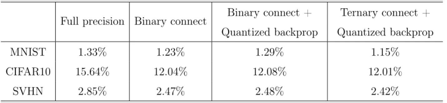
5.5. Experiments . . . 42 5.5.1. General performance . . . 42 5.5.1.1. MNIST . . . 43 5.5.1.2. CIFAR10 . . . 44 5.5.1.3. SVHN . . . 44 5.5.2. Convergence . . . 45
5.5.3. The effect of bit clipping . . . 45
5.6. Conclusion and future work . . . 46
Chapter 6. Prologue to Second Article . . . 49
6.1. Article Details . . . 49
6.2. Context . . . 49
6.3. Contributions . . . 50
6.4. Recent Developments . . . 50
Chapter 7. A Structured Self-Attentive Sentence Embedding . . . 51
7.1. Introduction . . . 51 7.2. Approach . . . 52 7.2.1. Model . . . 52 7.2.2. Penalization term . . . 55 7.2.3. Visualization . . . 56 7.3. Related work . . . 57 7.4. Experimental results . . . 58 7.4.1. Author profiling . . . 58 7.4.2. Sentiment analysis . . . 59 7.4.3. Textual entailment . . . 62 7.4.4. Exploratory experiments . . . 63
7.4.4.1. Effect of penalization term . . . 63
7.4.4.2. Effect of multiple vectors. . . 65
7.5. Conclusion and discussion . . . 65
7.6. Pruned MLP for Structured Matrix Sentence Embedding . . . 67
7.7. Detailed Structure of the Model for SNLI Dataset . . . 69
Chapter 8. Prologue to Third Article . . . 73
8.1. Article Details . . . 73
8.2. Context . . . 73
8.3. Contributions . . . 74
8.4. Recent Developments . . . 74
Chapter 9. Learning Hierarchical Structures on the Fly with a Recurrent-Recursive Model for Sequences . . . 75
9.1. Introduction . . . 75 9.2. Model . . . 77 9.3. Experimental Results . . . 78 9.3.1. Math Induction . . . 78 9.3.2. Logical inference . . . 81 9.3.3. Language Modeling . . . 81 9.4. Final Considerations . . . 82
Chapter 10. Prologue to Fourth Article . . . 83
10.1. Article Details . . . 83
10.2. Context . . . 83
10.4. Recent Developments . . . 84
Chapter 11. Straight to the Tree: Constituency Parsing with Neural Syntactic Distance . . . 85
11.1. Introduction . . . 85
11.2. Syntactic Distances of a Parse Tree . . . 87
11.3. Learning Syntactic Distances. . . 90
11.3.1. Model Architecture . . . 90 11.3.2. Objective . . . 92 11.4. Experiments . . . 93 11.4.1. Penn Treebank . . . 94 11.4.2. Chinese Treebank . . . 95 11.4.3. Ablation Study . . . 97 11.5. Related Work . . . 97 11.6. Conclusion . . . 98 Chapter 12. Conclusion . . . 101 Bibliography . . . 103
List of tables
5.1 Performances across different datasets . . . 42
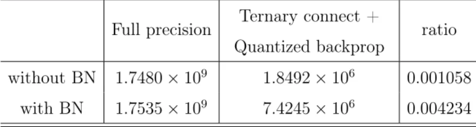
5.2 Estimated number of multiplications in MNIST net . . . 44
7.1 Performance Comparison of Different Models on Yelp and Age Dataset . . . 58
7.2 Test Set Performance Compared to other Sentence Encoding Based Methods in SNLI Datset . . . 61
7.3 Performance comparision regarding the penalization term . . . 65
7.4 Model Size Comparison Before and After Pruning . . . 68
9.1 Sample expressions from MEE dataset . . . 79
9.2 Prediction accuracy on MEE dataset. . . 80
11.1 Results on the PTB dataset WSJ test set, Section 23. LP, LR represents labeled precision and recall respectively. . . 94
11.2 Test set performance comparison on the CTB dataset . . . 96
11.3 Detailed experimental results on PTB and CTB datasets . . . 96
11.4 Ablation test on the PTB dataset. “w/o top LSTM” is the full model without the top LSTM layer. “w Char LSTM” is the full model with the extra Character-level LSTM layer. “w. embedding” stands for the full model using the pretrained word embeddings. “w. MSE loss” stands for the full model trained with MSE loss. . . 97
List of figures
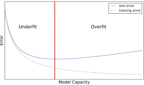
1.1 An illustration of underfit and overfit with respect to the change on model capacity. The vertical read line corresponds to the optimal model capacity, which corresponds to the minimum in test error. . . 7
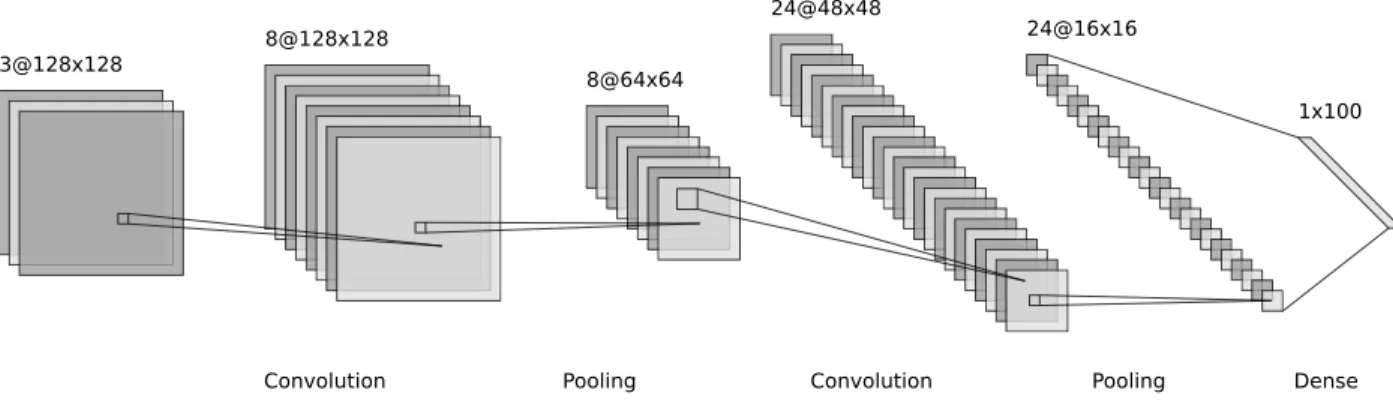
2.1 A typical structure of convolutional neural networks. The first pile of rectangles (3@128x128) stands for the original image, with its 3 channels standing for RGB channels. The latter piles of rectangles stand for the hidden states in the convolutional network, with the size of the pile being the number of channels, and the size of the rectangles in the piles stand for the shape of the hidden states. The last layer is a dense layer with flat outputs, which represented by a long rectangle strip to the right of the figure. . . 12
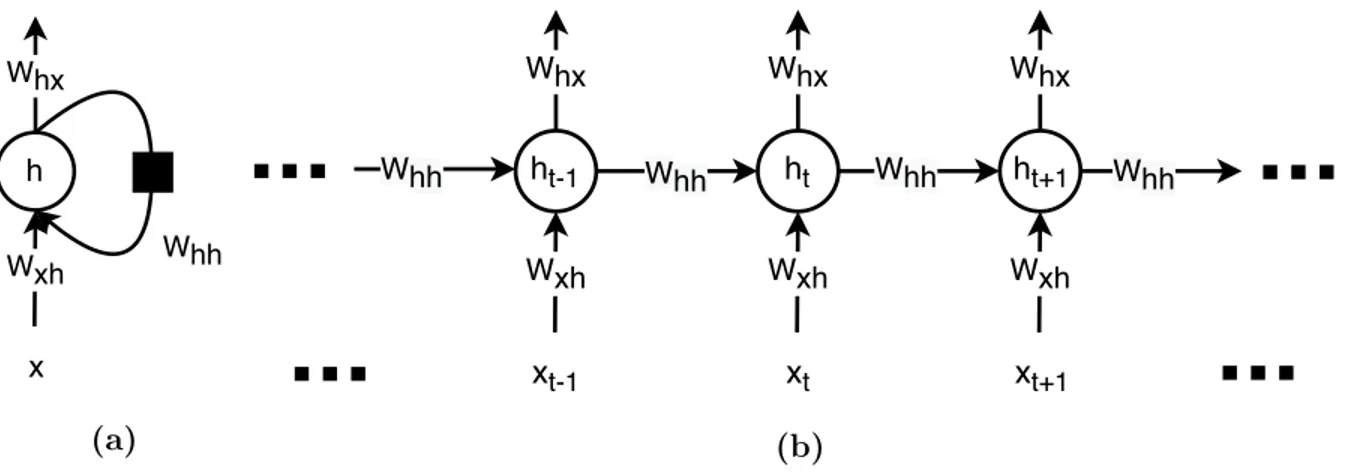
2.2 Structure of a simple single layer, unidirectional recurrent neural network. (a) The folded diagram of the RNN, showing its structure as a directed cyclic graph. The black rectangle stands for a one step time delay. (b) The unfolded diagram of the same RNN, which unfolds the RNN in the time direction by repeatedly drawing the same cell over all time steps. The unfolded structure should always be acyclic. 15
2.3 Structure of bidirectional recurrent neural network. For simplicity we omitted all the notations on weights and hidden states. . . 16
2.4 Attention mechanism in a machine translation context. The upper unidirectional RNN is a decoder that is trying to infer the next word yj, and the lower
bidirectional RNN is an encoder that encodes source sentence tokens into a sequence of hidden states. . . 19
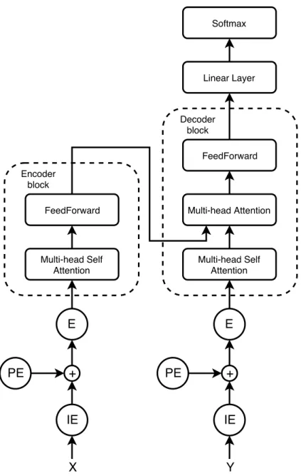
2.5 Structure of the Transformer model. For simplicity we merge all the individual tokens in a sequence and represent them as a whole, which is notated as X and Y
in the figure. Within each of the components in the encoder and decoder block, there is a layer normalization step included. Please refer to the text for details. . 21
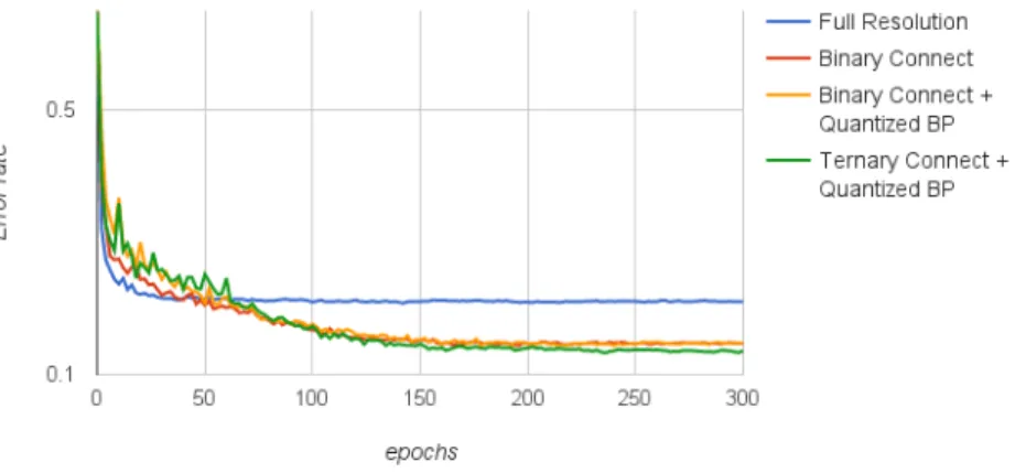
5.1 Test set error rate at each epoch for ordinary back propagation, binary connect, binary connect with quantized back propagation, and ternary connect with quantized back propagation. Vertical axis is represented in logarithmic scale. . . 45
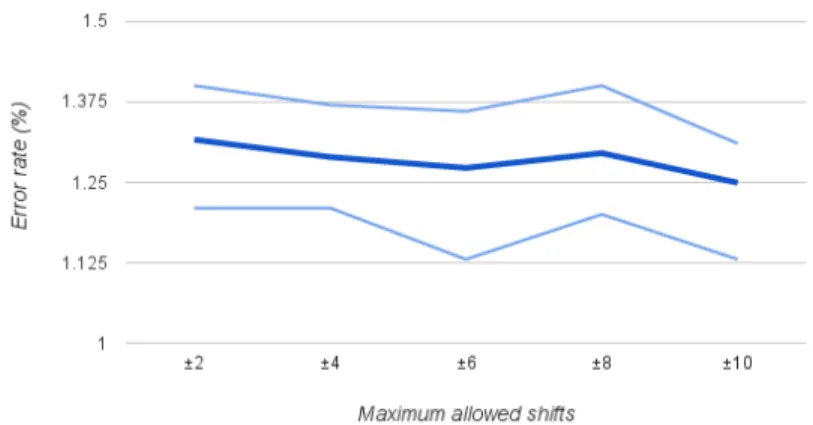
5.2 Model performance as a function of the maximum bit shifts allowed in quantized back propagation. The dark blue line indicates mean error rate over 10 independent runs, while light blue lines indicate their corresponding maximum and minimum error rates. . . 46
5.3 Histogram of representations at each layer while training a fully connected network for MNIST. The figure represents a snap-shot in the middle of training. Each subfigure, from bottom up, represents the histogram of hidden states from the first layer to the last layer. The horizontal axes stand for the exponent of the layers’ representations, i.e., log2x. . . 47 7.1 A sample model structure showing the sentence embedding model combined with
a fully connected and softmax layer for sentiment analysis (a). The sentence embedding M is computed as multiple weighted sums of hidden states from a bidirectional LSTM (h1, ..., hn), where the summation weights (Ai1, ..., Ain) are
computed in a way illustrated in (b). Blue colored shapes stand for hidden representations, and red colored shapes stand for weights, annotations, or input/output. . . 53
7.2 Heatmap of Yelp reviews with the two extreme score. . . 60
7.3 Heat maps for 2 models trained on Age dataset. The left column is trained without the penalization term, and the right column is trained with 1.0 penalization. (a) and (b) shows detailed attentions taken by 6 out of 30 rows of the matrix embedding, while (c) and (d) shows the overall attention by summing up all 30 attention weight vectors. . . 64
7.4 Attention of sentence embedding on 3 different Yelp reviews. The left one is trained without penalization, and the right one is trained with 1.0 penalization. . 64
7.5 Effect of the number of rows (r) in matrix sentence embedding. The vertical axes indicates test set accuracy and the horizontal axes indicates training epochs. Numbers in the legends stand for the corresponding values of r. (a) is conducted in Age dataset and (b) is conducted in SNLI dataset. . . 66
7.6 Hidden layer with pruned weight connections. M is the matrix sentence embedding, Mv and Mh are the structured hidden representation computed
by pruned weights. . . 68
7.7 Model structure used for textual entailment task. . . 70
9.1 (a) - (c) are the 3 different cells. (d) is a sample model structure resulted from a sequence of decisions. "R", "S" and "M" stand for recurrent cell, split cell, and merge cell, respectively. Note that the "S" and "M" node can take inputs in datasets where splitting and merging signals are part of the sequence. (e) is the tree inferred from (d). . . 75
9.2 Test accuracy of the models, trained on sequences of length ≤ 6 in logic data. The horizontal axis indicates the length of the sequence, and the vertical axis indicates the accuracy of model’s performance on the corresponding test set. . . 80
11.1 An example of how syntactic distances (d1 and d2) describe the structure of a parse tree: consecutive words with larger predicted distance are split earlier than those with smaller distances, in a process akin to divisive clustering. . . 86
11.2 Inferring the parse tree with Algorithm 3 given distances, constituent labels, and POS tags. Starting with the full sentence, we pick split point 1 (as it is assigned to the larger distance) and assign label S to span (0,5). The left child span (0,1) is assigned with a tag PRP and a label NP, which produces an unary node and a terminal node. The right child span (1,5) is assigned the label ∅, coming from implicit binarization, which indicates that the span is not a real constituent and
all of its children are instead direct children of its parent. For the span (1,5), the split point 4 is selected. The recursion of splitting and labeling continues until the process reaches a terminal node. . . 88
11.3 The overall visualization of our model. Circles represent hidden states, triangles represent convolution layers, block arrows represent feed-forward layers, arrows represent recurrent connections. The bottom part of the model predicts unary labels for each input word. The ∅ is treated as a special label together with other labels. The top part of the model predicts the syntactic distances and the constituent labels. The inputs of model are the word embeddings concatenated with the POS tag embeddings. The tags are given by an external Part-Of-Speech tagger. . . 91
Acknowledgement
There are a lot of people who helped me in various aspects of the research I conducted, as well as being supportive during the past five years.
I’d especially like to thank my supervisor, Yoshua Bengio, for taking me onto the boat of deep learning, and for his supervision on my research. His insights towards various research fields have always shed light on my vision towards the problems in those fields. His perse-verance and enthusiasm have encouraged me as well. I’d also like to thank him for always keeping the Mila lab an open, inclusive, and collaborative research lab. It provides such a great environment that allows students, professors, and even external collaborators to freely explore various ideas out of their curiosity. I’d also like to thank Roland Memisevic, who was also my supervisor and worked with me in my early days of Ph.D. study.
I’d also like to thank all of my collaborators without whom this thesis won’t be possible. Specifically, I’d like to thank Aaron Courville for his discussions and advise. Alessandro Sordoni for hosting me at Microsoft Research Montreal, and provides precious feedback and critiques on my proposed research. Yikang Shen for the close collaboration, and the discussions and debates we had. Athul Paul Jacob for the work we’ve done together at Microsoft Research Montreal. Matthieu Courbariaux for the collaborations on low precision networks. Minwei Feng, Mo Yu, Bowen Zhou and Bing Xiang for the work we’ve done at IBM. Also, I’d like to thank Samuel Lavoie for translating the summary in this thesis into French for me.
There are several people who were supportive to my life outside of research. I’d like to thank Kyunghyun Cho for always organizing those beer parties when he was here, which helped me get involved into the lab more quickly. Athul Paul Jacob for always keeping his pranks happening in its surprising way. Shawn Tan for his memes, jokes, and his extended
vocabulary in multiple languages that make us happy, even when facing tightest deadlines. Cheng Li and Guoxin Gu for the various kinds of sports we had played together.
There are also a lot of people I want to thank, who helped me in various ways. These include Jie Fu, Jian Tang, Jae Hyun Lim, Min Lin, Ziwei He, Sarath Chandar, Dmitriy Serdyuk, Sandeep Subramanian, Vincent Michalski, Julian Vlad Serban, Dendi Suhubdy, Chinnadhurai Sankar, Chin-Wei Huang, Mathieu Germain, Saizheng Zhang, Dong-Hyun Lee, Yuhuai Wu, Joachim Ott, Ying Zhang, Adam Trischler, Frederic Bastien, and Guillaume Alain.
Lastly, I would like to thank my mother, my aunt, and my grand parents for their support during my academic career.
Chapter 1
Machine Learning Backgrounds
This thesis focuses on several topics around deep learning, which is a machine learning approach based on neural networks. We’ll provide some background knowledge in machine learning and neural networks in this chapter, and in subsequent chapters we are going to dive deep into more specific topics that are related to the work being introduced in the thesis. The remainder of the thesis presents the articles. For the articles to be presented, we will first introduce low precision networks. Then we will introduce an early version of self attention which is used in sentiment analysis and natural language inference. Finally we will introduce a neural parser where a neural network is used to learn grammar trees out from its hidden states.
In this chapter I will give a brief introduction to some of the important basic aspects and concepts of machine learning that will be used and studied in the subsequent chapters. As supervised learning will be studied a lot in subsequent articles, I will use this learning scheme as a main example while introducing various machine learning concepts. More details on other learning schemes and the concepts being introduced here can be found in [13] and [51].
1.1. Machine Learning
Machine learning is a sub-field in computer science that seeks to enable computer systems to learn knowledge through data, observations, and interactions with the world. The acquired knowledge should be general enough so that it also allows the computer systems to correctly generalize to new observations or even new settings.
Seen as a subset of a much broader field named artificial intelligence, machine learning is of important merits in both theoretical and practical aspects. Theoretically it has developed
into several branches in theoretical computer science, such as computational learning theory and statistical learning theory. Practically, benefiting from the increase in data production and computational power, the recent resurgence of the neural network approach has revo-lutionized, and become the dominant technical approach, in a wide variety of application fields, such as computer vision [93], speech recognition [65], and natural language processing [5]. These achievements in the past several decades has made machine learning an important part of computer science.
Early in the 1950s Alan Turing has studied in his paper the question of “Can machines do what we (as thinking entities) can do?” [160]. In his proposal he discussed and exposed various characteristics that an intelligent machine should possess, and some implications in constructing these machines. Later in 1959, the phrase “machine learning” was invented by Arthur Samuel [142]. In the following 3 decades after that, the field of machine learning and artificial intelligence has branched out into several different sub-fields before the resurgence of neural networks approach has reunited them under the name of artificial intelligence in this recent decade. In the 1980s the statistical approach had developed itself into fields under the names of pattern recognition and information retrieval. And due to the dominance of those approaches in those years, the term “artificial intelligence” was more associated with those approaches based on rule-based systems such as expert systems. Although almost abandoned by the mainstream of artificial intelligence community since the publication of the book “Perceptrons” [120], persistent researchers such as Hopfield, Rumelhart, Hinton, Bengio, and LeCun were still conducting research under the name of “connectionism.” Since 2006 [10, 93], with the company of a series of breakthroughs in several important fields [93, 65, 5], this neural network approach has become the dominant method in the machine learning community, and changed the field of artificial intelligence to lean more on machine learning.
1.2. Types of Learning
The academic study of machine learning could be clustered into several different learning schemes, and the most widely accepted taxonomy consists of three major learning types, i.e., supervised learning, unsupervised learning, and reinforcement learning.
Supervised learning is a learning type which includes learning an input-to-output mapping with a dataset containing labeled examples of the mapping. The desired output of the model is required to be provided during training. It is worth noting that the crucial property of success of this learning process is generalization. During training, the model learns a mapping function that is able to infer correctly in the training data, while during test time the function is expected to perform well on unseen, test data. Generalization cares about the model’s predictive performance on the unseen test set, rather than the training set.
According to the type of the label, supervised learning can further be split into two types. With the provided labels belonging to a finite set of discrete labels, we usually refer to the learning task as classification. On the other hand, with the labels being continuous numbers, such as stock price, the learning task is called regression instead. Supervised learning could get into some more sophisticated learning settings beyond classification and regression. For example, structured prediction [6] involves predicting structured objects such as trees, rather than scalar discrete or real values. Curriculum learning [11] feeds gradually more difficult examples to speed up training and get better generalization.
Unsupervised learning, on the other hand, doesn’t require the training data to provide labeled examples. It is particularly interesting when the collection of ground truth labels is very expensive. Unlike supervised learning whose goal is pretty clear, which is to learn the mapping from data to labels, the goal of unsupervised learning is more nuanced. In some cases it is to discover some meaningful structure from the data (such as clustering or manifold learning), while in some other cases it is to learn the data distribution, either implicitly (such as generative adversarial networks) or explicitly (such as Gaussian mixture models).
There are many different learning schemes in unsupervised learning as well. The most common scheme is called clustering, where the algorithm learns to group the examples in a dataset into several discrete groups. Data samples that fall into a same group are expected to be more similar than those falling into different groups. Density estimation is also con-sidered as unsupervised learning. In density estimation, we train a model to approximate the underlying probability function from which the data samples are drawn. More broadly there are a wide set of algorithms that fall into this category, such as generative adversarial
networks [63], self-organized maps [91], non-linear independent components estimation [48], variational autoencoders [88], etc.
Reinforcement learning is another type of learning which concerns how a learner (usually called agent in this setting) could optimize its reactions (called actions) through its interac-tion with an environment to maximize some predefined reward. Reinforcement learning is quite different from the previous two types of learning schemes since it introduces interaction which makes the environment states correlated with a series of previous actions, while in the former two cases samples in the dataset are mostly under the i.i.d. assumption (indepen-dent and i(indepen-dentically distributed). Apart from the focuses that we introduced for supervised and unsupervised learning, reinforcement learning has a unique focus in finding a balance between exploration and exploitation, which corresponds to exploring the unknown states in the environment, and utilizing the current knowledge about the environment, respectively.
1.3. Parametric and Non-parametric Models
From another viewpoint, the models used to do the learning task in the aforementioned various schemes can generally be split into two types as parametric and non-parametric models. The main difference between these two groups of models are the way they model the data.
For parametric models, one defines a parametric family of functions that are controlled by a fixed number of parameters θ. For example, in the discriminative supervised learning case, a parametric model defines a set of functions F = {fθ : x → y}, where for each set of
parameter θ ∈ Θ it corresponds to a function fθ that maps input x ∈D to the corresponding
label y ∈ Y. The form of the function fθ could vary a lot from simple linear regression
models to complex multi-layer neural networks with millions of parameters. Despite the great variations the parameter set θ could provide, the family of functions are pre-defined by the form of fθ. The capacity of a given parametric model is bounded by the function family
f . Thus, the form of the parametric family of models is usually called the model’s inductive bias.
On the contrary, non-parametric models assume that the data distribution cannot be defined in terms of a finite set of parameters. The number of parameters is not fixed, and usually grows with the dataset size. For example, some classical non-parametric models
such as K nearest neighbor classifiers and decision trees, they directly memorize the entire dataset. This will make very high demand in computation and memory consumption when the model is applied to a modern-sized dataset.
Neural networks usually involves a fixed set of parameters at inference time. But since the hyperparameters can be tuned through a validation set (as we will describe in the following section), the model size could effectively change according to the dataset. In regard of that, neural networks cannot simply be classified as parametric models, and it should be considered as a hybrid approach between parametric and non-parametric method.
1.4. Maximum Likelihood Estimation
Maximum likelihood estimation (MLE) plays an important role in various types of learn-ing, such as classification, density estimation, etc. It is used to estimate the parameters in a parametric model by maximizing the probability of observed data. From a Bayesian inference point of view, maximum likelihood estimation corresponds to a special case of maximum a posteriori estimation in which a uniform prior is assumed.
We will take the supervised learning case as example to elaborate a conditional version of this method. For a general non-conditional version of the MLE method, please refer to [13] for details. In a supervised setting, we have access to a set D of example pairs (x, y) that are sampled under an i.i.d. (independently and identically distributed) assumption. Our goal is to estimate the optimal parameter set θ∗ that maximizes the conditional probability p(y|x):
θ∗ = argmax
θ
Y
x,y∈D
p(y|x; θ). (1.4.1)
Since the samples are i.i.d., and the computation leads to a lot of overflow/underflow prob-lems due to limited numerical precision in practical cases, we usually use its logarithm form instead: θ∗ = argmax θ X x,y∈D log p(y|x; θ) (1.4.2)
We can also view the maximum likelihood estimation as minimizing the Kullback-Leibler (KL) divergence between the data distribution and model distribution. The conditional distribution q(y|x) is deemed as one-hot with all probability mass concentrating on the ground truth label, while the model output p(y|x; θ) is a distribution over all possible labels.
Thus, the KL divergence between the model estimated distribution and the data distribution becomes:
DKL(q||p) = E(x,y)∼Ddata[log q(y|x) − log p(y|x; θ)] (1.4.3)
Here we use Ddata to represent the unknown data generating distribution. Since the
conditional log likelihood log q(y|x) is a constant which doesn’t depend on θ, we can safely remove this term. Also since the Ddata remains unknown, and we can only have access to a
set of examples draw in an i.i.d. fashion to represent it, we substitute the expectation term with a summation over all drawn examples. Thus we get the negative log likelihood (NLL) loss:
LN LL= −
X
x,y∈D
[log p(y|x; θ)] (1.4.4)
From this we can see that minimizing the NLL loss corresponds to maximizing the con-ditional likelihood of the data. In the process of optimization for models such as deep neural networks, modern optimizers are conventionally minimizing a loss function, and this loss is widely used in almost all the supervised learning tasks.
1.5. Generalization and Model Capacity
In the last subsection we introduced an optimization objective that could be used in optimization to find the best parameter set. However, what makes machine learning different from optimization is that it cares about generalization, as mentioned in Section 1.2. In a general setting, we usually have two separate sets of samples, the training set Dtrain and the
test set Dtest. The model only has access to the training set during training by minimizing a
training loss such as the negative log likelihood, while its performance will be evaluated on the unseen test set. We want both the training error and test error to be low in order to show that the model generalizes well to new, unseen examples. Otherwise, one can easily think of a model that “cheats” the learning scheme. For example, a model could do pretty well in predicting training set examples by just memorizing the training samples and predict those memorized samples with a look-up table during training. Thus it easily gets zero training error. However, it is not actually learning anything interesting, and will not be useful since
it has no capability in correctly predicting new samples that are sampled from the same distribution.
In real cases, machine learning models don’t get into so extreme case as explicitly memo-rizing the training set, but the problem of generalization still exists. Models usually exhibit a better performance in their training set than test set. Figure 1.1 shows a model’s typical performance on training and test sets as the model size varies.
Fig. 1.1. An illustration of underfit and overfit with respect to the change on model capacity. The vertical read line corresponds to the optimal model capacity, which corresponds to the minimum in test error.
Underfitting refers to the situation that the model’s capacity is not even large enough to satisfyingly model the training set. This corresponds to a high training error as well as a high test error. On the contrary, when the model is in an overfitting regime, the model has managed to get a low training error while the test error is still high. Typically we refer to the gap between the training error and test error as the generalization gap.
One of the key element in the transition between underfitting and overfitting is the model’s capacity. Model capacity depicts the group of function it can fit onto. The larger that group of function is, the larger the capacity. The model capacity could be changed in various ways. For example, increasing a feed-forward neural network’s hidden layer sizes will increase the model capacity; Adding quadratic terms in a linear regression model will also increase the model capacity.
1.6. Parameters and Hyperparameters
For most of the parametric machine learning models, there are usually two types of variables that is going to be decided during the training phase, which are called parameters and hyperparameters, respectively. The term parameter typically refers to the variables that are adapted during a single training process. Typical parameters are, for example, weights and biases in a neural network. On the other hand, hyperparameters refer to variables that have to be specified before a single training process. For example, in a neural network setting, the number of layers, the hidden layer sizes, and the softmax temperature, etc. are considered as hyperparameters.
1.7. Regularization
In subsection 1.5 we introduced the relation between the model capacity and its gener-alization gap. We stated that a model with the right capacity performs the best on the test set. In practice, as the practical problem could get very complicated, such as image recog-nition or text classification, we almost will never know the true data generating process. Moreover, we don’t even have a clue about if our assumed model family includes the true data generating process. Thus in practice, almost all models are assuming a wrong family of functions to approximate the real data generation process. The mismatch between the model’s assumed family of function and the true data generation process is called bias. As a result, instead of just using the model with the right capacity, we almost always prefer a model with larger capacity, which provides more variance to the model, that could narrow the gap between the model assumed function and the true data generation process.
Larger models comes with a lower training error and a larger generalization gap. To compensate for the drop on test error, a bunch of methods have been proposed that aim at reducing this generalization gap, thus reducing the test error. These methods are referred to as regularization techniques.
Adding a regularization term into the learning objective is one of the standard ways of regularizing a machine learning model. A regularization term is usually an extra term added to the original loss function. Again let’s take the loss in Eq. 1.4.4 as example, The final loss with the extra regularization term becomes
L = LN LL+ λΩ(θ) (1.7.1)
where λ is a positive real number that serves as a hyperparameter, which remains fixed during the training process. A common choice of the form of Ω(·) is some norm of the parameter, e.g.,
Ω(θ) = kθk2p. (1.7.2)
For example, if p = 2, then we call this term the L2 regularization term. It is also referred to as weight decay in deep neural networks since it constrains the parameters to have a smaller norm. If p = 1, then the norm represents the sum of the absolute values of all the parameters. This is called L1 regularization. An L1 regularization will constrain the model parameters to be sparse [62].
Apart from adding an extra term in the loss function, regularization methods could take other forms. Early stopping is such an example. Early stopping prevents overfitting by stopping an iterative training process at an earlier stage. It keeps monitoring the model’s performance on a hold-out validation set, and stops the training algorithm when the loss on the validation set starts increasing.
In deep learning, Dropout is yet another popular regularization technique. As its name indicates, dropout randomly sets to zero hidden activation at each neuron during the forward propagation. [151] provides more details about dropout.
Apart from the aforementioned 3 approaches, there are various other approaches in reg-ularization. All these different methods aims at reducing the test error, sometimes even at the cost of increasing the training error. Regularization is playing an important role in the learning process of machine learning models.
Chapter 2
Neural Networks
In this chapter we are going to introduce some important building bricks of modern neural architectures. These components forms the basis of the models we are going to introduce in the following articles.
2.1. Convolutional Neural Networks
The convolutional neural network (CNN) [98] was proposed in the 1990s to analyze visual imagery. It is biologically inspired by research from Hubel and Wiesel’s pioneering work, which revealed the connectivity pattern of neurons in cats’ visual cortex [79]. The CNN has been one of the core neural network architectures in the resurgence in deep learning due to its success in computer vision. After the recent several years of development, the CNN has emerged into a series of variants, including Residual Networks (ResNet) [69], densely connected networks (DenseNet) [77], dilated convolutional networks [182], etc. The application of CNNs has also expanded beyond the field of computer vision to various other fields such as natural language processing.
In this section we are going to introduce the structure of a classical CNN in an image recognition scenario. It consists of three different types of layers: the convolution layer, pooling layer, and fully connected layer. The convolutional and pooling layers correspond to simple and complex cells in the visual cortex, while the fully connected layers make classi-fication decisions by looking at the hidden representation learned by the last convolutional layer. Figure 2.1 shows the overall structure of a simple CNN.
The convolutional layers (the first and third layer in Figure 2.1) consist of a set of local receptive filters. Each of the filters takes as input hidden states within a rectangular receptive
Convolution Pooling Convolution Pooling Dense 3@128x128 8@128x128 8@64x64 24@48x48 24@16x16 1x100
Fig. 2.1. A typical structure of convolutional neural networks. The first pile of rectangles (3@128x128) stands for the original image, with its 3 channels standing for RGB channels. The latter piles of rectangles stand for the hidden states in the convolutional network, with the size of the pile being the number of channels, and the size of the rectangles in the piles stand for the shape of the hidden states. The last layer is a dense layer with flat outputs, which represented by a long rectangle strip to the right of the figure.
field from its previous layer, multiply them by the filter’s weights, sum up the products, pass them through an activation function, and output a single value as the hidden activation. The resulting output thus has a 2-D structure, and is called a feature map. These feature maps correspond to the big rectangles in the piles of hidden states in the figure. For each of the convolutional layers, there are usually multiple filters, as a result each layer will output multiple feature maps. The number of feature maps in a layer is also called the number of channels in the literature.
Figure 2.1 shows a typical 2-D convolution applied on image recognition, while there are other variants of convolution for other types of data. For example, in natural language processing (NLP), 1-D convolution over the sequence of words is the most popular type of convolution. In this case, the receptive filters are convolving on the representation of words sequentially on the input sequence. In some other computer vision tasks [83, 158], 3-D convolutions are needed, in which case the convolution happens not only on the width and height dimensions of the input image, but also on a third spatial or temporal dimension.
The pooling layers (the second and fourth layer in Figure 2.1) function like complex cells in the convolutional network architecture. They down-sample the resulting feature maps by a pooling operation. There are a lot of ways of doing the pooling operation, which include
mean-pooling, sum-pooling, and max-pooling, etc. Their meanings are straight forward from their names. Among all of them, the most popular and widely used is max-pooling. It takes the largest value among its receptive field as output and discards all other values. The receptive field of a pooling filter is also a small rectangular block, which is referred to as pooling size. In addition to the pooling size, the stride of pooling is another important hyperparameter. It indicates that, while the receptive field of pooling is scanning over the feature map, the number of pixels each step of pooling operation moves. If the stride is equal to the pooling size, then the pooling receptive fields are not overlapped with each other, and each activation gets pooled exactly once. Otherwise, if the strides are smaller than the pooling size, then the receptive fields are partially overlapping, thus some of the activation get pooled in multiple pooling receptive fields.
The last component in a CNN is a series of fully connected layers (the fifth layer in Figure 2.1). Fully connected layers take as input the last layer of feature maps, and map it to a flat hidden activation with a simple matrix multiplication. The last layer has softmax as its activation function, thus it outputs a set of probabilities indicating to which class an input image belongs. The probability can be used to match the one-hot target values with the negative log likelihood loss indicated in Section 1.4.
2.2. Recurrent Neural Networks
Recurrent neural networks (RNNs) are a group of models that have shown great promise in various sequential data processing tasks, including natural language processing. The main difference that distinguishes it from feed forward neural network is that its output not only depends on the input, but also depends on the internal hidden states, or hidden states in its history, forming a memory or summary of the past. These dependencies form loops in the diagram of RNN and enable the model to make use of sequential inputs.
The invention of RNN can be dated back to 1980s [141]. Various forms of RNNs have been proposed since then, among which the most popular nowadays include the vanilla RNN [12], Long-Short-term Memory networks (LSTM) [73], and more recently Gated recurrent units (GRU) [31].
The recurrent connections can be visualized in two ways. One illustrates the model as a directed cyclic graph, which denotes the recurrent dependencies as loops with delay
units (Figure 2.2), the other is the unfolded form, where the RNN is unfolded in the time dimension, thus illustrating the model in the form of an infinite directed acyclic graph. Note that the recurrent connections in an RNN could become very complicated, such as covering multiple time steps or involving multiple groups of hidden states, but only a small part of them are explored and widely used. The most common way of scaling up RNNs is using a relatively simple recurrent cell and stack them into layers. For a more fundamental analysis on the connecting architecture of RNNs, please refer to [183].
RNNs can process the sequential data in a chronological order, in which case it is called uni-directional RNN. A lot of models such as language models, real-time machine translation models fall into this case. On the other hand, if the sequential data is finite and the whole sequence could be accessed at once (i.e., the sequential model does not necessarily need to be a causal system), then it will also be possible to apply another RNN that is applied in a reverse-chronological order. These recurrent models are called bi-directional RNNs. Bi-directional RNNs are a natural extension to uni-Bi-directional RNNs, and has found wide usage in applications such as sentence embedding, dialog systems, etc.
In the following subsections we are going to introduce the canonical vanilla RNN [12], Long-Short-term Memory networks (LSTM) [73], and Gated recurrent units (GRU) [31].
2.2.1. Vanilla Recurrent Networks
Vanilla RNN was introduced in [74], which is considered the most basic RNN structure these days. It is a single layer, unidirectional RNN with tanh(·) as its activation function. Vanilla RNN extends feed forward networks by simply making its hidden state updates both related to the current input and the state at the previous time step:
ht= tanh(Whhht−1+ Wxhxt+ bh) (2.2.1)
where tanh(·) denotes the nonlinear activation function. Figure 2.2 depicts the two ways of visualization of this model. The hidden state ht can further be connected to some
output layers to yield an output at each time step. For example, in character-level language modeling, ht at each time step is mapped by a softmax layer to an output, which yields the
h Whx Wxh Whh x (a) Whh ht-1 ht Whh ht+1 Whh Whx Wxh xt-1 Whx Wxh xt Whx Wxh xt+1 Whh (b)
Fig. 2.2. Structure of a simple single layer, unidirectional recurrent neural network. (a) The folded diagram of the RNN, showing its structure as a directed cyclic graph. The black rectangle stands for a one step time delay. (b) The unfolded diagram of the same RNN, which unfolds the RNN in the time direction by repeatedly drawing the same cell over all time steps. The unfolded structure should always be acyclic.
pt= sof tmax(Whxht+ bx) (2.2.2)
The bi-directional version of the vanilla RNN is a natural extension to Figure 2.2, which applies another RNN in the reverse order, and the hidden states of both RNNs are concate-nated Figure 2.3.
One of the draw-backs of vanilla RNNs is its instability due to vanishing or exploding gradients, and people have found it hard for the network to remember contents after a long period of time steps [12]. These problems are explored in depth by Hochreiter [73] and Bengio, et al. [12]. In practical applications, there are two successful RNN variants that alleviate this problem by introducing gates to the connections: Long-Short Term Memory units and Gated Recurrent Units. We will elaborate on them in the next two subsections.
2.2.2. Long-Short Term Memory units
The Long-Short Term Memory units (LSTM) is a variation of recurrent networks pro-posed by Sepp Hochreiter in early 1990s [73]. LSTM can be viewed as an extension to vanilla RNN by adding a series of gates and an internal cell state. The update equations at time step t for the LSTM are as follows
xt-1 xt xt+1
Fig. 2.3. Structure of bidirectional recurrent neural network. For simplicity we omitted all the notations on weights and hidden states.
it = σ(Uixt+ Wist−1+ bi) ft = σ(Ufxt+ Wfst−1+ bf) ot = σ(Uoxt+ Wost−1+ bo) gt = tanh(Ugxt+ Wgst−1+ bg) ct = ct−1 f + g i ht = tanh(ct) ot (2.2.3)
Here stands for element-wise multiplication, and σ(·) is the sigmoid activation function. W· and b· are the corresponding weights and biases. The it, ft, ot are the input gate, forget
gate, and output gates, respectively. ct is the internal cell state, and ht is the output hidden
state.
The three gates control the flow of information in the network. All of it, ft, otare outputs
of sigmoid functions, thus their values resides between 0 and 1. While getting element-wise multiplied with another vector, it can be seen as a gate controlling all the dimensions of that vector, with 0 being closed since it zeros out whatever value in that dimension, while 1 being open since it lets the original value pass through the gate. Input gate (it), forget gate (ft),
and output gate (ot) are controlling the inputs to the cell state (g), cell state inherited from
These gating mechanisms are explicitly designed to enable the LSTM to memorize con-tents in the cell states for long time by controlling the input and forget gates [73]. Exper-imentally it is found to work tremendously well on a large variety of problems, and is now widely used.
2.2.3. Gated Recurrent Unit
The Gated Recurrent Unit (GRU) [31, 35] is another successful variant of RNN that processes sequential data. It can be viewed as a simplified version of LSTM without the cell state and output gate.
At time step t, GRU first computes two sets of gates, i.e., the update gate zt and the
reset gate rt:
zt = σ(Wxzxt+ Whzht−1+ bz)
rt = σ(Wxrxt+ Whrht−1+ br)
(2.2.4)
where xt is the input at time step t, W· and b· are the corresponding weights and biases.
ht−1 is its hidden state at t − 1, which we will elaborate later. Then a candidate activation
e
ht is computed with the reset gate rt and hidden state ht−1:
e
ht = tanh(W xt+ U (rt ht−1)) (2.2.5)
The intuition of this step is that the reset gate rt effectively makes the unit to forget the
previous hidden states ht−1, just like the forget gate in the LSTM. The final hidden state of
GRU is then specified by
ht= (1 − zt) ht−1+ zt eht (2.2.6)
where the hidden state ht is a linear interpolation between the previous activation ht−1
and the candidate activation eht, where the interpolation is determined by the update gate
zt.
Note that there is another variant for Eq. 2.2.5, which was proposed in [35], where the order of multiplication between U and rt is slightly different [30]:
e
Experimentally there is no big difference between the two variants, but the latter one is preferred due to computational reasons.
The GRU effectively removes one fourth of the parameters in the LSTM, thus allows more hidden states with a same budget of model size. This advantage allows the GRU to be able to yield better results on tasks with large datasets such a machine translation. It achieved state-of-the-art performance on several machine translation benchmarks when it was published, while later on the more parallizable Transformer model is proposed and achieved a new set of state-of-the-arts. We will introduce the Transformer model in Section 2.4.
2.3. Attention Mechanism
Attention mechanisms are proposed in the research on neural machine translation [5], which substantially improved the performance of neural machine translation models and make it surpass the traditional phrase-based methods. Nowadays attention is used in var-ious problems, expanding from the field of machine translation to computer vision, speech recognition, and so on.
In this section, we are going to introduce a soft-attention mechanism in the context of machine translation, which is most related to the articles included in this thesis. A neural machine translation model usually involves an encoder which encodes the source sentence to a series of hidden states, and a decoder which generates the target sentence given the source sentence hidden states as context (Figure 2.4). The encoder can be represented as a bidirectional RNN, i.e., hi = [ − → hi, ←− hi]T (2.3.1)
Here we use ←h−i and
− →
hi to represent the forward and backward RNNs’ hidden states at
time step i, and we omit the details inside the RNNs. Note that hi is dependent on the all
the inputs x = {x1, ..., xi, ..., xN}.
The decoder at decoding time step j predicts the probability of the next word given the current word yj−1, the decoder state sj, and the context cj:
h1 h2 h3 hN x1 x2 x3 sj-1 sj xN + aj1 aj2 aj3 ajN Encoder Decoder yj-1 yj
Fig. 2.4. Attention mechanism in a machine translation context. The upper unidirectional RNN is a decoder that is trying to infer the next word yj, and the lower bidirectional RNN
is an encoder that encodes source sentence tokens into a sequence of hidden states.
Here we use D(·) to represent the RNN computations inside the decoder. sj is simply the
RNN hidden states at time step j. The attention mechanism resides in the way we factorize the context vector cj.
cj = N
X
k=1
ajkhk (2.3.3)
where ajk is called the attention weight, which is the softmax output over all the N
positions in the encoder, whose input is dependent on the current decoder state sj−1 and the
encoder states hi: ejk = A(sj−1, hk) (2.3.4) ajk = exp(ejk) PN n=1exp(ejn) (2.3.5)
Here we use A(·) to denote the neural network that computes ejk from the inputs sj−1
and hk). Usually this is implemented as a multi-layer feed-forward network, or simply a dot
product.
The intuition of this attention mechanism is that during decoding, it allows the decoder to focus on part of the input sentences that are relevant to the current decoding step. This allows the model to find the relevant input positions and align them for the decoding position j. Since the alignments appears very similar to human’s attention on different words while doing translation, it is called attention mechanism.
2.4. Transformer
There have been different variants of attention mechanisms since they are first proposed, among which self-attention becomes the most influential variant, which are proposed under the name of self-attention [103] or intra-attention [178]. Later on the Transformer model [162] significantly developed the self-attention mechanism, which resulted in a series of the state-of-the-art performances. Since then the Transformer has become a popular model in a lot of tasks, such as machine translation [162], language modelling [42], etc. More importantly, recent advances on pre-trained contextualized embeddings, such as BERT [47], GPT [139], RoBERTa [108], etc., has made Transformer in a central role of various NLP tasks. In this section, we are going to introduce the Transformer model, also in a machine translation context. We will cover the BERT mode in Chapter 3 as well.
The Transformer still follows the encoder-decoder framework as depicted in Section 2.3. The difference lies in the form of the encoder and decoder, and the attention mechanism between them. Following the notations, let X = {x1, ..., xi, ..., xN} be the input tokens
and IE = {IE1, ..., IEi, ..., IEN} be their corresponding word embeddings of e dimensions,
which is retrieved through a loo-up table of parameters. The encoder maps the inputs to a sequence of representations H = {h1, ..., hi, ..., hN}, each is of d dimensions, and the decoder
sequentially generates an output sequence Y = {y1, ..., yi, ..., yM} given H.
Since the Transformer model uses a set of attentions to process the sequential input, in order to make the model aware of the position of each token in the sequence, it introduces positional encodings in addition to the input embeddings. The positional encodings are a set of sine and cosine functions of different frequencies. i.e., for the 2i-th and 2i + 1-th dimension
Multi-head Self Attention FeedForward IE E PE + Multi-head Self Attention Multi-head Attention FeedForward IE E PE + Encoder block Decoder block Linear Layer Softmax X Y
Fig. 2.5. Structure of the Transformer model. For simplicity we merge all the individual tokens in a sequence and represent them as a whole, which is notated as X and Y in the figure. Within each of the components in the encoder and decoder block, there is a layer normalization step included. Please refer to the text for details.
of the positional encoding of the j-th position of the sequence, their corresponding positional encodings (P E) are given by
P Ej,2i = sin
j
P Ej,2i = cos
j
100002i/e (2.4.2)
where e here stands for the number of dimensions of the positional encoding, which is the same as that of input embeddings IE. The positional encoding P Ej is then summed up
with its corresponding input embedding (IEj) to form the input representations (Ej) of the
model.
Ej = P Ej + IEj. (2.4.3)
For simplicity of notation, here we use P Ej to represent the whole d-dimensional
posi-tional encoding vector P Ej,·, so as to Ej and IEj. We note that instead of the sinusoidal
functions, the positional encoding can also use randomly initialized parameters and learn their values through the training process.
Now let’s get into the encoder. The encoder consists of several replicas of the same block structure, with its first block taking E as input. For each of the blocks, it consists of 2 components, which are a multi-head self-attention layer followed by a position-wise fully connected layer. Moreover, a residual connection followed by layer normalization is used for both of the components in the block. This is depicted in the left half of Figure 2.5. Different blocks are vertically stacked together and share the same structure, but their parameters are not tied. We note the input to the i-th block as Hin, and its output as Hout.
Within each block in the encoder, the multi-head attention component first maps its input Hin through a set of linear projections, which will later be utilized as inputs to the
multiple hops of attentions. Thus for the i-th attention, we have
Li = WiHin (2.4.4)
where Wiis the linear projection. Since there are multiple hops, we note them all together
as 3-dimensional tensor L.
Each single attention maps a query and a set of key-value pairs to an output. The output is a weighted sum of the values in the key-value pairs, where the summing weights (namely attention weights) are computed from the query and the corresponding keys. Formally, each hop of attention is computed as follows:
A = softmax(QK
T
√ dk
)V (2.4.5)
where Q, K and V are called query, key and value of the attention, and dk stands for
the dimension of the keys. In the self-attention case, the Q, K and V are all from the same source, which is a linear projection of the block’s inputs. In the case of encoder, the Q, K and V are all the same, which is the block’s projected input Li. The output of each of the
attention heads is then concatenated and linearly projected to a d dimensional space.
˜
M = concat(A1, A2, ..., Ai, ..., Am)Wo (2.4.6)
where Ai stands for the attention output of the i-th attention hop, and Wo is the linear
projection matrix. Since layer normalization [4] is used, the actual output of the multi-head attention component M is the output of the LayerNorm(·) function:
M = LayerNorm( ˜M , Hin) (2.4.7)
The second component, the position-wise fully connected layer is simply two linear trans-formations with a ReLU activation function (noted as r(·) in the equation) in between. i.e.,
˜
Hout = F F N (M ) = W
2r(W1M + b1) + b2 (2.4.8)
where W1, W2, b1 and b2 are all parameters. And again, the actual of the output is the
layer normalized output:
Hout = LayerNorm( ˜Hout, M ) (2.4.9)
This block-wise structure is repeated several times in the vertical direction to form a stack of blocks, which forms the encoder.
As for decoder, in addition to the two components in the encoder, the decoder block has one extra multi-head attention component that performs attention between the encoder and decoder (See Figure 2.5). In this component, the multi-head attention structure is still the same, except that the input to the attention is different. The query Q is from the decoder self-attention component, while the key K and value V are from the last block’s output of the encoder Hout.
The decoder takes its last blocks output, and pass it through a softmax layer to yield a probability distribution of the next token in the decoded sequence. Since this will be introduced in Section 3.1, we are not going into the details here.
2.5. Low-precision neural networks
Computations in biological neural networks are parallel. Most of the computations in artificial neural networks are matrix multiplications, and this type of computation can easily be parallelized. Moreover, the heavily used matrix multiplications could be further acceler-ated by incorporating low precision computation. In all, there are a lot of aspects in neural network models that could be improved from the perspective of computational efficiency. We will review some of them in this section, and discuss previous works in these threads of research.
2.5.1. Multiplication
Training deep neural networks has long been computational demanding and time con-suming. For some state-of-the-art architectures, it can take weeks to get models trained [93]. Most of the computation performed in training a neural network are floating point multipli-cations with 32-bit numerical accuracy. A multiplication takes 32 times more computation than an addition.
Several approaches have been proposed in the past to simplify computations in neural networks. Some of them try to restrict weight values to be an integer power of two, thus to reduce all the multiplications to be binary shifts [94, 112]. In this way, multiplications are eliminated in both training and testing time. The disadvantage is that model performance can be severely reduced, and convergence of training can no longer be guaranteed.
[85] introduces a completely Boolean network, which simplifies the test time computation at an acceptable performance hit. The approach still requires a real-valued, full precision training phase, however, so the benefits of reducing computations does not apply to training. Similarly, [111] manage to get acceptable accuracy on sparse representation classification by replacing all floating-point multiplications by integer shifts. Bit-stream networks [17] also provide a way of binarizing neural network connections, by substituting weight connections
with logical gates. Similar to that, [28] proves that deep neural networks with binary weights can be trained to distinguish between multiple classes with Expectation Back-propagation.
There are some other techniques which focus on reducing the training complexity. For instance, instead of reducing the precision of weights, [147] quantizes states, learning rates, and gradients to powers of two. This approach manages to eliminate multiplications with negligible performance reduction.
2.5.2. Memory Demand
The demand for memory in practical networks can be huge. For example, many common models in speech recognition or machine translation need 12 Gigabytes or more of storage [67]. However, we know that neural networks usually doesn’t need that much accuracy, a network with float16 will generally work equally well as float32. The redundancy also exists in the number of parameters [46].
There are two ways to deal with this. We can use more computational power, and develop specialized algorithms for distributed computing, thus make it possible to train larger networks. It is common to train deep neural networks by resorting to GPU or CPU clusters and to well designed parallelization strategies [96]. There have been several researches which propose an approach for a distributed asynchronous stochastic gradient descent algorithm [9, 45, 29]. Stochastic gradient descent with parameter synchronization are also studied in [24, 44]. Alain et al. [1] even studied a more specialized way designed for training neural networks in a distributed setting.
On the other hand, we can compress the current model to fit a larger model into the current available memory. [68] managed to reduce the memory requirements by several hundred times, while still retaining the same performance. [3] quantized the neural network using L2 error minimization and achieved better accuracy on MNIST and CIFAR-10 datasets. HashNets [26] uses a hash function to separate weights into different groups, and share weight values across all weight that fall into a same hash bucket. [61] uses vector quantization to compress deep CNNs, without significant performance loss.
As we see above, further development and optimization of deep learning techniques re-quires the combination of both algorithm design and hardware realization.
Chapter 3
Natural Language Processing
In this chapter, we are going to introduce three basic building blocks that set foundations for the application of neural networks in Natural Language Processing (NLP). They are neural language models, sentence embedding models and the more recent pre-trained Transformer models. The language models and sentence embedding models correspond to learning to encode distributed representations for words and sentences respectively in a continuous space, while the pre-trained Transformer models learn contextualized representations for sentences. We are also going to show relevant downstream tasks that could benefit from these models. Most of the tasks to be mentioned in this chapter are going to be referred to in the following chapters of articles.
3.1. Encoding words: Neural Language Models
Language model serves as a central problem in a large range of natural language process-ing tasks such as machine translation [5], image captionprocess-ing [177], text summarization [127], speech recognition [65], and so on.
Language models are probabilistic models that are able to estimate the probability of the appearance of a given sentence in a language. Suppose we have a sentence S with k words S = (w1, w2, ..., wk), the language model estimates the joint probability
p(S) = p(w1, w2, ..., wk) (3.1.1)
Most language models estimate the probability by exploiting the chain rule of probabil-ities by factorizing the joint probability into a sequence of conditional probabilprobabil-ities. This
allows the language model to assign a series probabilities for the likelihood of each of the words in the sequence, given its preceding words as context, i.e.,
p(S) = p(w1)p(w2|w1)p(w3|w1, w2)...p(wk|w1, w2, ..., wk−1). (3.1.2)
Again for computational issues, the probability is always computed in an logarithmic manner: log p(S) = k X i=1 log p(wi|w1, w2, ..., wi−1) (3.1.3)
Since the context k could grow very big as the sentence becomes longer, which may make it hard to estimate the conditional probability, one approach is to approximate it by simplifying the dependencies. We can truncate the dependencies at a small fixed number (N ) of tokens , i.e.,
p(wi|w1, w2, ..., wi−1) ≈ p(wi|wi−N +1, ..., wi−1) (3.1.4)
This leads to the assumption of the N-gram models. N-gram models approximate the conditional probability with N words, and estimate these probability by counting the occur-rence of such examples in a big corpus:
p(wi|wi−N +1, ..., wi−1) ≈
count(wi−N +1, ..., wi−1, wi)
count(wi−N +1, ..., wi−1)
(3.1.5)
One of the central problem that comes with N-gram models is data sparsity. As N grows, the counts in Eq. 3.1.5 becomes very small, or even zero, for most of the word combinations. It then becomes very hard to estimate the conditional probability. There are a whole series of research in discussing how to distribute the probability onto these rare conditional probabilities, which is referred to as smoothing techniques [130, 25]. We are not going to dive into these techniques, but instead introduce neural language modelling, which completely gets rid of this problem by encoding words into continuous space and using neural networks to estimate candidate probabilities.
Neural language models [8] estimate p(wi|w1, w2, ..., wi−1) by calculating probability
through dot products between a hidden state and a big table of continuous vectors. The continuous vectors are distributed representations of words, whose parameters are learned