HAL Id: hal-01255515
https://hal-mines-paristech.archives-ouvertes.fr/hal-01255515
Submitted on 13 Jan 2016
HAL is a multi-disciplinary open access
archive for the deposit and dissemination of
sci-entific research documents, whether they are
pub-lished or not. The documents may come from
teaching and research institutions in France or
abroad, or from public or private research centers.
L’archive ouverte pluridisciplinaire HAL, est
destinée au dépôt et à la diffusion de documents
scientifiques de niveau recherche, publiés ou non,
émanant des établissements d’enseignement et de
recherche français ou étrangers, des laboratoires
publics ou privés.
Coordination of automated vehicles at intersections:
decision, efficiency and control
Arnaud de la Fortelle
To cite this version:
Arnaud de la Fortelle. Coordination of automated vehicles at intersections: decision, efficiency and
control. IEEE 18th International Conference on Intelligent Transportation Systems (ITSC), IEEE,
Sep 2015, Las Palmas, Spain. �10.1109/ITSC.2015.277�. �hal-01255515�
Coordination of automated vehicles at intersections:
decision, efficiency and control
Arnaud de La Fortelle
MINES ParisTech, PSL – Research University, Centre for Robotics, 60, Bd St Michel, 75006 Paris, France Inria Paris - Rocquencourt, RITS team, Domaine de Voluceau - Rocquencourt, B.P. 105 - 78153 Le Chesnay, France
Abstract—This papers studies the kind of control that is needed to efficiently coordinate multiple automated vehicles. An intersection is chosen in order to present the main concept but consequences of this work also hold for other areas of cooperation, such as lane changes or maneuvers in parking lots. We chose the classical framework for multi-robots systems: the coordination space i.e. we assume the future paths are known and fixed. The problem is to coordinate the speeds of the vehicles. We first prove a theorem stating that a smooth feedback control cannot always avoid gridlocks: for more than 2 vehicles, there are always starting states ending into gridlocks. The paper then proposes some ways to avoid this drawback, leading to a better conceptual way to take decision in such a cooperative system, in order to have provable efficient decision and control.
I. INTRODUCTION
Vehicle automation has proven feasible in the past years. Though there are still lots of challenges for a full scale introduction of such systems, industrial companies and author-ities clearly envision the deployment of fleets of automated vehicles (see e.g. Citymobil-2 or AutoNet 2030 European project [1], [2]). Among the problems to be solved there is the efficient coordination of several automated vehicles. It has been demonstrated (e.g. DARPA Urban Challenge) that automated vehicles can maneuver and avoid each others, but they are over-cautious and there are concerns that such maneuvering algorithms would jam intersections in case of a full scale deployment.
Cooperative ITS have now being standardized so that vehicles can rely on a much better communication to exchange perception elements or coordinate their maneuvers. However there are several different strategies to control automated vehicles and it is yet unclear what is the best one (or how to chose a good one, depending on the context). We can cite autonomous approaches, where all vehicles decide their own plans, opposed to fully cooperative approaches where plans are centralized. Swarms belong to the first strategy while traffic lights offer an example of centralized decision making. Another paradigm is to plan (and coordinate) plans in advance as opposed to reactive schemes. Several intermediate strategies have been proposed to combine the advantages of these approaches (centralized coordination and decentralized control, navigation functions... [3]–[7]). However, comparison are made difficult because they mainly rely on simulation (e.g. [8]). This paper intends to contribute to this topic by showing theoretically some solutions should be disregarded.
To focus our investigation, we will restrict maneuvers to choosing the speed by using the coordination space. This means we do not consider lateral control except for turning
(but vehicles keep their lane and have defined paths). This is not absolutely realistic but in general intersections are not areas where lots of lateral maneuvering are expected and this assumption is quite reasonable and has been considered for a while [9]. It allows to decouple path planning and the scheduling of the vehicles: a system of n vehicles is described by the n curvilinear abscissa of the vehicles along their paths: x = (x1, . . . , xn). Several planning approaches [10]–[13] have
been proposed in this framework: speed profiles are computed centrally and then vehicle control boils down to keep track of this pre-calculated trajectories. In previous research [14]– [16] we have shown that, under mild assumptions, all feasible trajectories (i.e. without collision) can be split into homotopy classes, each one described uniquely by a priority graph. However, this decomposition does not give the best trajectory. What has been demonstrated is that we can chose heuristically a good priority, and within this priority we are able to build a control law ensuring no collision and no deadlock (and we can also find the best trajectory, but only within this homotopy class). It has been also shown that vehicles can optimize their control in a distributed way (by a distributed MPC scheme using some communication).
The main drawback of this method lies in the central decision making that underlies the choice a priority graph (i.e. the homotopy class). Note that all planning approaches have the same drawback: the practical workaround is to re-plan if too large a deviation occurs. But there exists other methods that do not require such centralized decision making; these approaches are called reactive and there is generally no plan. A very general way to do so is to have a feedback control: the speeds of the vehicles are computed depending only on the global state x of the system (i.e. position of all vehicles):
˙
x = u(x). And in many cases the feedback is also local, meaning a vehicle takes into account only the state of the neighboring vehicles (such as Laplacian feedback). Such a closed control loop is known to be much more stable than the open loop approach of planning and following the plan. Most distributed approaches belong to this framework and they have been proved to be fairly efficient, even though in very high traffic loads on cannot rely on a purely distributed approach.
So the question of this paper is: given an intersection and n vehicles, can we find a feedback control that performs well for any initial state x0? We answer by the negative in Theorem 1 and Corollary 1; then we offer an analysis of how a feedback control should be combined with some decision making in order to improve the efficiency of the system. Therefore the contribution of this paper is the introduction of a conceptual framework to define where control is efficient and
what decision making (of a discrete nature) should be. After this introduction of the context, the paper is organized as follow: first the framework is described; then the theorem is stated and a proof is sketched. For the sake of clarity, we decided not to have a complete detailed mathematical proof since there would be too much notation and special cases. Finally we discuss the consequences of this theorem: we show what avenues of research are open to improve the efficiency of reactive schemes and so to keep their good properties.
II. MATHEMATICAL FRAMEWORK
This section describes briefly the priority-based frame-work and its approach to the coordination problem (see also [14]). The n vehicles moving in the intersection area are described by their n curvilinear abscissa along their paths: x = (x1, . . . , xn). We assume the intersection is bounded so
that by an affine scaling we can set x ∈ [0, 1]n. For each pair
(i, j) of vehicles, the states (xi, xj) where there is a collision
between vehicles i and j are χobsij ⊂ [0, 1]2. Technically χobsij
is a convex open set such that there is no collision state near the entrance (xi < ε) or at the exit (xi > 1 − ε) of
the intersection; Note that the intersection area is practically chosen large enough to contain all the interaction: for a typical intersection we could have 100 m of entrance lane, 20 m of crossing and 80 m of exit lane so that the obstacle region would lie within (.5, .6) for each coordinate and can be much smaller (and even empty). The union of all pair-wise collision regions is χobs = ∪
i,jχobsij with a slight abuse of notation (χobsij is
in fact a cylinder set in [0, 1]n). A state is collision-free if x 6∈ χobs.
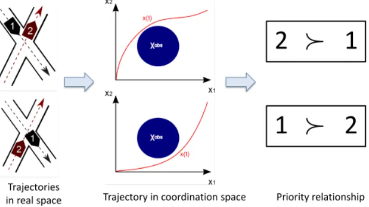
Fig. 1. An illustration of the concepts with 2 vehicles: real space, coordination space and priorities
We assume that vehicles move only forward so that the speed is always positive and bounded: ˙xi(t) ∈ [0, V ] for all
i and t. Note that for every couple of vehicles with a non-empty obstacle region, one vehicle necessarily passes before or after the other one, which naturally yields the notion of priorityas invariant of trajectories homotopy classes. We will not detail all aspects of this notion because it is not necessary for Theorem 1 but it is fundamental in the decision making we explain later. We assume a first-order control:
˙
x(t) = u(t, x(t)) (1) In a pure open-loop planning, the control u only depends on time: u = u(t), while in a pure feedback control, u depends
only on the state : u = u(x). We will study this second case. Note that a system subject to a first order feedback-controlled dynamics boils down to that case since we would have
˙
x = f (x, u(x)) = ˜u(x)
where ˜u : x → f (x, u(x)). Systems with higher order derivatives can also be considered but notation becomes bushy. The system starts at a point x0 where at least one
coordi-nate is zero (latest arrived vehicle). We must assume not only that all vehicles are not colliding (x06∈ χobs), but a stronger
hypothesis that x0 is not colliding and is reachable from 0 = (0, . . . , 0) 6∈ χobs by a continuous path of non-colliding
initial states. In other words the set of non-colliding initial states is connected. The end point is 1 = (1, . . . , 1). Note that when a vehicle reaches abscissa 1, it has no interaction with all other vehicles so that we can set its speed to V ; however, to keep the system within [0, 1]n, we halt it at 1 hence its speed
is null. This may lead to a discontinuity in the control but this is artificial and it can be technically handed out at the price of extra notation without benefit, so we will here set aside this technicality.
A trajectory {x(t), t ∈ [0, T ]} is feasible if x(0) is a starting point, x(T ) = 1 (liveness condition: there is a finite exit time), x(t) is collision-free for any t ∈ [0, T ] and
˙
x(t) ∈ [0, V ]n. For x0 to be eligible, we further assume that
x0does not necessary lead to a gridlock, therefore there exists a feasible trajectory with x(0) = x0. Our problem is to build
an efficient control as in Equation (1), mapping all eligible starting points into feasible trajectories (avoiding collisions and reaching the end point 1).
III. THEOREM
The main result of this paper is the following Theorem. Theorem 1: Consider a model of an intersection as de-scribed above. Then there is no feedback control u that is simultaneously smooth, that maps all eligible entry points into feasible trajectories and for which there are at least two distinct homotopy classes.
In order to sketch a rigorous proof, we need to further define our terms. Since we consider a feedback control u, the evolution of a state is given by
˙
x(t) = u(x(t)) and x(0) = x0. (2) This is a typical ordinary first-order differential equation whose properties are detailed in [17]. A classical smoothness condi-tion for u is to be Lipschitz continuous. Here we further know that u is bounded since 0 ≤ u ≤ V ; therefore trajectories exist, are unique and are defined for all t ≥ 0 (but we artificially stop the coordinates to keep trajectories within the compact set [0, 1]n). And the trajectories are continuous with respect
to their initial starting point (for any finite time horizon). To distinguish between starting points and trajectories, we shall denote by Φu(x0) a trajectory that is solution of the system (2),
i.e. Φu(x0, t) = x(t) for t ≥ 0. The choice a smooth feedback
control u yields a continuous mapping from the initial states into feasible trajectories: x0 → Φu(x0). Note that the set of
all Φu(x0) (for all feasible initial states) is a set of trajectories
and as such can be divided in homotopy classes that we call the homotopy classes of the control u (and to distinguish from
the priority graph and the homotopy classes of the feasible trajectories).
a) Proof: The proof shows the contradiction of the hypotheses. First we show that under the hypotheses, there exists a uniform bound for exit times. By hypothesis, for each starting point x0, there exists an exit time denoted by T (x0).
Assume infx0T (x0) = ∞. Then there exists a sequence of
starting points with indefinitely increasing exit times. Since the set of entry points is compact (the obstacle region χobs
is open and so are the invalid starting points), there exists a point of accumulation for this sequence. By continuity of the trajectories, the exit time for the trajectory associated with that entry point is infinite. This contradicts the existence of an exit time (liveness condition). Therefore infx0T (x0) = T < ∞.
Since the exit time is uniformly bounded, all trajectories are globally continuous with respect to their starting points. Now, we assumed that all starting points are reachable from starting point 0. This means we can build a continuous path of starting points from any pair of starting points. By continuity of the trajectories with respect to their starting points, this means there exists a continuous transformation between any pair of feasible trajectories: hence there exists a unique homotopy class. This contradicts the hypothesis of having at least two homotopy classes.
The proof is concluded with this contradiction.
The author is aware of a few hidden technicalities. Just to mention one, the proof that the entry set is compact is made difficult because we excluded the initial states that lead necessarily to a gridlock. This is very technical. If one can (by making too simple assumptions) exclude the accumulation points of the above proof, then we in fact cut the entry set into disconnected components and there is a smooth control on each one: this means we can have several homotopy classes for this control with their own smooth feedback control. But this is artificial in the sense that we exclude exactly the critical points for which the control leads to a deadlock.
IV. THEORETICAL AND PRACTICAL CONSEQUENCES
This section intends to make Theorem 1 and its conse-quences clearer. We begin by a review of our main assump-tions. Then formulate some theoretical corollaries and provide an analysis of the meaning of Theorem 1 in term of decision. Finally we discuss what can be the practical implication of Theorem 1: can we use it to improve state-of-the art systems? A. Discussion of hypotheses
Several assumptions have been made. We will not discuss some well established hypotheses because it has been made previously: the coordination space and its fixed path assump-tion is considered as relevant.
The first hypothesis we made is the smoothness of the control: it should be Lipschitz continuous. This is not an obvious assumption and we will exhibit later some non-smooth (discontinuous) control that could fit with a better cooperative control. However most of the controls, especially distributed controls (swarms...) are smooth (and even several times differ-entiable). This is because feedback control is related to errors
and uncertainties: a discontinuous control may easily lead to unstable systems (and practically to vibrations). Due to errors in the perception, the measured state would jump from one side of the discontinuity to the other side leading to sudden changes in the control. To our knowledge, there is few work on discontinuous feedback control.
Fig. 2. Illustration of a blocking initial point: The blue disk is the obstacle region; the white region is collision-free and there the feedback control is represented as a vector field (black arrows); the trajectories are the integral lines (e.g. green line for the vectors represented). The black integral line starting from the lower-left corner (point 0) never ends because when approaching the obstacle region the vector field vanishes: it is a critical trajectory. It splits the trajectories in 2 homotopy classes (red and green) with 2 different priorities.
The second strong hypothesis concerns the critical trajec-tories, mentioned at the end of the previous section as the the trajectories corresponding to accumulation (initial) points in the proof. Besides the technicalities that were detailed, we can explain the existence of these critical trajectories. There are indeed lots of them because they mark the boundary between two homotopy classes. Let us consider the case with n = 2 and an X crossing with one vehicle from south and the second from east; each go straight. When vehicles arrive at very different times, there is no interaction so they can drive normally (say at maximum speed). When they arrive at the same time, rules (say priority to the right) apply and south vehicle has to let east vehicle pass. But how long has south to wait? Now Theorem 1 states that there exists a time when east vehicle arrives later than the south vehicle and there is a conflict between south having to wait and willing to pass: if this priority rule is softly encoded (by a continuous control), it leads to a deadlock; an illustration of this is also given in Figure 2. So one way to do is to exclude these critical trajectories (or have a special processing), but it would be rather artificial since a slightly different control would move this boundary. We show later it should be better considered as a question of decision, not of control. Please note that the word priority in this paragraph
is related to the rules while in the priority framework the same word is related to a topological invariant: the semantics is related but not exactly the same.
The third hypothesis is related to the uniqueness of the homotopy class. In a normal cooperative system there are many homotopy classes (encoded by a priority graph, or priority for short). As soon as two vehicles may collide, there is a non-empty collision set, leading to two classes of trajectories: one vehicle first or second. We have shown in the previous paragraph what are the consequences of this division. Thereafter we will always assume we have a system with several (indeed huge) number of priority graphs (the number of binary relations between n objects). Note that there are two ways to define homotopy classes: in the space of feasible trajectories and the subset of trajectories generated by a control u which is one-to-one with the entry points. Theorem 1 can be seen as stating that choosing a smooth control u forces to chose only one priority among all possibilities.
B. Theoretical consequences
The previous section shows that under rather acceptable assumptions there are interesting consequences of Theorem 1. This section intends to show that Theorem 1 explicits the idea of decision. A decision is seen here as a discrete choice that impacts the control the system. The last paragraph of the previous section gives a hint toward that: adopting a smooth feedback control u means an implicit decision making: a unique priority is encoded into u. It is very clear (and our previous papers explicit this construction) that it is better to first decide which priority is best, then to build a smooth feedback control. This is explicit versus implicit decision making. And we see that the decision is related to priorities: it is precisely the choice of one priority graph, i.e. one homotopy class. Note that Theorem 1 does not give any hint about the choice of the best priority, but it tells we have to make a choice. Not making a choice leaves it implicit or potentially inefficient as the next corollary states.
Corollary 1: For a system as in Theorem 1, for any smooth feedback control u mapping entry points into at least two distinct homotopy classes, there exists an entry point for which the system will globally stop (gridlock).
This is a consequence of the Theorem: we have assumed existence and continuity of u, but several realized homotopy classes (meaning trajectories produced by u are not all homo-topic). Therefore the last assumption is not true: some initial points have non-feasible trajectories.
From previous discussion we see that these critical trajecto-ries are at the boundary between two homotopy classes. Note that the system globally stops but some vehicles may have passed the intersection. We simply mean that the exit time is infinite (indeed the remaining vehicles will not be stopped but their speed will decrease exponentially) so that a subset of vehicles remains blocked within the intersection.
A partial solution to that challenge would be to consider discontinuous controls. Indeed, in our previous crossing exam-ple, we can set a time where south is first and goes maximal speed, then east is first and goes maximal speed (and assume this holds also for the exact time). This control is clearly dis-continuous but makes somehow sense. Of course there should
be no error otherwise both vehicles could collide at maximum speed. In fact a deeper analysis shows that the critical trajectory is highly unstable so that the system can reach quickly safe trajectories. But this requires a discontinuous control with an arbitrary critical point.
The previous consideration reveals the need for an ef-ficiency criteria. Unfortunately such a criteria is difficult: a fairly good one is the total exit time defined above. However it is not always very helpful. Another criteria is to have a work-conservative system: at least one vehicle should be at maximum speed in the intersection. It is weaker than the total exit time but easier to use. A smooth control can be work-conservative but only within one priority: this means that some vehicles can wait a lot without any need. So we would like to define work-conservative as maintaining at least one vehicle at maximum speed within the colliding area (a much more limited area). Unfortunately such an area is difficult to formalize. But keeping the idea, one sees that the vehicle that goes maximum speed cannot be determined by a continuous control: this is the decision to take.
This is how we envision future work: when vehicles are rather far from each other, a smooth control is used. When they arrive in areas where collision may happen, a decision has to be taken. This decision has to be taken for at least the two of them, most probably using communication. Once the decision is taken the vehicles can again follow a smooth control. Such a method also show that priorities must be decided in a timely manner: allocating priorities too early is not optimal.
C. Practical consequences
As we have seen previously in our discontinuous control example, critical trajectories are generally unstable. This ex-plains why practically smooth feedback control is so effective and useful. Theorem 1 shows here only two things: first in very complex situation this instability could be slow and it could be worth having more “aggressive” schemes like discontinuous control. Second, some kind of discrete decision making could enhance the reactive schemes (using any kind of signals).
Finally we conclude with a very obvious remark from the daily life: a big question is where and when to take decision. This refers mathematically to ambiguous (or critical) starting points: these are the place where there is a need for cooperative decision. Now we believe the decision has to be taken in a neighborhood of these critical points. And the precise place where decision should be taken is almost surely related to the noise model. It is obvious that with neither noise nor error an open loop scheme is optimal so that we can have an early decision, even an implicit decision making. This is surely not true for stochastic models.
V. CONCLUSION
This paper highlights a negative theorem linking feedback control, choice and efficiency. This theorem shows that we can-not expect building optimal controls for cooperative systems with a purely reactive scheme. Some decision are to be taken. And we highlight the need for a well designed decision making in order to keep a system reactive with feedback control.
This paper is intentionally made simple to start the dis-cussion during the ITSC conference, before a more detailed paper in a journal with a more rigorous proof. For the same reason I allow myself to raise an interesting point made by a reviewer was: “Is reactive scheme (feedback control) the only choice? A lot of optimal control strategies, like MPC, also only require local information”. My belief is that as soon as MPC criteria are smooth and local (and for any control strategy), an equivalent of Theorem 1 holds. This is clearly more difficult to prove (especially the local part of it) though the same concepts hold.
Future research has been stated in several places of this paper. There is a large avenue of research for cooperative control: optimizing the place where decision have to be taken, trying to have a distributed decision making using suitable communication protocols, designing good feedback controls that fit well with the decision making (e.g. avoiding a discon-tinuity at the time of the decision)...
REFERENCES
[1] J. van Dijke, M. van Schijndel, F. Nashashibi, and A. de La Fortelle, “Certification of automated transport systems,” Procedia-Social and Behavioral Sciences, vol. 48, pp. 3461–3470, 2012, presented at TRA 2012 and selected as a paper: special issue for Transport Research Arena 2012. [Online]. Available: http://www.sciencedirect.com/science/article/pii/S1877042812030534 [2] A. de La Fortelle, X. Qian, S. Diemer, F. Moutarde, and S. Bonnabel,
“Network of automated vehicles: the autonet2030 vision,” in ITS World Congress, 2014.
[3] T. Fraichard and H. Asama, “Inevitable collision states - a step towards safer robots?” Advanced Robotics, vol. 18, pp. 1001–1024, 2004. [4] R. R. Negenborn, B. De Schutter, and J. Hellendoorn, “Multi-agent
model predictive control for transportation networks: Serial versus parallel schemes,” Engineering Applications of Artificial Intelligence, vol. 21, no. 3, pp. 353–366, 2008.
[5] M. Papageorgiou, C. Diakaki, V. Dinopoulou, A. Kotsialos, and Y. Wang, “Review of road traffic control strategies,” Proceedings of the IEEE, vol. 91, no. 12, pp. 2043–2067, 2003.
[6] L. Makarem and D. Gillet, “Model predictive coordination of au-tonomous vehicles crossing intersections,” in Intelligent Transportation Systems - (ITSC), 2013 16th International IEEE Conference on, Oct 2013, pp. 1799–1804.
[7] J. Gregoire, X. Qian, E. Frazzoli, A. de La Fortelle, and T. Wongpirom-sarn, “Capacity-aware back-pressure traffic signal control,” Proceedings of IEEE TCNS, 2014.
[8] L. Makarem, M. H. Pham, A.-G. Dumont, and D. Gillet, “Micro-simulation Modeling of Coordination of Automated Guided Vehicles at Intersection,” in Transportation research board 91st annual meeting, 2012.
[9] K. Kant and S. Zucker, “Planning collision-free trajectories in time-varying environments: a two-level hierarchy,” The Visual Computer, vol. 3, no. 5, pp. 304–313, 1988. [Online]. Available: http://dx.doi.org/10.1007/BF01914866
[10] K. Dresner and P. Stone, “Multiagent traffic management: A reservation-based intersection control mechanism,” in The Third International Joint Conference on Autonomous Agents and Multiagent Systems, July 2004, pp. 530–537. [Online]. Available: http://www.cs.utexas.edu/users/ai-lab/?AAMAS04
[11] S. M. LaValle, Planning Algorithms. Cambridge, U.K.: Cambridge University Press, 2006, available at http://planning.cs.uiuc.edu/. [12] A. de La Fortelle, “Analysis of reservation algorithms for cooperative
planning at intersections,” in Intelligent Transportation Systems (ITSC), 2010 13th International IEEE Conference on, Sept 2010, pp. 445–449. [13] A. Charalampidis and D. Gillet, “Speed profile optimization for ve-hicles crossing an intersection under a safety constraint,” in Control Conference (ECC), 2014 European, June 2014, pp. 2894–2901.
[14] J. Gregoire, S. Bonnabel, and A. de La Fortelle, “Priority-based coordination of robots,” CoRR, vol. abs/1306.0785, 2013. [Online]. Available: http://arxiv.org/abs/1306.0785
[15] ——, “Priority-based intersection management with kinodynamic con-straints,” in Control Conference (ECC), 2014 European, June 2014, pp. 2902–2907.
[16] X. Qian, J. Gregoire, F. Moutarde, and A. D. L. Fortelle, “Priority-based coordination of autonomous and legacy vehicles at intersection,” in Intelligent Transportation Systems - (ITSC), 2014 17th International IEEE Conference on, Oct 2014.
[17] P. Hartman, Ordinary Differential Equations, 2nd ed. Society for Industrial & Applied Math, 2002, iSBN 0-89871-510-5.