Face recognition based on composite correlation filters: analysis of their performances

HAL Id: hal-00782961

https://hal.archives-ouvertes.fr/hal-00782961

Submitted on 31 Jan 2013

HAL is a multi-disciplinary open access

archive for the deposit and dissemination of

sci-entific research documents, whether they are

pub-lished or not. The documents may come from

teaching and research institutions in France or

abroad, or from public or private research centers.

L’archive ouverte pluridisciplinaire HAL, est

destinée au dépôt et à la diffusion de documents

scientifiques de niveau recherche, publiés ou non,

émanant des établissements d’enseignement et de

recherche français ou étrangers, des laboratoires

publics ou privés.

Face recognition based on composite correlation filters:

analysis of their performances

Isabelle Leonard, Ayman Alfalou, Christian Brosseau

To cite this version:

Isabelle Leonard, Ayman Alfalou, Christian Brosseau. Face recognition based on composite correlation

filters: analysis of their performances. Face Recognition: Methods, Applications and Technology, A.

Quaglia and C. M. Epifano, pp.57-80, 2012. �hal-00782961�

Face recognition based on composite correlation

filters: analysis of their performances

I. Leonard1, A. Alfalou,1 and C. Brosseau2 1 _{ISEN Brest, Département Optoélectronique, L@bISEN,}

20 rue Cuirassé Bretagne, CS 42807, 29228 Brest Cedex 2, France E-mail: ayman.al-falou@isen.fr

2 _{Université Européenne de Bretagne, Université de Brest, Lab-STICC,}

CS 93837, 6 avenue Le Gorgeu, 29238 Brest Cedex 3, France E-mail: brosseau@univ-brest.fr

Abstract

This chapter complements our paper: ”Spectral optimized asymmetric segmented phase-only correlation filter ASPOF filter” published in Applied Optics (2012).

1. Introduction

Intense interest in optical correlation techniques over a prolonged period has focused substantially on the filter designs for optical correlators and, in particular, on their important role in imaging systems using coherent light because of their unique and quite specific features. These techniques represent a powerful tool for target tracking and identification [1].

In particular, the field of face recognition has matured and enabled various technologically important applications including classification, access control, biometrics, and security systems. However, with security (e.g. fight terrorism) and privacy (e.g. home access) requirements, there is a need to improve on existing techniques in order to fully satisfy these requirements. In parallel with experimental progress, the theory and simulation of face recognition techniques has advanced greatly, allowing, for example, for modeling of the attendant variability in imaging parameters such as sensor noise, viewing distance, emotion recognition facial expressions, head tilt, scale and rotation of the face in the image plane, and illumination. An ideal real-time recognition system should handle all these problems.

It is within this perspective that we undertake this study. On one hand, we make use of a Vander Lugt correlator (VLC) [2]. On the other hand, we try to optimize correlation filters by considering two points. Firstly, the training base which serves to qualify these filters should contain a large number of reference images from different viewpoints. Secondly, it should correspond to the requirement for real-time functionality. For that specific purpose, our tests are based on composite filters. The objectives of this chapter are first to give a basic description of the performances of standard composite filters for binary and grayscale images and introduce newly designed ASPOF (asymmetric segmented phase-only filter), and second to examine robustness to noise (especially background noise). This paper deals with the effect of rotation and background noise problems on the correlation filtering performance. We shall not treat the deeper problem of lighting problems. Phong [3] described methods that are useful to overcome the lighting issue in terms of laboratory observables.

Adapted playgrounds for testing our numerical schemes are binary and grayscale image databases. Each binary image has black background with a white object (letter) on it with dimension 512 x 512 pixels. Without loss of generality, our first tests are based on the capital letters A and V because it is easy to rotate them with a given rotation angle (procedures for other letters are similar). Next simulations were performed to illustrate how this algorithm can identify a face with grayscale images from the Pointing Head Pose Image Database (PHPID) [4] which is often used to test face recognition algorithms. In this study, we present comprehensive simulation tests using images of five individuals with 39 different images captured for each individual.

We pay special attention to adapting ROC curves for different phase only filters (POFs), for two reasons. Firstly, POFs based correlators and their implementations have been largely studied in the literature, see e.g. [1, 5]. In addition, optoelectronics devices, i.e. spatial light modulators (SLMs) allow implementing optically POFs in a simple manner. Secondly, numerical implementation of correlation have been considered as an alternative to all-optical methods because they show a good compromise between their performance and their simplicity. High speed and low power numerical processors, e.g. field programmable gate array (FPGA) [6] provide a viable solution to the problem of optical implementation of POFs. Such numerical procedure allows one to reduce the

memory size (by decreasing the number of reference images included in the composite filter) and does not consider the amplitude information which can be rapidly varying. Face identification and underwater mine detection with background noise are two areas for which the FPGA has demonstrated significant performance improvement, such as image registration and feature tracking. Following this brief introduction, we have divided the rest of the paper as follows: a general overview of the optical correlation methods is given in Sec. 2. Then, in Sec. 3, we review a series of correlation filters, which are next compared in Sec. 4

2. Some preliminary considerations and relation to previous work

The subject of correlation methods is long and quite a story. Here we will review various aspects of the problem discussed in the literature which relate to this paper. The modern study of optical correlation can be traced back to the pioneering research in the 1960s [2, 7]. In what became a classic paper, Vander Lugt presented a description of the coherent matched filter system, i.e. the VLC [2]. Basically, this method is based on the comparison between a target image and a reference image. This technique consists in multiplying an input signal (spectrum of image to be recognized) by a correlation filter, originating from a training base (i.e. reference base), in the Fourier domain. The result is a correlation peak (located at the center of the output plane i.e. correlation plane) more or less intense, depending on the degree of similarity between the target image and reference image. Correlation is perceived like a filtering which aims to extract the relevant information in order to recognize a pattern in a complex scene. However, this approach requires considerable correlation data and is difficult to realize in real time. This led to the concept of POF (carried out from a single reference) whose purpose is to decide if a particular object is present or not, in the scene. To have a reliable decision about the presence, or not, of an object in a given scene, we must correlate the latter with several correlation filters taking into account the possible modifications of the target object, e.g. in-plane rotation and scale. Perhaps more problematic is the fact that a simple decision based on the presence, or not, of a correlation peak is insufficient. Thus, use of adequate performance criteria such as those developed in [8-9] is necessary.

During the 1970s and 1980s correlation techniques developed at a rapid pace. A plethora of advanced composite filters [10-12], and more general multi-correlation approaches [13] have been introduced. A good source for such results is the book of Yu [14]. However, experimental state of the art shows that optical correlation techniques almost found themselves in oblivion in the late 1990s for many reasons. While numerous schemes for realizing all-optical correlation methods have been proposed [13-15], up to now, they all face technical challenge to implement, notably those using spatial light modulators (SLMs) [16] because these methods are very sensitive to even small changes in the reference image. In addition, they usually require a lot of correlation data and are difficult to realize in real time.

Over the last decade, there has been a resurgence of interest, driven by recognition and identification applications [17-22], of the correlation methods. For example, Alam et al. [22] demonstrated the good performances of the correlation method compared to all numerical ones based on the independent component model. Another significant example in this area of research is the work by Romdhani et al. [23], which compared face recognition algorithms with respect to those based on correlation. Other recent efforts include the review by Sinha et al. [24] dealing with the current understanding regarding how humans recognize faces. Riedel et al. [25] have used the minimum average correlation energy (MACE) and unconstrained MACE filters in conjunction with two correlation plane performance measures to determine the effectiveness of correlation filtering in relation to facial recognition login access control. Wavelets provide another efficient biometric approach for

facial recognition with correlation filters [26]. A photorefractive Wiener-like correlation filter was also

introduced by Khoury et al. [27] to increase the performance and robustness of the technique of correlation filtering. Their correlation results showed that for high levels of noise this filter has a peak-to-noise ratio that is larger than that of the POF while still preserving a correlation peak that is almost as high as that of the POF.

Another optimization approach in the design of correlation filters was addressed to deal with the ability to

suppress clutter and noise, an easy detection of the correlation peak, and distortion tolerance [28]. The resulting maximum average correlation height (MACH) filter exhibit superior distortion tolerance while retaining the attractive features of their predecessors such as the minimum average correlation energy filter and the minimum variance synthetic discriminant function filter. A variant of the MACH filter was also developed in [29]. Pe‟er and co-workers [30] presented a new apochromatic correlator, in which the scaling error has three zero crossings, thus leading to significant improvement in performance. These references are far from a complete list of important advances, but fortunately the interested reader can easily trace the historical evolution of these ideas

with Vijaya Kumar„s review paper, Yu‟s book, and the chapter of Alfalou and Brosseaucontaining an extensive

bibliography [1, 14-15, 31]. As mentioned above, we have a dual goal which is first to introduce standard correlation filters, and second to compare their performances.

3. A brief overview of correlation filters

First we present the most common correlation filters. We turn attention to the general merits and drawbacks of composite filters. This discussion is simply a brief review and tabulation of the technical details for the basic composite filters. For that purpose we consider a scene s containing a single or several objects o with noise b.

The input scene is written as s x y



,



o x y



,



b x y



,



. Let its two-dimensional FT be denoted by



,





,



exp



,



S      _i   _. In the Fourier plane of the optical set-up, the scene spectrum is multiplied by

a filter H



 ,



, where  and  denote the spatial frequencies coordinates. Many approaches for designing

filters to be used with optical correlators can be found in the literature according to the specific objects that need to be recognized. Some have been proposed to address hardware limitations; others were suggested to optimize a merit function. Attempts will be made throughout to use a consistent notation.

3.1. Adapted filter (Ad)

The Ad filter [2] has for main purpose to optimize the SNR and reads

      * , , , A d b R H          (1)

where  denotes a constant, *





,

R   is the complex conjugate of the spectrum of the reference image

(R



 ,



   ₀



,



exp



i  ₀



,





), and _b



 ,



represents the spectral density of the input noise. If we

assume that the noise is white and unit spectral density, we obtain H_Ad



,



R*



,



. A main advantage

of this filter is the increase of the SNR especially when white noise is present. The drawback of this filter is that it leads to broad correlation peaks in the correlation plane. Since the output plane is scanned for this peak, and its location indicates the position of the target in the input scene, we can conclude that the target is poorly localized.

In addition, its discriminating ability is weak.

3.2. Phase-only filter (POF)

The phase is of paramount importance for optical processing with coherent light [32]. For example, Horner and Gianino [33] suggested a correlation filter which depends only on the phase of a reference image (with which the scene is compared). Without loss of generality, this POF is readily expressible as

     



 



* 0 , , exp , , P O F R H i R             (2)

The main feature of the POF is to increase the optical efficiency . It is worthy to note that Eq. (2) depends

only the phase of the reference. Besides the ability to get very narrow correlation peaks, POF have another feature that Ad filters lack: the capacity for discriminating objects. Because POF use only the reference‟s phase,

they can be useful as edge detector. However, as is well known the POF isvery sensitive to even small changes

in rotation, scale and noise contained in the target image [34].

3.3. Binary phase-only filter (BPOF)

We consider next the binarized version of the phase-only filter [35], or alternatively defined as a two-phase filter where the only allowed values are 1 and -1 such as

1 B P O F

H  if the real part of POF filter 0

1 B P O F

H   _otherwise

(3)

Other definitions of BPOF were also considered by Vijaya Kumar [36]. Generally, BPOF have weaker performances than POF. It is helpful in certain applications for which the size of the filter should be small and

also for optical implementation. Like POF, BPOF is very sensitive to rotation, scale, and noise in the target images.

3.4. Inverse filter (IF)

IF [37-38] is defined as the ratio of POF by the magnitude of the reference image spectrum, and can be expressed as        





  * 0 2 0 ex p , , , , , IF i R H R                (4)

The main advantage of this filter is to minimize the correlation peak width, or in other words, to maximize the PCE. It has the desirable property of being very discriminating. Despite this, an IF has a number of

drawbacks. It is very sensitive to deformation and noise contained in the target image with respect to the

reference image.

3.5. Compromise optimal filter (OT)

To realize a good correlation, the filter should be discriminating and robust. A filter showing a trade-off between these two properties was suggested in [39]. The OT filter is conveniently written out as

              * 0 0 2 2 2 0 , ex p , 1 , 1 , O T b b R i H R                         (5)

where α denotes a discrimination and robustness degree. If  is set to zero, Eq. (5) yields the inverse filter,

while the adapted filter is recovered when α is equal to one.

3.6. Classical composite filter (COMP)

In general, taking a decision based on a single correlation obtained by comparing the target image with only one filter, i.e. single reference, does not allow getting a reliable identification [31]. To alleviate the problems associated with this drawback, correlation approaches have been suggested. One way to realize multi-correlation within the VLC configuration is by employed the classical composite filter (COMP). The basic idea consists in merging several references by linearly combining them such as

    1 , , M C om p i i H   R    



(6)

where R_i



 ,



denotes each reference spectrum. Observe that a weighing factor can be used in some cases

for specific purpose [13].

3.7. Segmented composite filter (SPOF)

For the purpose of reducing the number of correlation requested to take a reliable decision, the number of

references in the filter should be increased. However, increasing the latter has for effect to induce a local

saturation phenomenon in a classical composite filter [5]. This can be remedied by use of a recently proposed spectral multiplexing method [5]. This method consists in suppressing the high saturation regions of the reference images. Briefly stated, this is achieved through two steps [5]. First, a segmentation of the spectral plane of the correlation filter is realized into several independent regions. Second, each region is assigned to a single reference. This assignment is done according a specific energy criterion

, , , , , , l k u v u v l k i j i j i j i j E E E E  





(7)

This criterion compares the energy (normalized by the total energy of the spectrum) for each frequency of a

given reference with the corresponding energies of another reference.Assignment of a region to one of the two

references is done according Eq. (7). Hence, the SPOF contains frequencies with the largest energy.

3.8. Minimum average correlation energy (MACE)

For good location accuracy in the correlation plane and discrimination, we need to design filters capable of producing sharp correlation peaks. One method [12] to realize such filters is to minimize the average correlation plane energy that results from the training images, while constraining the value at the correlation origin to certain prespecified values. This leads to the MACE filter which can be expressed in the following compact form:



 



 



D S S D S c

H_MACE 1 1 1 (8)

where D is a diagonal matrix of size d d, (d is the number of pixels in the image) containing the average

correlation energies of the training images across its diagonals; S is a matrix of size Nd where N is the number

of training images and + is the notation for complex conjugate. The columns of the matrix S represent the Discrete Fourier coefficients for a particular training image. The column vector c of size N contains the correlation peak constraint values for a series of training images. These values are normally set to 1 for images of the same class [14]. A MACE filter produces outputs that exhibit sharp correlation peaks and ease the peak detection process. However, there is no noise tolerance built into these filters. In addition, it appears that these

filters are more sensitive to intraclass variations than other composite filters [40].

3.9. Amplitude-modulated phase-only filter (AMPOF)

Awwal et al. [21, 28] suggested an optimization of the POF filter based on the following idea: if the

correlation plane of the POF spreads large, it yields a correlation peak described by a Dirac function. One way to

realize this has been put forward in Ref. [21, 28], where the authors suggested the amplitude-modulated phase-only filter (HAMPOF)

















ex p , , , A M P O F D j H F a           (9)

where F



 ,



 F



 ,



exp



j  



,





is the reference image spectrum,  and  denote the spatial frequencies, D is a parameter within the range ]0,1], and the factor a (aD) appearing in the denominator is

useful in overcoming the indeterminate condition and ensuring that the gain is less than unity. It can be a

constant or a function of µ and ν, and thus can be used to either suppress noise or bandlimit the filter or both.

3.10. Optimal trade-off MACH (OT MACH)

Another optimization approach in the design of correlation filters was addressed to deal with the ability to

suppress clutter and noise, an easy detection of the correlation peak, and distortion tolerance [28]. The resulting maximum average correlation height (MACH) filter exhibit superior distortion tolerance while retaining the attractive features of their predecessors such as the minimum average correlation energy filter and the minimum variance synthetic discriminant function filter. A variant of the MACH filter was also developed in [29], i.e. the optimal trade-off MACH filter which can be written as

* x O T M A C H x x m H C D S       (10)

where mx is the average of the training image vectors, C is the diagonal power spectral density matrix of the

additive input noise, Dx is the diagonal average power spectral density of the training images, Sx denotes the

3.11. Asymmetric segmented phase only filter (ASPOF)

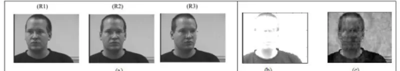
The last filter which is presented in this chapter is the ASPOF. See, e.g. [41], for its definition. The reference image database is divided in two sub-databases (with reference to Fig.1).

Fig 1: Technique used to separate the reference images into 2 sub-classes [41] A SPOF is constructed from each of these databases according to the criterion defined by Eq.11.

(11)

Pixels which are not assigned using Eq.(11) are further assigned to the majority reference in the pixel's neighborhood (see Fig.2).

? ? ? ? ? ? ? ? ? S = Spectre l S = Spectre l k k (a) (b) (c) (d)

Isolated pixel not affected: Before procedure

Isolated pixel affected: After procedure

Fig 2: Illustrating the optimized assignment procedure for isolated pixels [41].

4. Comparative study of composite correlations filters with binary images

Much research has been devoted to discovering new composite filters with higher efficiencies. An extensive review of composite filters has been found to be given by, where much can be found about distortion-invariant optical pattern recognition. In particular, there are many other facets of composite filters not mentioned in section (3). In a general context, it is instructive to compare the performance of a selection of composite filters described in section (3). To aid the reader of this section, we briefly recap the filters characteristics and some of our terminology in Table 1. The main goal of this section is to identify the parameters which introduce limitations in the performances of these composites filters with and without noise in the input plane.

The binary (black and white) images from Fig. 3 (a)-(c) were chosen for testing the composite filters because they are easier to process and analyze than gray level images, and the letter base can be digitized under controlled conditions, i.e. easy to process morphological operation and addition of input noise. Each image has

black background with a white object (letter) on it with dimension 512512 pixels. Here, we will limit ourselves

Fig 3: (Color online) Binary image for the uppercase letter A in the English alphabet: (a) standard, (b) 90° counterclockwise rotation, (c) the same as a 90° clockwise rotation, (d) PCEs obtained with the composite adapted filter. The colors shown in the inset denote the different composite adapted filters depending on the

number of references used

We now compare in a systematic way the performances of the composite filters of Table I for the data-base displayed in Fig. 1(a)-(c). In performing this comparison a normalization of the correlation planes was realized. An illustration of the effects of the number of reference images (typically ranging from 1 to 37) employed to realize the composite filter on rotation of the input image will also be given.

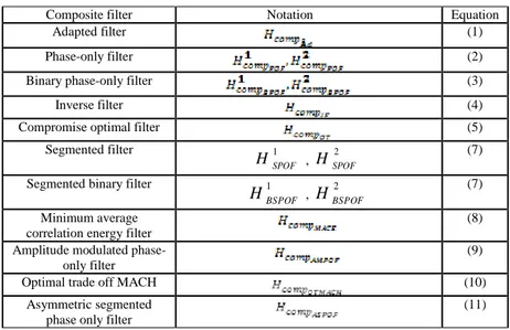
Table 1: illustrating the different composite filters used.

Ad

comp

H denotes the Adapted composite filter. This later is realized by considering a linear combination of reference images, and then using the adapted filter definition (Eq. (1)). HComp-POF is the POF

composite filter. We tested two different schemes for realizing the Composite POF filter. In the first scheme ( 1

POF comp

H ) we used a

linear combination of reference images to create the POF, i.e. Eq. (2). The second scheme ( 2

POF comp

H ) involves performing the

POF, via Eq. (2), for each reference, and then using the linear combination of these POFs. 1

BPOF comp H and 2 BPOF comp H are the

binarized versions of the filters 1

POF comp

H and 2

POF comp

H obtained from Eq. (3), respectively. The composite inverse filter

IF

comp

H is the inverse filter (Eq. (4)) of the linear combination of reference images. The optimal composite filter

OT

comp

H is

realized by linearly combining reference images (Eq. (5)). 1

SPOF comp

H denotes the segmented filter realized by doing segmentation and assignment with the energy criterion (Eq. (7)). The calculation of filter 2

SPOF comp

H is done by replacing the energy in Eq. (7) with the square of the real part of the different references spectra to be merged.

MACE comp

H is the composite filter of the MACE

filter developed in Eq. (8).

AMPOF

comp

H is the composite version of AMPOF (Eq. (9)). is the composite version of

OTMACH (Eq.(10)). is the ASPOF (Eq.(11)). [41]

Composite filter Notation Equation

Adapted filter (1)

Phase-only filter (2)

Binary phase-only filter (3)

Inverse filter (4)

Compromise optimal filter (5)

Segmented filter 1

SPOF

H , H_SPOF2 (7)

Segmented binary filter 1

BSPOF

H , H_BSPOF2 (7)

Minimum average correlation energy filter

(8)

Amplitude modulated phase-only filter

(9)

Optimal trade off MACH (10)

Asymmetric segmented phase only filter

4.1. Adapted composite filter

We start our discussion by considering the adapted composite filter in the Fourier plane of the VLC. Fig. 3 (d) shows PCE by introducing every image of the data-base of 181 images, one by one, in the entrance plane. Each curve of Fig. 1 (d) has a specific color which depends on the number of references used to realize the adapted filter, e.g. the red one considers a 3-reference filter (-5°, 0°, and 5°). As expected the adapted composite filter is robust against rotation. It is also worthy to observe that the energy contained in the correlation peak decreases as the number of references chosen to realize the filter is raised. This decrease is detrimental to the usefulness of this type of composite filter. Its low discriminating character is more and more visible as the number of references is increased. This is consistent with previous studies [13].

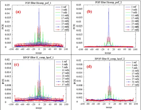
4.2. Composite POF

Fig. 4 (a) shows the PCE results for the composite POF 1

POF comp H . As described previously, 1 POF comp H is

realized by considering a linear combination of reference images (ranging from 1 to 37) to create a composite image. The input images are then correlated with this filter. We find that the energy contained in the correlation peak decreases significantly, i.e. the PCE is decreased by a factor of 3 when using a POF containing 3 references by contrast with a POF realized with a single reference. For a 11-reference POF, the PCE is decreased by an order of magnitude which renders unreliable the decision on the letter identification. For 3 references only the images forming the filter are recognized. However, beyond 11 references, the weakness of the magnitude of the PCE makes the recognition of the images forming the filter very difficult.

Fig 4: (Color online) (a) PCEs obtained with the POF composite filter. The colors shown in the inset denote the different filters depending on the number of references used. (b) Same as in (a) for filter Hcomp_pof_2 . (c) and

(d) Same as in (a) and (b) for Binary filter

Fig. 4 (b) shows the correlation obtained with filter 2

POF comp

H which is obtained by linearly combining the

different POFs of different reference images. The magnitude of the PCE decreases with raising the number of reference images of the filter. From the point of view of recognition application it appears that the saturation

problem is more serious than that obtained with filter 1

POF comp

H , i.e. it is difficult to recognize a letter with a filter composed of more than 5 reference images even if the letter to be recognized belongs to the set of reference images. Thus, the overall performance for letter identification using this correlation technique decrease by

employing filter 2

POF comp

H .

From the combined observations above, an especially meaningful feature emerges: to get a reliable decision, a 3-reference POF should be used. One of the distinctive features shown in Fig. 4 (a) is that this filter allows one

to recognize the letter A only taking a range for angle of rotation from -7° to 7°. Recognition of the full base requires fabricating at least 12 POFs, each having 3 references. Hence, this procedure cannot permit significant reduction in the time of decision since other phenomena can also affect the target image, e.g. scale.

4.3. Composite binary POF

Binarized POF in the Fourier domain (Eq. (3) ) is an alternative to POF. Fig. 4 (c) (resp. Fig. 4 (d)) shows

PCE results obtained by binarization of 1

POF comp

H (resp. 2

POF comp

H ). Our calculations shown in these two graphs

can be discussed in the same way as was done for Figs. 2 (a) and (b). At the same time, a comparison between Figs. 4 (a) and (b) and Figs. 4 (c) and (d) indicates a decrease of the PCE values. This is reminiscent of the noise induced by the binarization protocol.

4.4. Inverse composite filter

It has been known for a while that the inverse filter shows a strong discriminating ability and a low robustness against small changes of the target image with respect to the reference image. In practice,

IF

comp

H is

realized by defining the inverse filter of the linear combination of different references. In Fig. 5 we plot the corresponding PCE values for the letter base A correlated with filter

IF

comp

H and different numbers of

references. These results are consistent with our previous observation of the PCE decrease as the number of references is raised. We also check that these simulations are consistent with the above mentioned characteristics of the inverse filter. Indeed, correlation vanishes even when the target image is identical to one of the reference images used to realize the filter.

Fig 5: (Color online) PCEs obtained with the inverse composite filter. The colors shown in the inset denote the different adapted filters depending on the number of references used [41].

Up to now, our results show that filter 1

POF

comp

H has the best performance among the selected composite filters

studied so far. To orient the subsequent discussion, we show the good discriminating ability of the composite POF, with parameters chosen for comparison with the above-described data. Our previous calculations suggest that the more discriminating efficiency of the filter is associated with the weaker false alarm rate. For that specific purpose, the letter V base (Fig.6 (a)), i.e. constituted by 19 images obtained by rotating the V every 10°,

was correlated with filter 1

POF

comp

H realized with reference images of letter A. Although the letter V has a great

similarity with the letter A with a 180° rotation, it is easily seen that the different composite POFs do not recognize V as being an A since no false alarm can be detected (Fig.6 (b)). Nominal values of PCE are less than 0.002, ca. over 20 times less than the maximum value seen in Fig. 4 (c). This is a clear indication of the good discriminating ability of the POF.

Fig 6: (Color online) Discrimination tests: (a) The target image considered is the letter V. (b) PCEs obtained with a filter realized with reference images of letter A. The colors shown in the inset denote the different adapted

filters depending on the number of references used [41].

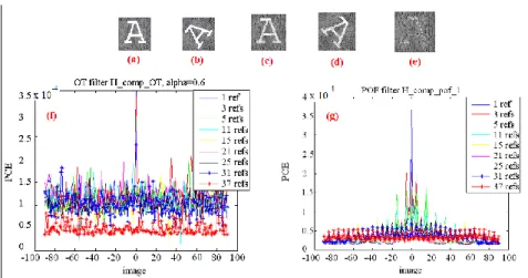
4.5. Robustness against noise

In realistic object recognition situations, some degree of noise is unavoidable. A second series of calculations was conducted in which standard noise types were added to the target image. In this section, we shall mainly consider the compromise optimal filter (OT)

OT

comp

H since it represents a useful trade-off between adapted and

inverse filters. Its tolerance to noise is also remarkable. Throughout this section, our calculations will be

compared with results obtained with filter 1

POF comp

H . At a first look at the performance of the OT filter with

noise, we consider the special case of background noise, i.e. the black background is replaced by the gray texture shown in Fig. 7 (a). Fig. 7 (b) shows the uppercase letter A with rotation (-45°).

Fig 7: (Color online) (a) Illustrating the letter A with additive background structured noise. (b) Same as in (a) with a rotation angle of -50°. (c) Illustrating the letter with structured noise. (d) Same as in (c) with a rotation angle of 50°. (e) Illustrating the letter A for a weak contrast. (f) PCEs obtained with the OT composite filter

taking α=0.6. The colors shown in the inset denote the different adapted filters depending on the number of references used. (g) Corresponding PCEs for a POF. The colors shown in the inset denote the different adapted

filters depending on the number of references used.

Fig. 7 (f) shows that the filter OT can recognize this letter only for a noisy image oriented at 0°. The results

indicate that PCE decreases as  is increased. If  is set to zero, this filter cannot recognize any letter. We also

observe that the filter OT is not robust to image rotation when the images are noisy, especially if the noise cannot be explicitly evaluated. One of the reasons we will not pursue the characterization of this filter stems from the fact that the input noise cannot be always determined in a real scene. We now exemplify the effect of background noise (applying an analysis similar to that above) by evaluating the performance of the POF (

1 POF comp

H ). A noise was also added in the white part of the letter (with reference to Figs. 7 (c) and (d)). As

illustrated in Fig. 7 (g), POF is more robust to background noise than filter OT. As mentioned previously, this is consistent with the good discrimination ability of the composite POF filters. One interesting result is that the

performances of composite filters decrease when the input image is weakly contrasted with respect to background, as evidenced in Fig. 7 (e).

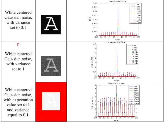
In another set of calculations, we considered the case of a Gaussian white noise on the composite POF for which the expectation value can be 0 or 1, and its variance can be set to 0, 0.1 and 1 (Table 2). Examples of noisy images are shown in the second row of Table II. Insight is gained by observing in the third row of Table 2 how the correlation results vary for different composite POFs realized with noise free reference images. As was evidenced for the standard POF, composite POFs show robustness to noise, i.e. we were able to identify noisy

images using filter 1

POF comp

H . However, it is apparent that only noisy images which have been rotated with

similar angles to the reference images have been identified.

Table 2: Calculated correlation results (third row) obtained with different composite POFs. The first row considers the numerical characteristics of the white Gaussian noise used. The second row shows a typical realization of the noisy images.

White centered Gaussian noise, with variance set to 0.1 p White centered Gaussian noise, with variance set to 1 White centered Gaussian noise, with expectation value set to 1 and variance equal to 0.1

As we have seen so far, the compromise optimal filter is robust to noise when the latter is clearly identified. However, the performance of POF is better when the characteristics of noise are unknown. It is also important to point out that the performance of both composite filters decrease when the number of reference images forming the filter is increased. It should be emphasized once more that this effect is more likely when the images are noisy.

4.6. Optimized composite filters

Next, we are interested in the design of an asymmetric segmented composite phase-only filter whose performance against rotation will be compared to the MACE filter, POF, SPOF and AMPOF. To illustrate the basic idea, let us consider composite filters which are constructed by using 10 reference images obtained by rotating the target image by 0°, -5°, +5°, -10°, +10°, -20°, +20°, +25°, respectively.

To begin our analysis, we consider the composite filter MACE. Fig. 8 presents correlation results of the letter base A (data-base obtained by rotating the A image in increments of 1° within the range (-90°,+90°)) with a composite MACE filter containing 10 reference images (0°, -5°, +5°, -10°, +10°, -20°, +20°, +25°). Here, the basic purpose is to recognize the letter A even when it is rotated with an angle ranging from -20° to 25°. In the angular dependence of the PCE value shown in Fig. 8, we can distinguish three regions exhibiting distinct correlation characteristics (referred to as A, B and C, respectively). One notices in Fig. 8 that if we restrict ourselves to region B only, correlation appears when the target image is similar to one of the reference images (Fig. 8). No correlation is observed in regions A and C of Fig. 8. The MACE composite filter is weakly robust to structured noise. Another example is shown in Fig. 9 (a) when a centered Gaussian noise of variance 0.1 is added to the input image. This figure shows the sensitivity of the MACE composite filter against this type of noise. In fact, it gives lower PCE values even with a low noise level.

Fig 8: (Color online) PCEs obtained with a 10-reference MACE when the target images are noise free. Several examples of the rotated letter A are illustrated at the bottom of the figure. The insets show two correlation

planes: (right) autocorrelation obtained without rotation, (left) inter-correlation obtained with the letter A oriented at -75° [41].

Fig. 9 (b) shows the results for the filter MACE with a structured background noise. With reference again to Fig. 9 (b) no correlation were observed even in the angular region ranging from –20° to 25° suggesting the poor correlation performances of filter MACE. We have also confirmed that the MACE composite filter is very sensitive to noise, and especially to structured noise. For this reason, we will not pursue the study of this filter in the remainder of this paper. The preceding analysis prompted us to study the composite filter performances

based on different optimized versions of the POF, i.e. filters , and . Here we

reinvestigate the identification problem of letter A in the angular region ranging from -20° to 25° by considering a 10-reference composite filter. Furthermore, we shall compare these results with those obtained using the classic

composite filter 1

POF comp

H . Parenthetically, there are similarities between the PCE calculations obtained for filters

2

SPOF

H and 2

POF comp

H with those based on filters H1SPOF and

1 POF

comp

H .

Our illustrative correlation calculations for filter 1

POF comp

H and the letter base A (data-base obtained by

rotating the A image in increments of 1° within the range (-90°,+90°)) are given in Fig. 10 (a) and (b). Shown in this figure are the PCEs for the composite POF (blue curve), the segmented composite POF (red curve), the composite AMPOF (black curve) and the composite ASPOF (green curve). We first note, in Fig. 10 (a) that the PCE values for the composite ASPOF are larger than the corresponding values when the optimization stage (see Fig. 2) has been applied to the filter. When the optimization stage has not been applied, the ASPOF PCE values are similar to the SPOF PCE values, see Fig. 10 (b) [41]. Otherwise, even if the PCEs for the composite AMPOF are larger than those for the two other filters, there is a range of rotation angle, i.e. region A, for which the segmented filter shows correlation. Also apparent is that the PCE values calculated for the segmented filter

1 SPOF

H are larger than the corresponding values of the classical composite POF 1 POF comp

H in the correlation

region A.

Fig 9: (Color online) (a) PCEs obtained with Mac composite filter and additive Gaussian centered noise of variance 0.1. (b) Same as in (a) with additive background structured noise.

In this region A, we observe large variations of the PCE values, but all the correlation values are larger than the PCE values obtained in the no-correlation regions B and C. Maximal PCE values correspond to

auto-correlation of the 10 reference images. Outside the A region auto-correlation deteriorates rapidly. From these simulations, we concluded that it is difficult to identify the letter for the three filters considered. The PCE results show significant dependence on the rotation of the target image with respect to the reference images for composite AMPOF.

Fig 10: (Color online) Comparison between the different correlations of letter A (we consider rotation angles ranging between -90° and 90°) with the 10-reference composite filters: POF (blue line), Segmented (red line), AMPOF (black line), and ASPOF (green line). (a) PCEs obtained using the optimization stage concerning the isolated pixels, (b) PCEs obtained without the optimization stage concerning the isolated pixels. (c) and (d)

represent the PCEs obtained with noised target images.

Having discussed image rotation dependence without noise of the composite filters response we now determine the impact of noise. For this purpose, we applied two types of noise to the target image, either background structured noise (Fig. 7 (a)), or a centered white noise with variance set to 0.01. Interestingly, one can see in Figs. 10 (c) and (d) the results of the PCE calculations which show the good performance of

asymmetric segmented filter . Even when noise is present, the ASPOF yields correlation in region

A. By contrast, there is no correlation in the A region with the AMPOF composite filter.

However, identification of the full letter data-base requires an increase of the reference images. This leads to the decay of the segmented filter‟s performance. Interestingly, Fig. 11 indicates that the segmented filter‟s performance is very sensitive to the number of references forming the filter. We also studied the effect of binarization on the performances of the segmented composite filter. In fact, this binarization can be an effective solution to reduce the memory size to store theses filters without altering the efficiency of the decision.

To further show the interest in using a segmented filter with respect to the saturation problem which affects the classical composite filter, we show in Fig. 12 (b) the 8-bit image of the sum (without segmentation) of the three spectra corresponding to the reference images. Fig. 12 (c) shows the corresponding sum with segmentation. Our calculations clearly indicate that the image with segmentation shows significantly less saturation than that

Fig 11: (Color online) PCEs obtained with a segmented composite filter : (a) using the energy criterion, (b) using the segmented binarized filter, (c) using filter the real part criterion, (d) corresponding binarized filter to (c).

Fig 12: Illustrating the saturation effect: (a) three 8-bit grey scale images. (b) Image obtained by a classical linear combination of the three images shown in (a). (c) Image obtained using an optimized merging (spectral

segmentation).

5. Conclusion

We now conclude with a brief discussion of the robustness of the ASPOF. In Fig. 13, we have represented the ROC curves obtained with filters (Composite-POF, SPOF, AMPOf and ASPOF) containing each 10 references (from -60° to +60°). We can see that the ASPOF filter is effective for image recognition. The ttrue recognition rate is equal to 92% when the false alarm rate is set to 0% .

Fig 13: (Color online) ROC curves obtained with 10-reference composite filters: POF (red), SPOF (green), AMPOF (purple) and ASPOF (navy blue). The sky-blue line shows the random guess [41].

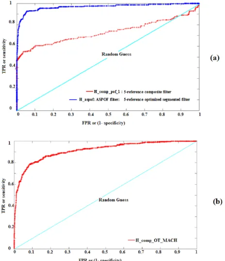
We also compared the ROC curves obtained with the ASPOF, POF, and OT MACH filters for the face recognition application (with reference to Fig. 14). We fabricated 5-reference composite filters. For the ASPOF, we used a 2-reference SPOF and a 3-reference SPOF to compute the ASPOF. The reference images correspond to -45°, -30°, -15°, +15° and +45° rotation angles. The ASPOF produces better correlation performances than the POF filter (Fig. 14 (a)). We also compared these results with the ROC curve of the OT MACH (Fig. 14 (b)). The distance between the two curves is shorter than the distance between the ROC curves of the ASPOF and POF filters but the ASPOF still indicates better performances.

Fig 14: (Color online) (a) ROC curves obtained by correlating faces of a given subject, e. g. Fig. 12 (a), with 6 other individuals with 5-reference ASPOF (navy blue) and POF (red) composite filters. The sky-blue line

shows the random guess. (b) ROC curve obtained with an OT MACH

Acknowledgments

The authors acknowledge the partial support of the Conseil Régional de Bretagne and thank A. Arnold-Bos (Thales Underwater Systems) for helpful discussions. They also acknowledge S. Quasmi for her help with the simulations. Lab-STICC is Unité Mixte de Recherche CNRS 6285.

References and links

1. A. Alfalou and C. Brosseau “Understanding Correlation Techniques for Face Recognition: From Basics to Applications,” in Face Recognition, Milos Oravec (Ed.), ISBN: 978-953-307-060-5, In-Tech (2010).

2. A. VanderLugt, “Signal detection by complex spatial filtering,” IEEE Trans. Inf. Theor. 10, 139-145 (1964). 3. B.T. Phong, "Illumination for computer generated pictures", Communications of the ACM, 18, no.6, (1975). 4. Pointing Head Pose Image (PHPID), http://www.ecse.rpi.edu/~cvrl/database/other_Face_Databases.htm

5. A. Alfalou, G. Keryer, and J. L. de Bougrenet de la Tocnaye, "Optical implementation of segmented composite filtering," Appl. Opt.

6. Y. Ouerhani, M. Jridi, and A. Alfalou, “Implementation techniques of high-order FFT into low-cost FPGA,” presented at the Fifty Fourth IEEE International Midwest Symposium on Circuits and Systems, Yonsei University, Seoul, Korea, 7-10 Aug. 2011.

7. C. S. Weaver and J. W. Goodman, “A technique for optically convolving two functions,” Appl. Opt. 5, 1248–1249 (1966). 8. B. V. K. Vijaya Kumar and L. Hassebrook, “Performance measures for correlation filters,” Appl. Opt. 29, 2997-3006 (1990). 9. J. L. Horner, "Metrics for assessing pattern-recognition performance," Appl. Opt. 31, 165-166 (1992).

10. H. J. Caufield and W. T. Maloney, “Improved discrimination in optical character recognition,” Appl. Opt. 8, 2354-2356 (1969). 11. C. F. Hester and D. Casasent, “Multivariant technique for multiclass pattern recognition,” Appl. Opt. 19, 1758-1761 (1980).

12. A. Mahalanobis, B. V. K. Vijaya Kumar, and D. Casassent, “Minimum average correlation energy filters,” Appl. Opt. 26, 3633-3640 (1987).

13. A. Alfalou, “Implementation of Optical Multichannel Correlators: Application to Pattern Recognition,” PhD Thesis, Université de Rennes 1–ENST Bretagne, Rennes-France (1999).

14. F. T. S. Yu, S. Jutamulia “Optical Pattern Recognition,” Cambridge University Press (1998). 15. J. L. Tribillon, “ Corrélation Optique,” Edition Teknéa, Toulouse, (1999).

16. G. Keryer, J. L. de Bougrenet de la Tocnaye, and A. Alfalou, "Performance comparison of ferroelectric liquid-crystal-technology-based coherent optical multichannel correlators," Appl. Opt. 36, 3043-3055 (1997).

17. A. Alfalou and C. Brosseau, “Robust and discriminating method for face recognition based on correlation technique and independent component analysis model,” Opt. Lett. 36, 645-647 (2011).

18. M. Elbouz, A. Alfalou, and C. Brosseau, “Fuzzy logic and optical correlation-based face recognition method for patient monitoring application in home video surveillance,” Opt. Eng. 50, 067003(1)-067003(13) (2011).

19. I. Leonard, A. Arnold-Bos, and A. Alfalou, “Interest of correlation-based automatic target recognition in underwater optical images: theoretical justification and first results,” Proc. SPIE 7678, 76780O (2010).

20. V. H. Diaz-Ramirez, “Constrained composite filter for intraclass distortion invariant object recognition , ” Opt. Lasers Eng. 48, 1153 (2010).

21. A. A. S. Awwal, “What can we learn from the shape of a correlation peak for position estimation?,” Appl. Opt. 49, B40-B50 (2010). 22. A. Alsamman and M. S. Alam, “Comparative study of face recognition techniques that use joint transform correlation and principal

component analysis,” Appl. Opt. 44, 688-692 (2005).

23. S. Romdhani, J. Ho, T. Vetter, and D. J. Kriegman, “Face recognition using 3-D models: pose and illumination,” in Proceedings of the IEEE 94, 1977-1999 (2006).

24. P. Sinha, B. Balas, Y. Ostrovsky, and R. Russel, “Face recognition by humans: nineteen results all computer vision researchers should know about”, in Proceedings of the IEEE 94, 1948-1962 (2006).

25. D. E. Riedel, W. Liu, and R. Tjahyadi “Correlation filters for facial recognition login access control”, in Advances in Multimedia Information Processing, 3331/2005, 385-393 (2005).

26. P. Hennings, J. Thorton, J. Kovacevic, and B. V. K. Vijaya Kumar, ”Wavelet packet correlation methods in biometrics,” Appl. Opt.

44, 637-646 (2005).

27. J. Khoury, P. D. Gianino, and C. L.Woods, “Wiener like correlation filters,” Appl. Opt. 39, 231-237, 2000.

28. A. Mahalanobis, B. K. V. Vijaya Kumar, S. Song, S. R. F. Sims, and J. F. Epperson, “Unconstrained correlation filters,” Appl. Opt.

33, 3751–3759 (1994).

29. H. Zhou and T.- H. Chao, “MACH filter synthesizing for detecting targets in cluttered environment for grayscale optical correlator,” Proc. SPIE 3715, 394 (1999).

30. A. Pe'er, D. Wang, A. W. Lohmann, and A. A. Friesem, “Apochromatic optical correlation,” Opt. Lett. 25, 776-778 (2000). 31. B. V. K. Vijaya Kumar, “Tutorial survey of composite filter designs for optical correlators,” Appl. Opt. 31, 4773-4801 (1992). 32. A. V. Oppenheim and J.S. Lim, “The importance of phase in signals,” Proc. of IEEE 69, 529–541 (1981).

33. J. L. Horner and P. D. Gianino, “Phase-only matched filtering,” Appl. Opt. 23, 812-816 (1984).

34. J. Ding, M. Itoh, and T. Yatagai, “Design of optimal phase-only filters by direct iterative search” Opt. Comm. 118, 90-101 (1995). 35. J.L. Horner, B. Javidi, and J. Wang, “Analysis of the binary phase-only filter,” Opt. Comm. 91, 189–192 (1992).

36. B. V. K. Vijaya Kumar, “Partial information filters,” Digital signal processing 4, 147–153 (1994). 37. R. C. Gonzalez and P. Wintz, “Digital Image Processing,” Addison-Wesley (1987).

38. H. Inbar and E. Marom, "Matched, phase-only, or inverse filtering with joint-transform correlators," Opt. Lett. 18, 1657-1659 (1993). 39. P. Refrégier, "Optimal trade-off filters for noise robustness, sharpness of the correlation peak, and Horner efficiency," Opt. Lett. 16,

829-831 (1991).

40. D. Casasent and G. Ravichandran, “Advanced distorsion-invariant MACE filters,” Appl. Opt. 31, 1109-1116 (1992).