Non-Conventional Numerical Strategies in the Advanced Simulation of Materials and Processes

(1)

HAL Id: hal-01007107

https://hal.archives-ouvertes.fr/hal-01007107

Submitted on 24 Apr 2017

HAL is a multi-disciplinary open access archive for the deposit and dissemination of sci-entific research documents, whether they are pub-lished or not. The documents may come from teaching and research institutions in France or abroad, or from public or private research centers.

L’archive ouverte pluridisciplinaire HAL, est destinée au dépôt et à la diffusion de documents scientifiques de niveau recherche, publiés ou non, émanant des établissements d’enseignement et de recherche français ou étrangers, des laboratoires publics ou privés.

Public Domain

Non-Conventional Numerical Strategies in the Advanced

Simulation of Materials and Processes

Hajer Lamari, Francisco Chinesta, Amine Ammar, Elías Cueto

To cite this version:

Hajer Lamari, Francisco Chinesta, Amine Ammar, Elías Cueto. Non-Conventional Numerical Strate-gies in the Advanced Simulation of Materials and Processes. International Journal of Modern Man-ufacturing Technologies, Professional Association in Modern ManMan-ufacturing Technologies, ModTech Iasi, Romania, 2009, 1, pp.49-56. �hal-01007107�

(2)

NON-CONVENTIONAL NUMERICAL STRATEGIES IN THE ADVANCED

SIMULATION OF MATERIALS AND PROCESSES

Hajer Lamari

1

, Francisco Chinesta

2

, Amine Ammar

3

& Elias Cueto

4

1_{GEM CNRS – Centrale Nantes, 1 rue de la Noe, BP 92101, F-44321 Nantes cedex 3, France}

2_{EADS Foundation International Chair, Centrale Nantes, 1 rue de la Noe, BP 92101, F-44321 Nantes cedex 3, France} 3_{Laboratoire de Rhéologie, 1301 rue de la piscine, BP 53, Domaine universitaire, F-38041 Grenoble cedex 9, France}

4

I3A, Universidad de Zaragoza, María de Luna, 7, E-50018 Zaragoza, Spain Corresponding author: Francisco Chinesta, Francisco.Chinesta@ec-nantes.fr Abstract: In this work we analyze the possibilities of

applying model reduction in the advanced simulation of materials and processes. The use of such strategies allows impressive computing time savings in the numerical simulations of complex models without degrading the solution accuracy. For this purpose we apply proper generalized decompositions of multidimensional models that can be associated to usual models in computational mechanics.

Key words: Proper Generalized Decomposition, Model reduction, Multidimensional models, Curse of dimensionality, Shape oprimization, Multi-scale modelling

1. INTRODUCTION

The fine description of the mechanics and structure of materials at the micro, nano and sub-nanometric scales introduces some specific challenges related to the impressive number of degrees of freedom required or to the highly dimensional spaces in which those models are defined. Moreover, usual models encountered in computational physics and mechanics can be transformed in multi-dimensional models allowing for very general solutions as we describe later. Despite the fact that spectacular progresses have been accomplished in the context of computational mechanics in the last decade, the efficient treatment of those multi-dimensional models needs further developments.

The brute force approach cannot be considered as a possibility for treating this kind of models. We can understand the catastrophe of dimension by assuming a model defined in a hyper-cube Ω of dimension D:

]

L L,

[

D

Ω = − . Now, if we define a grid to discretize the model, as it is usually performed in the vast majority of numerical methods (finite differences, finite elements, finite volumes, spectral methods etc.), consisting of M nodes on each direction, the total number of nodes will be MD. If we assume that for example M =10 (an extremely coarse description) and D=80 (much lower than the usual dimensions required in quantum or statistical mechanics) the number of nodes in Ω reaches the

astronomical value of 1080 that represents the presumed number of elementary particles in the universe!

We come back to the practical interest of multi-dimensional models later. In what follows in the present section we are revisiting a technique able to circumvent the curse of dimensionality issue.

1.1 Multidimensional solvers based on the Proper Generalized Decomposition – PGD -

We start writing the polynomial approximation of a generic multi-dimensional function

u x x

(

₁

,

₂

,

_⋯

,

x

_D

)

in the whole domain as:

( )

1

( )

1

( )

1 1 1 k D i N i N i i i D D k k i i k u X x X x X x = = = = = = ≈

∑

=

∑

∏

x _⋯ (1)

The coordinate x_i is not necessarily one-dimensional, but in any case it is defined in a space of moderate dimensions (1D, 2D or 3D), i.e. x_i∈Ω_i,

, 3

i

d i dï

Ω ⊂ ℜ ≤ . The model results then defined in the whole domain 1

1 D d d D + + Ω = Ω × ×Ω ⊂ ℜ ⋯ ⋯ .

One of this coordinates could be the time involved in transient models.

It is also well known that several model solutions can be approximated by a finite, and sometimes quite reduced number of functional products. Expression (1) involves N× ×M D degrees of freedom instead of the MD required in mesh-based discretization techniques.

In what follows we are describing a new advanced technique that combines a separated representation and an adaptation procedure able to build up gradually each product of functions involved in (1) until reaching the convergence. It has some resemblances with the functional approximation used within the LATIN framework, the radial approximation making use of a space-time separated representation (see [6] and the references therein) as well as with the ones employed in the

(3)

post-Hartree-Fock methods [4]. This technique has been successfully applied in a variety of linear, non linear, stationary and transient problems [1] [2] [5] [7]. In what follows we are revisiting the main ideas of such decomposition technique. For the sake of simplicity we are considering a simple multi-dimensional diffusion problem in D dimensions:

( )

(

)

] [

(

)

2 1 , , , 0,

0

D T D

u

f

x

L

u



_{∇ =}

₌

_{∈Ω =}





∈∂Ω =



x

⋯ (2)

where the general form of the right term is given by

( )

1

( )

1

( )

1 1 1 k D i m i m i i i D D k k i i k f F x F x F x = = = = = = ≈

∑

=

∑

∏

x _⋯ (3)

Such a decomposition can be performed by using singular value decomposition.

The iteration scheme used to build up the solution (1) proceeds performing an enrichment of the approximation basis at each iteration. Thus, knowing the approximation at iteration the n:

( )

1

( )

1

( )

1 1 1 k D i n i n n i i i D D k k i i k u X x X x X x = = = = = = =

_∑

=

_∑

∏

x _⋯ (4)

the approximation basis could be enriched by adding

a new product of functions 1

( )

1 k D n k k k X x = + =

∏

( )

1 1 1 k D n n n k k k u u X x = + + = = +

∏

x x (5)

that needs for the determination of the D involved functions

X

kn 1

( )

x

k

+

. For this purpose the trial function:

( )

1 1 1 k D k D i n i k k k k i k k u X x R x = = = = = = =

_∑

∏

+

∏

x (6)

is injected in the weak formulation, where

( )

n 1

( )

k k k k

R

x

≡

X

+

x

are the unknown fields of the non linear system obtained, whose size is D M× . The associated test functions are taken, again in the Galerkin’s framework, as:

( )

* * 1 1 j D k D j j k k j k k j u R x R x = = = = ≠     = _ _    

∑

_∏

x (7)

Now, as soon as the functions

R

k

( )

x

k have been

determined, the searched functions

X

kn 1

( )

x

k

+

are obtained by identifying these functions with the converged

R

k

( )

x

k functions.

This algorithm has been successfully used to solve models involving one hundred dimensions needing about ~10300 degrees of freedom if one proceeds in the finite element framework. The construction of the separated solution only needed of around 20 minutes using Matlab on a standard personal computer!. The separate representation considered in (1) only needs approximations defined in spaces of moderate

dimensions di and then integrations in such moderate

dimensional spaces because the integral of a product of functions in a hyper-domain can be written as the product of the integrals defined in the domains Ω_i.

1.2 Illustrating the Proper Generalized Decomposition construction

In what follows we are illustrating the construction of the Proper Generalized Decomposition by considering a quite simple problem, the parametric heat transfer equation:

0 u k u f t ∂ − ∆ − = ∂ (8)

where ( , , )x t k ∈Ω× × ℑI and for the sake of simplicity the source term is assumed constant, i.e. f =cte. Because the conductivity is considered unknown, it is assumed as a new coordinate defined in the interval ℑ. Thus, instead of solving the thermal model for different values of the conductivity parameter we prefer introducing it as a new coordinate. The price to be paid is the increase of the model dimensionality; however, as the complexity of the PGD scales linearly with the space dimension the consideration of the conductivity as a new coordinate allows for faster and cheaper solutions.

The solution of Eq. (8) is searched under the form:

(

)

( ) ( ) ( )

1 , , i N i i i i u t k X T t K k = = ≈

∑

⋅ ⋅ x x (9)

In what follows we are assuming that the approximation at iteration n is already done:

(

)

( ) ( ) ( )

1 , , i n n i i i i u t k X T t K k = = =

∑

⋅ ⋅ x x (10)

and at present iteration we look for the next functional product

X

_n₊₁

( )

x

⋅

T

_n₊₁

( )

t

⋅

K

_n₊₁

( )

k

that for alleviating the notation will be denoted by

( ) ( ) ( )

R

x

⋅

S t W k

⋅

. Prior to solve the resulting non linear model related to the calculation of these three functions a model linearization is compulsory. The simplest choice consists in using an alternating directions fixed point algorithm. It proceeds by assuming

S t

( )

and

W k

( )

given at the previous iteration of the non-linear solver and then computing

( )

R x

. From the just updated

R x

( )

and

W k

( )

we can update

S t

( )

, and finally from the just computed

( )

R x

and

S t

( )

we compute

W k

( )

. The procedure continues until reaching convergence. The converged functions

R x

( )

,

S t

( )

and

W k

( )

allow defining the searched functions:

X

_n₊₁

( )

x

=

R

( )

x

,

( ) ( )

1

n

T

₊

t

=

S t

and

K

_n₊₁

( )

k

=

W k

( )

.

(4)

I. Computing

R x

( )

from

S t

( )

and

W k

( )

: We consider the global weak form of Eq. (8):

* 0 I

u

k u

f

d dt dk

t

Ω× ×ℑ

∂





− ∆ − =



_∂







∫

x

(11)

where the trial and test functions write respectively:

(

)

( ) ( ) ( )

1

, ,

i n i i i i u t k X T t K k

R

S t W k

= = = ⋅ ⋅ +

+

⋅

∑

x

(12) and

(

)

( ) ( ) ( )

* *

, ,

u

x

t k

=

R

x

⋅

S t W k

⋅

(13)

Introducing (12) and (13) into (11) it results

* * ( ) I n I S R S W R W k R S W d dt dk t R S W d dt dk Ω× ×ℑ Ω× ×ℑ ∂   ⋅ ⋅ ⋅ ⋅_∂ ⋅ − ⋅∆ ⋅ ⋅  =   = − ⋅ ⋅ ⋅ℜ

∫

x x (14) with ( ) 1 1 i n i n n i i i i i i i i T X K k X T K f t = = = = ∂ ℜ = ⋅ ⋅ − ⋅∆ ⋅ ⋅ − ∂

∑

.

Now, being known all the functions involving the time and the parametric coordinate, we can integrate Eq. (14) in their respective domains I× ℑ. Integrating in I× ℑ and taking into account the notation 2 2 2 1 1 1 2 2 2 2 3 3 3 4 4 4 5 5 5 I I I i i i i i i I i i i i i i I w W dk s S dt r R d dS w kW dk s S dt r R R d dt w W dk s S dt r R d dT w W K dk s S dt r R X d dt w kW K dk s S T dt r R X d ℑ Ω ℑ Ω ℑ Ω ℑ Ω ℑ Ω  ₌ ₌ ₌       ₌ ₌ _⋅ ₌ _⋅∆      = = =        ₌ _⋅ ₌ _⋅ ₌ _⋅∆      = ⋅ = ⋅ = ⋅    

∫

x x x x x (15)

Eq. (14) reduces to:

(

)

* 1 2 2 1 * 4 4 5 5 3 3 1 1 i n i n i i i i i i i i R w s R w s R d R w s X w s X w s f d Ω = = = = Ω ⋅ ⋅ ⋅ − ⋅ ⋅∆ =   = − ⋅ ⋅ ⋅ − ⋅ ⋅∆ − ⋅ ⋅   

∫

∑

∫

x x (16) Eq. (16) defines an elliptic steady state boundary value problem that can be solved by using any discretization technique operating on the model weak form (finite elements, finite volumes …). Another possibility consists in coming back to the strong form of Eq. (16): 1 2 2 1 4 4 5 5 3 3 1 1 i n i n i i i i i i i i w s R w s R w s X w s X w s f = = = = ⋅ ⋅ − ⋅ ⋅∆ =   = − ⋅ ⋅ − ⋅ ⋅∆ − ⋅ ⋅  

∑

 (17)

that could be solved by using any collocation technique (finite differences, SPH …).

II.Computing

S t

( )

from

R x

( )

and

W k

( )

:

In the present case the test function writes:

(

)

( ) ( ) ( )

* *

, ,

u

x

t k

=

S

t

⋅

R

x

⋅

W k

(18) Now, the weak form reads

* * (n) I I S S R W R W k R S W d dt dk t S R W d dt dk Ω× ×ℑ Ω× ×ℑ ∂   ⋅ ⋅ ⋅ ⋅ ⋅ − ⋅∆ ⋅ ⋅  = ∂   = − ⋅ ⋅ ⋅ℜ

∫

x x (19) that integrated in the domain Ω× ℑ and taking into account the notation (15) results:

* 1 1 2 2 * 4 5 5 4 3 3 1 1 I i n i n i i i i i i i i I dS S w r w r S dt dt dT S w r w r T w r f dt dt = = = =   ⋅ ⋅ ⋅ − ⋅ ⋅  =     = − ⋅ ⋅ ⋅ − ⋅ ⋅ − ⋅ ⋅   

∫

∑

∫

(20) Eq. (20) represents the weak form of the ODE defining the time evolution of the field S that can be solved by using any stabilized discretization technique (SU, Discontinuous Galerkin, …). The strong form of Eq. (20) reads:

1 1 2 2 4 5 5 4 3 3 1 1 i n i n i i i i i i i i dS w r w r S dt dT w r w r T w r f dt = = = = ⋅ ⋅ − ⋅ ⋅ =   = −_ ⋅ ⋅ − ⋅ ⋅ − ⋅ ⋅ _ 

∑

 (21)

than can be solved by using backward finite differences, or higher order Runge-Kutta schemes, among many other possibilities.

III.Computing

W k

( )

from

R x

( )

and

S t

( )

: In the present case the test function writes:

(

)

( ) ( ) ( )

* *

, ,

u

x

t k

=

W

t

⋅

R

x

⋅

S k

(22) Now, the weak form reads

* * (n) I I S W R S R W k R S W d dt dk t W R S d dt dk Ω× ×ℑ Ω× ×ℑ ∂   ⋅ ⋅ ⋅ ⋅ _∂ ⋅ − ⋅∆ ⋅ ⋅  =   = − ⋅ ⋅ ⋅ℜ

∫

x x (23) that integrated in Ω×I and taking into account the notation (15) results:

(

)

* 1 2 2 1 * 5 4 4 5 3 3 1 1 i n i n i i i i i i i i W r s W r s W dk W r s K r s K r s f dk ℑ = = = = ℑ ⋅ ⋅ ⋅ − ⋅ ⋅ =   = − ⋅ ⋅ ⋅ − ⋅ ⋅ − ⋅ ⋅   

∫

∑

∫

(24)

(5)

Eq. (24) does not involve any differential operator. The strong form of Eq. (24) reads:

(

)

(

)

1 2 2 1 5 4 4 5 3 3 1 i n i i i i i i

r s

W

r s

K

r s

f

= =

⋅ − ⋅

⋅ =





= −

_

⋅ − ⋅

⋅

− ⋅ ⋅

_



∑



(25)

that represents an algebraic equation. Thus, the introduction of parameters as additional model coordinates has not a noticeable effect in the computational cost.

There are other minimization strategies more robust and exhibiting faster convergence for building-up the PGD (see [10]).

3. APPLICATIONS

In this section we are analyzing different applications of the proper generalized decomposition in computational mechanics, and in particular in the advanced simulation of material and processes, through some academinc examples.

3.1 Parametric models

We consider the 1D heat equation defined by:

( , ); _t, _x u u k f t x t x t x x ∂ ∂  ∂  −  = ∈Ω ∈Ω ∂ ∂  ∂  (26)

If k is constant, this equation can be solved for every value of k using the separated representation previously illustrated without further difficulties. Now, we are focusing on a more complicated and realistic problem. In general, for homogenous materials the thermal conductivity depends on temperature, following a linear dependence:

k=au+b (27) If we introduce this expression into Eq. (26) the resulting heat equation writes:

2 2 2 2 2 u u u u b au a f t x x x ∂ ₋ ∂ ₋ ∂ ₋ ∂  ₌   ∂ ∂ ∂ ∂  (28)

We want to solve this equation for any value of a and b. We can easily understand that the computed solution allows efficient optimization and inverse identification strategies. For that purpose the following separated representation approximation is considered: 1

( , , , )

( )

N i i i i i

u t x a b

T t X x A a B b

=

≈

∑

⋅

(29)

The numerical solution was carried out for

t

∈

[ ]

0,1

,

[ ]

1,1

x

∈ −

,

a

∈ −

[ ]

1,1

,

b

∈

[ ]

1,5

being the initial condition

u t

(

=

0, ) 1

x

= −

x

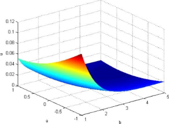
10, the temperature vanishing at both boundaries. In this example, 500 nodes were employed for discretizing each of the 4 coordinates. A mesh would have involved 5004 degrees of freedom, but using the PGD this impressive number reduces to the order of 2000. The

solution was performed in few minutes using Matlab on a personal laptop. Fig. 1 depicts the solution at point

x

=

0

at the final time

t

=

1

as a function of both parameters

a

and b.

The non linearity was accounted by assuming the conductivity given at previous iteration, i.e.

n k=au +b, where 1

( , , , )

( )

n n i i i i i

u t x a b

T t X x A a B b

=

∑

⋅

(30)

Other linearizations were analyzed and discussed in [3] and [8].

Fig. 1. Temperature at point

x

=

0

at the final time

t

=

1

as a function of both parameters

a

and

b

.

Now, we come back to the non-linear thermal model (28), with

a

=

1

and

b

=

1

, but we are focusing on its steady solution for a source term given by

(

2

)

1

f = −

β

−x ,

β

∈

[ ]

0,1

. Now, the solution is searched from the finite sum decomposition:

1

( , )

( )

N i i i

u x

β

X x B

β

=

≈

∑

⋅

(31)

The computed solution is depicted in figure 2 where we can notice, as expected, that the solution vanishes everywhere when

β

=0. 0 0.5 1 -1 -0.5 0 0.5 1 -0.6 -0.5 -0.4 -0.3 -0.2 -0.1 0 0.1

Fig. 2. Steady state temperature field

u x

( , )

β

.

Finally, we are considering the same problem, the steady state solution of a thermal model (non-linear) in which the heat source is punctual and can be applied everywhere in the domain. The thermal model is then defined as follows:

(6)

( )

u k f x x x ∂  ∂  =   ∂  ∂  (32)

where the source term writes in the present case:

(

)

( )

'

f x

= ⋅

β δ

x

−

x

(33) being

δ

() the Dirac’s mass and x' the point in which the thermal load of intensity

β

applies. As we are interested in solving the model (32) for any position of the thermal load x' and any value of the intensity

β

, we introduce the load location and the load intensity as new coordinates, searching the solution in the form:

( )

1

( , ', )

( )

'

( )

N i i i i

u x x

β

X x S x

B

β

=

≈

∑

⋅

(34)

By applying the procedure described in the previous section one could determine easily the functions

( )

i

X x

by solving a second order elliptic problem, then function

S x

_i

( ')

by solving an algebraic equation (there are not derivatives in that coordinate in the thermal model model) and finally function

B

_i

( )

β

solving another algebraic equation.

The strategy here described allows an off-line pre-calculus and very fast post-processing required in many branches of computational sciences with real-time simulation purposes.

3.2 Models defined in evolving domains

The main issue in treating models defined in evolving domains lies in the fact that

x

belongs to a domain that is evolving in time, i.e.

x

∈Ω

( )

t

. Obviously, in that case we cannot apply the procedure described previously, but the deepest difficulty lies in the fact that the space coordinate is not independent of the time coordinate.

The simplest alternative for circumventing this difficulty consists in defining the mapping between the initial space coordinates

X

∈Ω =

(

t

0 )

and the present ones

x

∈Ω

( )

t

. This mapping writes:

( )

,t

=

x

x X

. Now, the model given by

( )

(

)

,

x t

u

x

t

=

L

F

(where

_L

_{x t}_,

( )

denotes a differential operator involving the present coordinates

x

and

t

) is redefined by considering

( )

X

,

t

as new coordinates (now both being independent):

( )

(

)

* *

X,t

u

X

,

t

=

L

F

and solved by using the natural decomposition:

( )

1

( , )

( )

N i i i

u

t

X

T t

=

≈

∑

⋅

X

(35)

We are at present analyzing this approach that suggests fully Lagrangian formulation in thermo-mechanical problems. As the procedure described in

section 1.2 does not enforce the balance equations at any particular time, fully Lagrangian formulations could run as soon as the mapping

x

=

x X

( )

,

t

is well defined even in very large geometrical transformations.

In what follows we are illustrating this procedure. For this purpose we consider the filling process of a 1D porous domain by an incompressible fluid. The flow in porous media is usually modelled by the Darcy’s law that establishes the proportionality between the flow velocity and the gradient of pressures. In the 1D case that equation writes:

k dp

v

dx

η

= −

(36)

where

v

is the flow velocity,

k

is the porous medium permeability,

η

is the fluid viscosity (assumed constant) and

p

represents the pressure field. In what follows we assume without loss of generality

k

η

=

1.

Introducing Eq. (36) into the mass balance equation of an incompressible fluid that in the 1D case writes

0 dv

dx

=

(37) it results: 2 2

0 d p

dx

=

in

Ω

f

( )

t

(38)

where

Ω

_f

( )

t

represents the domain occupied by the fluid at time t,

Ω

_f

( )

t

=

] [

0,

L

_t . We assume that

] [

0

(

0)

0,

f

t

L

Ω

= =

. If the injection process is performed at constant flow rate

( )

a

, then the boundary conditions write in the case here considered: 0 0 x x

k dp

dp

a

dx

η

= =

−

=

⇒

_{= −}

(39) and

(

_t

)

0 p x

=

L

=

(40) where

L

t

= + ⋅

L

0

a t

.

The coordinate’s transformation writes:

0

1 a t

x

X

L



_⋅



= ⋅ +









(41)

where

X

∈

[

0,

L

₀

]

and

x

∈

[ ]

0,

L

_t . Now, instead of solving the problem (38) in

Ω

_f

( )

t

, we are solving this problem in the reference domain

] [

0

(

0)

0,

f

t

L

Ω

= =

. Applying the coordinates transformation (41), equation (38) results:

2 2 2 2 0 2 2 0

0 L

d p dX

d p

dX

dx

dX

L

a t









=





=





+ ⋅





_

_

(42)

(7)

which is defined in

Ω

_f

(

t

=

0)

. The boundary conditions become:

0 0 0 X

L

dp

a

dX

₌

L

a t





= −





+ ⋅





(43) and

(

0

)

0 p X

=

L

=

(44) One could try to solve Eq. (43) for each time, by considering the time t as a model parameter. Obviously as in the present case the resulting problem is two-dimensional it could be solved using any standard discretization technique (finite elements, …), however, in more complex scenarios the physical space will contain more coordinates (2D or 3D) and the coordinates transformation will imply many parameters. Thus, the resulting general parametric problem will be multi-dimensional and the use of the separated representation described in the previous section should be mandatory.

Taking into account Eqs. (43) and (44), the solution of Eq. (42) results:

( )

(

0

)

(

0

)

0

,

a

p X t

a

L

a t

L

a t

X

L

= ⋅

+ ⋅ −

⋅

+ ⋅ ⋅

(46)

in

[

0,

L

₀

] [

×

0,

T

_max

]

, that represents a separated representation:

( )

2 1

( , )

_i

( )

_i i

p X t

X X T t

=

∑

⋅

(47) with

( )

(

)

( )

(

)

1 1 0 2 2 0 0

( ) 1

X X

T t

a

L

a t

X

a

T t

L

a t

L

=





= ⋅

+ ⋅



=





_{= −}

_⋅

_{+ ⋅}



(48)

We can notice that the injection pressure

P

i goes up

in time in order to keep the solution slope constant (constant flow rate):

(

0,

)

(

0

)

i

P

=

p X

=

t

= ⋅

a

L

+ ⋅

a t

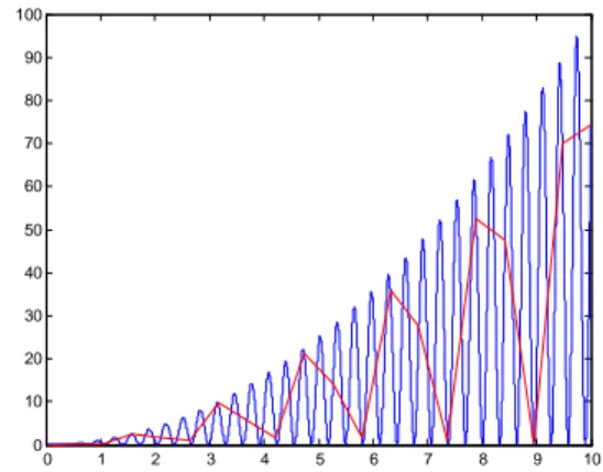
(49)

3.3 Multi-scale in time

Consider the simple model

( )

( ) ( )

2 2

2 cos

sin

du

t

dt

=

ω

−

ω

(50)

with

t

∈ =

I

] ]

0,10

and zero initial condition. The exact solution writes

u

ex

=

t

2

cos

2

( )

ω

t

. When the frequency increases, the time step must be reduced in order to capture the load evolution. Fig. 3 compares for a frequency

ω

=

10

the computed solution by using a time step of

∆ =

t

0.001

(high resolution curve) and

∆ =

t

0.5

(low resolution curve).

0 1 2 3 4 5 6 7 8 9 10 0 10 20 30 40 50 60 70 80 90 100

Fig. 3. Solution of model (50) with two different sampling times.

For accounting with the two time scales involved in the model (that we consider separated) we introduce two different times, both assumed independent:

T

= ∈

t

I

and

τ ω

=

t

∈

[

0, 2

π

]

. Thus, we postulate

( )

,

u T

τ

and Eq. (50) becomes:

( )

( ) ( )

2 2

,

2 cos

sin

du T

u

T

u

dt

T

t

T

τ

_ω

τ

ω

τ

∂ ∂

∂

=

⋅

+

⋅

=

+

=

∂

=

−

(51)

whose solution is searched by assuming the decomposition:

( )

1

( , )

( )

N i i i

u T

τ

F T G

τ

=

≈

∑

⋅

(52)

Obviously, in more complex multi-scale models involving different scales in space

( ,

_{x x ⋯}

₁ ₂

,

)

and time

( , ,

t t ⋯

1 2

)

we should write:

1 2 1 2

( , ,

,

)

u t t

⋯

x x

⋯

(53)

and in that case a separated representation seems compulsory.

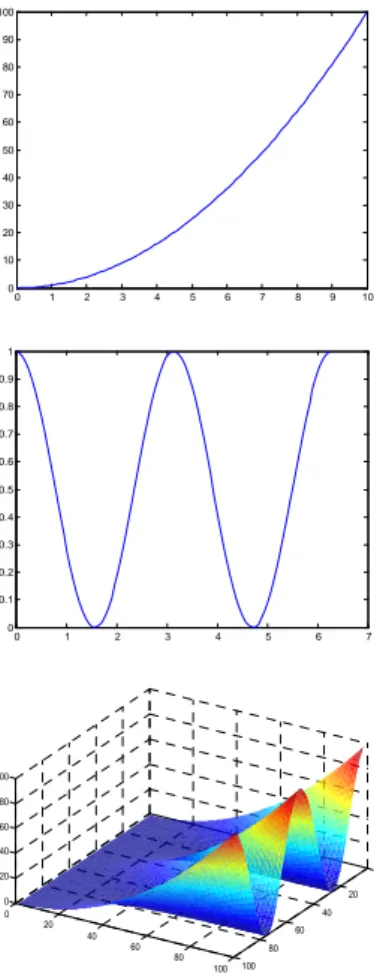
In the present case the decomposition involves a single product of functions:

( )

2 2

( )

( , )

( )

cos

u T

τ

=

F T G

⋅

τ

=

T

⋅

τ

(54)

that correspond with the exact solution, both depicted in Fig. 4. In that figure we depict also the reconstructed solution

u T

( , )

τ

.

(8)

0 1 2 3 4 5 6 7 8 9 10 0 10 20 30 40 50 60 70 80 90 100 0 1 2 3 4 5 6 7 0 0.1 0.2 0.3 0.4 0.5 0.6 0.7 0.8 0.9 1 0 20 40 60 80 100 0 20 40 60 80 100 0 20 40 60 80 100

Fig. 4. Functions

F T

( )

(top) and

G

( )

τ

(middle) associated with the decomposition of

u T

( , )

τ

in (51) and well as the

reconstructed solution

u T

( , )

τ

(bottom).

3.4 Heterogeneous materials

In this section we are focusing in the thermal models defined in heterogeneous materials. Imagine a composite material involving a matrix and a fibrous reinforcement. A typical

representative volume showing the microstructure heterogeneity is depicted in figure 5.

Fig. 5. Microstructure of a composite material

Now, in order to apply the PGD one should perform a separated representation of the thermal conductivity, allowing for an efficient thermal simulation, i.e.

( )

1

( )

P i i x y i

k

K x K

y

=

≈

∑

⋅

x

(55)

This separated representation can be performed by applying the SVD (singular value decomposition) to the matrix containing as entries the image pixels. However, because the irregular distribution of the inclusions the number of sums in (55) becomes very high. Different possibilities exist to alleviate this representation some of them are being analyzed at present. A first possibility lies in considering only a reduced number of the modes of the SVD. The computational cost is significantly reduced and sometimes the precision is not too much degraded. Figure 6 depicts the image reconstruction for different number of sums in (55).

Fig. 6. Reconstructed microstructure for

P

=

23

(left) and

46 P

=

in (55).

Another possibility lies in the substitution of each cercle by a square parallel to the coordinate axes, whose area equals the one of the associated circle. Eq. (56) represents a generic rectangle:

[

x x

_a

,

_b

] [

y y

_a

,

_b

]

∈

×

x

(56)

Now, we define the characteristic function:

( )

,

0

1

0

a b

if

s

a

s

if

a

s

b

if

s

b

χ

<





=



≤ ≤



_>



(57)

Uisng this notation, the square defined in (56) can be represented in a separated form by:

( )

, ,

a b a b

x x

x

y y

y

χ

×

χ

.

Obviously, if the representative volume contains P inclusions, each one represented by a square, the separated representation (55) will contain P sums. Obviously, all these approaches imply the solution of a thermal model for each representative volume (as soon as the microstrucvture evolve, the thermal conductivity is modified and then a new solution of the thermal model is required). If we consider a stochastic nature of the microstructure many realizations of the microstructure must be solved. One possibility for alleviating this task consists of considering the representative volume composed of a certain number of cells related to a grid of the representative volume as depicted in figure 7. Now, rather than solving a thermal model for each possible microstructure (represented by the different values of the thermal conductivity in each cell), we are introducing the thermal conductivity of each cell as an extra coordinate. In the example depiected in Fig.

(9)

7 the model will be defined in a space of dimension 27 (the x and y space coordinates and the

5 5

×

cells thermal conductivities).

Fig. 7. Cellular microstructure of the representative volume.

Thus, the solution is searched under the form:

( )

1,1 5,5 1,1 1,1 5,5 5,5 1

( , ,

,

)

( )

(

)

(

)

N i i i i i

u x y k

k

X x Y y

K

k

K

k

=

≈

∑

⋅

⋯

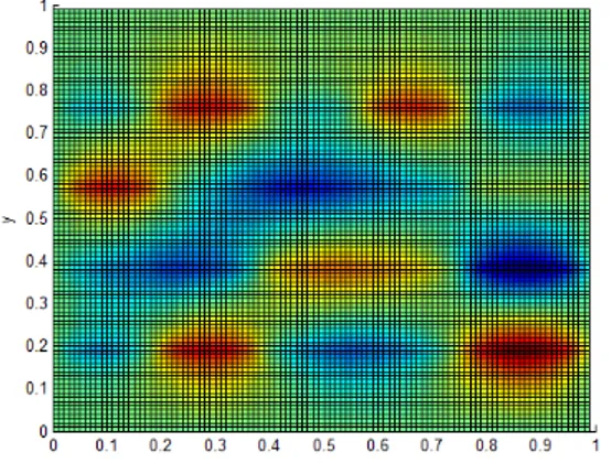
(58)

Thus, the termal field for any possible microstructure only needs the solution of only one multidimensional problem, solution that can be performed efficiently by applying the PGD. As soon as the solution (58) is computed, the thermal field for any microstructure realization is obtained by substituting the known conductivities of each cell in Eq. (58). Thus, the thermal field related to the microstructure shown in Fig. 7 is depicted in Fig. 8 (a simple boundary condition

u

(

x

∈∂Ω

,

k

_1,1

,

_⋯

,

k

_5,5

)

=

x

was enforced)

Fig. 8. Thermal field associated with the microstructure depicted in Fig. 7.

4. CONCLUSIONS

This paper explores some possibilities related to the use of Proper Generalized Decomposition in the advanced simulation of materials and processes. This novel discretization technique allows the efficient solution of highly multidimensional models by circumventing the redoubtable curse of dimensionality that mesh based discretization techniques suffer.

As soon as an efficient solver for multidimensional models is avalaible, many models of computational

mechanics can be rewritten in higher dimensional spaces. Thus one could for example compute the thermal field for any value of the thermal conductivity (as illustrated in this paper for homogeneous and heterogenous materials) simplifying inverse identification of optimization; compute the solution for any geometry for addressing evolving domains or shape optimization; or addressing multi-scale models in space or time encountered in many manufacturing processes, as for example the ones involving ultrasons, microwaves or localization.

5. REFERENCES

1. Ammar, A., Mokdad, B., Chinesta, F., Keunings, R. (2006). A new family of solvers for some classes of multidimensional partial differential equations encountered in kinetic theory modelling of complex fluids. J. Non-Newtonian Fluid Mech., 139, 153-176. 2. Ammar, A., Mokdad, B., Chinesta, F., Keunings, R. (2007). A new family of solvers for some classes of multidimensional partial differential equations encountered in kinetic theory modelling of complex fluids. Part II: Transient simulation using space-time separated representations. J. Non-Newtonian Fluid Mech., 144, 98-121.

3. Ammar, A., Normandin, M., Daim, F., Gonzalez, D., Cueto, E., Chinesta, F. Non-incremental strategies based on separated representations: Applications in computational rheology. Communications in Mathematical Sciences, In press.

4. Cancès, E., Defranceschi, M., Kutzelnigg, W., Le Bris, C., Maday, Y. (2003). Computational quantum chemistry: A primer. Handbook of Numerical Analysis, Elsevier, Vol. X, 3–270.

5. Chinesta, F., Ammar, A., Lemarchand, F., Beauchene, P., Boust, F. (2008). Alleviating mesh constraints: Model reduction, parallel time integration and high resolution homogenization. Comput. Methods Appl. Mech. Engrg., 197, 400-413.

6. Ladeveze, P. (1999). Nonlinear computational structural mechanics. Springer, NY.

7. Mokdad, B., Prulière, E., Ammar, A., Chinesta, F. (2007). On the simulation of kinetic theory models of complex fluids using the Fokker-Planck approach. Applied Rheology, 17/2, 26494, 1-14.

8. Pruliere, E., Chinesta, F., Ammar, A. On the deterministic solution of parametric models by using the proper generalized decomposition. Mathematics and Computer Simulation. Submitted.