Tidal accelerations and dynamical properties of three degrees-of-freedom pendula

Should thelaws of gravitation be reconsidered 1 Héctor A. Munera, ed. (Montreal: Apeiron 2011)

Tidal accelerations and

dynamical properties of

3-df pendula

René Verreault

Department of Fundamental Sciences University of Quebec at Chicoutimi 555, Boul. de l'Université

Saguenay (Quebec) Canada G7H 2B1

Rene_Verreault@uqac.ca

1 Introduction

In the abundant litterature on the spherical pendulum and in particular on the Foucault pendulum, the system generally con-sidered consists of a point mass constrained to move on a spheri-cal surface, when not projected on a horizontal plane. However if one is interested in studying very subtle perturbations of the spherical pendulum, it is necessary to deal with the "physical pendulum" altogether. An oscillating mass with 3-D extension usually lacks rotational symmetry about the spin axis, which is the line joining the instantaneous suspension point and the centre of mass, hereafter called the "bob", of the pendulum. The spin constitutes therefore an inherent third degree of freedom (df) for every physical pendulum. For the usual Foucault pendulum where a heavy mass is suspended by a metal wire, the third df takes the form of a torsion pendulum with a restoring torque originating from the elastic properties of the wire. However, for the ballborne pendulum of the Allais (paraconical) or Goodey type, [1][2] the spin motion is more complicated since there is es-sientially no restoring torque, except for a very small rolling fric-tion torque at the area of contact. Spin mofric-tion is nevertheless

ob-served in practically every run, but to the author's knowledge, nobody, including Allais and Goodey, [1] has published on the subject. The experimental data suggest that there is a connection between the ellipticity of the bob orbit, the precession of the el-lipse and the growth of an angle of spin. The purpose of this arti-cle is to study that relation and to try to find out whether, accord-ing to classical mechanics, it plays a role in the influence of the relative motion of the Earth, the Moon and the Sun on a 3-df pendulum.

2 Theory

In order to estimate the possible influence of the Moon, say, on the pendulum motion through tidal effects, one may first con-sider the main tidal components over a few days interval. On such a short arc compared to the whole Earth orbit, the motion of the Earth-Moon centre of mass is considered rectilinear enough to be the origin of an inertial system. However, the centre of the Earth is also moving at 0,73 Earth radius from that origin. If ΩM is the orbital angular velocity of the Moon, the centripetal accelera-tion of the Earth centre is 0,73rΩM2 , which, unlike the surface cen-tripetal acceleration rΩ2 _{, is neither constant nor included in the} apparent gravitational acceleration g at the Earth surface. The three orders of magnitude ratio between the two justifies taking the Earth centre coordinate system as inertial. The ΩM2 term could be added in a refined study if necessary.

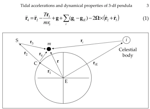
As already pointed out by Munera, [3] the suspension point S is not a good laboratory reference for pendulum motion since, in a ballborne or paraconical pendulum for instance, S wanders somewhat erratically on a flat surface when the bob is moving. Even for a standard Foucault pendulum, the true height of the in-tersection point S between the vertical and the wire centre line changes with the amplitude and with the azimuth (suspension anisotropy) of the oscillation. This is namely responsible for the Kamerlingh-Onnes ellipses and precessions which are observed in practically every physical pendulum. [4] Therefore, experimen-tal measurements are best made with reference to some alidade centre C which is fixed relative to the earth surface. Figure 1 shows the various vectors pertaining to that situation. The equa-tion of moequa-tion in the laboratory system takes the form:

(

2 3

)

3 3 2 4

g

(

g

g

)

2

Ω

r

r

r

r

r

ɺ

ɺ

ɺ

ɺ

ɺ

ɺ

=

−

+

+

∑

−

−

×

+

i iE i

mr

T

(1) m i E C S r_iE r₃ r r_i r₄ r₂ r₁ Celestial body

Figure 1. Pendulum geometry referred to the centre of the Earth.

Equation (1) is equivalent to Allais' Equation (4), p. 127 of his book, [5] except for a change of the laboratory origin in favor of the alidade centre C instead of the suspension point S.

It must be said at this point that the normal tidal effect due to the body i as the Earth rotates amounts to a periodical tilt of the local vertical at the ith _{synodic rotation period of the Earth,} eventually including some harmonics. For a 20-meter Foucault pendulum at mid latitudes, the centre of the elliptical bob orbits will describe its own ellipse with semi-axes of the order of 0,1 mm, under the influences of the Moon and the Sun. Such a tidal tilt would decenter a 1-meter pendulum by approximately 50 µm.

3 Precession through gyroscopic effect

The airplane pilot's way of looking at gyroscopic effects is: if you want the horizontal axis of a rotating disk (propeller) to point upwards as per pushing on the bottom part of the disk plane, the effect will be as if the same push were applied 90° farther in the rotation direction. A cw rotating propeller as seen by the pilot will precess toward the right on a nose-up command, and vice-versa. This reasoning can be applied to the pendulum in each half-cycle as the Earth deviates the horizontally lying axis of swing at a steady rate.

Let us assume that a pendulum at the equator is swinging in a north-south vertical plane, after a start from the southern hemisphere at t = 0. The angular momentum vector about S is pointing eastwards for the first half-cycle. The Earth rotation is commanding "nose-down", so the pendulum will precess to the left. On the next half-cycle, the pendulum angular momentum is now point west and the Earth commands "nose-up". The result is a precession to the right exactly cancelling the effect of the preceding one. Hence the principal normal tidal effect due to the Moon and observable in the laboratory is:

1° from Section 2: an extremely small alternating tilt of the vertical with a 12,4-hour period and an amplitude of ~10-6 _rad;

2° from above: absolutely no net precession due to that tilt.

4 Precession and elliptical orbits due to perturbations at the pendulum frequency ω

Perturbations having a rigid phase relation with the pendu-lum oscillation are especially prone to induce parametric amplifi-cation of some of the parameters. For instance, parametric ampli-fication of the b-axis results in the growth of elliptical motion. Us-ing perturbation methods, Pippard wrote an illuminatUs-ing paper on that subject. [6] He considers, on the right-hand side of the dif-ferential equations, a perturbing force resolved into four compo-nents as follows (index c for cosine, and so on):

t

F

t

F

_ac

cos

ω

+

_as

sin

ω

along the major axis, (2a)

t

F

t

F

bc

cos

ω

+

bs

sin

ω

along the minor axis, (2b)

It turns out that the force component in phase with the mo-tion on any axis generates elliptical momo-tion, while a component at 90° out of phase with the motion on any axis generates preces-sion. This is just a generalization of what happens with the Fou-cault precession, where the Coriolis force is at 90° out of phase with the motion along the major axis. More precisely, the preces-sion angular velocity is given by

ω

ε

F ma

Fbs ac

p =( + ) 2

Ω (3)

where

ε

=

b

a

; and the rate of growth of ellipticity is given by

ω

ε

5 Lunar tidal effects on the pendulum

In Equation (1), the tidal term from the Moon is

(

g

_M

−

g

_ME

)

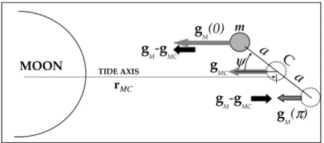
. It is however pertinent to separate, as Allais did, the tidal contri-butions at various frequencies: first a rapidly varying term at the period of the pendulum T=2π/ω , and second, a slowly varying term involving the Earth synodic period TE ≈ 24,8 h and the Moon synodic period TM ≈ 29,5 d. For that purpose, let us define an intermediate point C as the centre of the pendulum orbit, which coincides with the instantaneous rest point of the bob if the swing amplitude were zero. Refining Allais' formalism, one has

) ( ) ( ) (g_M −g_ME = g_M −g_MS + g_MS −g_ME (Allais) (5a) or (g_M −g_ME)=(g_M −g_MC)+(g_MC −g_MS)+(g_MS −g_ME). (5b) Allais' last term above has already been dealt with in Section 3, at least for the Earth rotation period. It has been found that it results in tilting the vertical. So, added to any motion of the sus-pension S at frequencies well away from pendulum resonance, point C will describe a tiny ellipse, submillimeter in size, which could possibly be modulated at the longer lunar obital period TM. That tilting should be measurable. There remains now the short-period term, which can be interpreted with the help of Figure 2.

MOON ψ m r_MC TIDE AXIS a a C g M-gMC g M-gMC g MC g M(0) g M(π)

Figure 2. Tidal accelerations acting at the pendulum frequency (the vector mod-ules have been exagerated for clarity).

The main tidal accelerations experienced during the Earth rotation are indeed very slightly modified along the way by the fact that the pendulum oscillation superimposes the extremely small swing motion to the rapidly changing Moon-pendulum distance. Let the Moon-pendulum distance increase rapidly due to the Earth rotation entraining the laboratory away from the Moon and/or to the Moon orbit gaining altitude after its perigee.

The average acceleration gMC decreases in a "smooth" fashion

while the instantaneous bob acceleration

g

M decreases more

rapidly when the swing has a component away from the Moon and less rapidly when the swing is toward the Moon. This phe-nomenon amounts to another tidal contribution exactly in phase with the pendulum swing along each axis (cosine terms in Equa-tion 2). It could be measured, if large enough, in the lab coordi-nates. Concerning the possibility of ellipse generation by the tidal tilting action, it is clear that the tilt tidal frequency is far too low to induce parametric amplification of b and, moreover, it is not commensurate with the pendulum period. So, the answer is no.

Allais has properly recognized those situations on page 127 of his book, [5] where he correctly neglects his term "(grad_SU_i−grad_TU_i) = déviation de la verticale" [(gMS-

g

ME) of

Equation (5) above], which is now known to induce neither pendulum precession nor ellipse formation in the lab coordinates. He retains only his term "(gradGUi−gradSUi)" [(

g

M- gMS) of

Equation (5) above].

Admittedly, he made an estimation of this term without con-sidering the instantaneous rapid change in the Earth-Moon dis-tance (from one to a few kilometers per pendulum period). The present author has addressed this problem in an unpublished paper. It turns out that for uniform and rectilinear relative Moon-pendulum motion, the result would be identical with the situa-tion at rest, since over a finite number of swing periods, the aver-age of the instantaneous positions of the bob and the averaver-age po-sition of the ellipse centres coincide. On the other hand, at the ex-treme situations of relative acceleration, namely with the Moon near its perigee or apogee and with the laboratory at the latitude of a subsolar or sublunar eclipse point, the means of bob posi-tions and ellipse centres no longer coincide. That non inertial tidal effect is at most of nearly the same magnitude of the linear one, mainly canceling it in the receeding lab extreme or doubling it in the other extreme. To find out how the pendulum motion would be affected in the non accelerated case, let us assume the simpler situation of fixed Moon-pendulum distance and extremal lateral accelerations (polar experiment with equatorial eclipse).

From Equations (2) and Figure 2, one finds Fas =0 ; Fbs =0;

ψ

cos ) ( _{Mmax MC} ac m F = g −g ; (6a)

ψ

sin ) ( _{Mmax MC} bc m F = g −g . (6b)

Equation (3) states that there is no precession without the presence of an ellipse. Fbc, which is the tranverse component

when the bob is at the end of the a-axis, generates an ellipse when there is none or amplifies an existing positive one. At the same bob position, the velocity along the b-axis is maximal if there is an existing ellipse and Fac is tranverse to that velocity, which creates

a precession of that ellipse.

Therefore, this submicroscopic tidal effect at the lab scale (or swing scale) will theoretically create no precession directly but the onset of an ellipse if there is none. Once there is an ellipse, a precession speed will grow up proportional to the b-axis.

For the other extreme situation of an equatorial experiment with Sun and Moon at zenith, there is no perturbing force in the orbit plane. Classical mechanics can only affect the period.

In short, Allais estimate is confirmed as to the magnitude of his tidal accelerations, namely as being 8 orders of magnitude be-low the values of F_µν /m that would account for the observa-tions (µ = a,b; ν = c,s) .

Of course, this last analysis may look very academical since this submicroscopic tidal effect originating from the Moon or any other celestial body can certainly not be measured by today's technology. But the situation may be different if large perturbing masses lie very close to the pendulum, like a concrete column or obese observers… In principle, an asymmetrical mass distribu-tion around the pendulum leads to an anisotropy of the gravita-tional field potential well in which the pendulum evolves. For in-stance, suspension anisotropy can be analysed in terms of a very weak saddle-like field at point C, superimposed to the ideal spherical well. After all, Cavendish's torsional balance works on the principle of a saddle-like gravitational field. The question arises whether such a rotating saddle-like field originating from celestial bodies (space anisotropy) and from Earth rotation is suf-ficient to explain the tendency of the pendulum azimuth toward the low-energy axis. It seems that classical mechanics fails to an-swer the question so far.

6 The spin degree of freedom

In accelerated reference systems, nonlinear phenomena real-ize a coupling between otherwise independant df. The rigid body ballborne physical pendulum may be considered with 5 df, if the vertical motion of the suspension plane is neglected :

• 2 high-energy df of oscillation about the instantaneous suspension contact point,

• 1 medium-energy df of spin, with essentially no restoring torque, about a line through the moving contact point and the centre of mass,

• 2 low-energy df of horizontal translation of the average position, over a integer number of periods, of the contact point on the suspension plane.

On the other hand, one may find for the standard Foucault pen-dulum as many of 12 df:

• the 2 usual high-energy angular oscillation df about a slowly moving point in space;

• 4 medium-energy df : 1 spin with restoring torque about the wire centre-line; 2 transient orthogonal wobbling mo-tions of the bob about the insertion point of the wire near its upper surface; 1 transient longitudinal wire vibration mode;

• 6 low-energy df: 1 long-term low-energy df being the pen-dulum length affected by temperature, and affecting the period; 3 long-term low-energy df of horizontal and vertical oscillation of the suspension point; 2 transient transversal vibration modes of the wire.

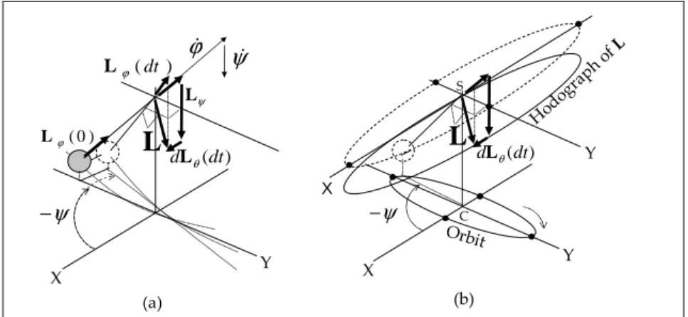
It is interesting to note that, once the initial bob wobbling and wire vibrations have died out, the bob-wire unit seems to act as a rigid body, at least for a time scale larger than the wobble natural frequency. The perturbing effect of the spin can be best visualized at the beginning of a swing cycle when the swing an-gular momentum is zero. Let us assume then that the pendulum has the spin velocity

ϕ

ɺ_{. Momentarily, the spin momentum}

consti-tutes by itself the total angular momentum of the pendulum. In Figure 3a, the gravitational torque imgl

θ

_max =dL_θ /dt tends to bring the vector

ϕ

ɺ _{parrallel to the vertical axis.}

How-ever, the Z-component of the angular momentum must stay con-stant. Indeed,

ϕ

and

ψ

do not appear explicitly in the

Lagran-gian for an isotropic pendulum with no spin restoring torque. For such ignorable variables, the vertical components of angular mo-mentum constitute constants of the motion. [7] Even with a small restoring torque −D

ϕ

or with suspention anisotropy being a very weak function of the azimuth

ψ

,

ϕ

ɺ _and

ψ

ɺ _{are practically}

constant over one period.

(a) ψɺ Y X ) (dt dL_θ ) ( dt ϕ L ) 0 ( ϕ L ϕɺ ψ −

L

Y X ) (dt dLθ ψ −

L

H odog raph ofL Orbit X Y (b) ψ L S C

Figure 3. Perturbation originating from the spin. The horizontal scale has been exagerated for clarity.

Consequently, the allowable motion at the start is in an hori-zontal plane instead of downwards as commanded by gravity. The support will therefore provide a reaction torque along the vertical axis corresponding to Lψ and

ψ

ɺ in Figure 3a. The verti-cal momentum component associated with

ψ

ɺ _is

ab L L L_ψ =− _ϕcos

θ

+ , ab ab I

L = _ψ

ψ

ɺ _{measures the vertical component of the orbital}

angu-lar momentum associated with an elliptical orbit. It appears in Figure 3b as the height, in momentum units, of the hodograph of

L above (or below, as here) the suspension point S. ab

m L

L

L_ab =± (

θ

)sin

θ

≈± (

θ

_max)⋅

θ

_max =

ω

, (sign of b). The bob ,then, starts an horizontal motion towards the nega-tive X, thus initiating an elliptical orbit. In the above example,

4 2 max 2 2 10 4 5 2 ≅− =−

ϕ

≈− ⋅ −

θ

ϕ

ε

ψ ϕ _ɺ ɺ ɺ l r I I s-1 ₍₇₎

In fact, the rather large value of

ε

ɺ _{takes the form of a short}

side-kick impulse at the begining of the cycle, so that the ellipse remains at first quite narrow. For after a time dt of a few millisec-onds, the increment dLθ become larger than the spin momen-tum and overrides it, starting to bring the bob down. From then on, it is the spin that becomes the peturbing agent for the princi-pal angular momentum L=L_ϕ +L_ψ +L_θ.

Since L=r3×v must at all times be perpendicular to the

ra-dius vector r3 and to the velocity

v

of the bob along the

right-handed orbit of Figure 3, it points slightly below the horizontal plane (dotted ellipse) containing the suspension point as the momentum origin. In practice,

θ

max being small, the hodograph

of L lies very close to that plane. Moreover, the part of L_ψ which lies above the origin represents the perturbation due to the spin, namely a precession of the orbit at the rate

ψ ϕ

ϕ

ψ

ɺp =−ɺI I s-1. (8)

(a) (b) (c)

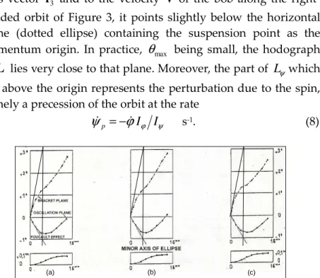
Figure 4. Monthly (a) and semi-monthly (b and c) averages of precession angles, spin angles and minor axis values within 14 min from start. The angle units are grads. The Foucault effect is ψɺF=−2,94 grads (−2,64°) per 14 minute run

(−0,55⋅10−4 s-1_{). [8] Adapted from Allais' memoir to the NASA. [9]}

7 A new interpretation of Allais' results

For the ballborne pendulum with no restoring torque, Equa-tion (8) should be reversible, so that the onset of a precession should generate a corresonponding spin. This can be seen in

Al-lais's Graph IV of its memoir for the NASA, [9] reproduced here in Figure 4. Allais' so-called "gyrostaticity coefficient"

ψ ϕ

θ

ϕ

θ

γ

=

I

I

=

I

max

I

. So, at the start of Allais' experiment,

325

,

0

max

=

=

γ

θ

ψ ϕ

I

I

, making the slope of the spin angle

("bracket plane" in Figure 4) 3,08 times steeper than the negative of the Foucault slope. The tangent lines added on Figure 4 illus-trate the very good agreement with the above theory.

When spin kinetic energy or minor axis kinetic energy are growing, the energy must come either from a separate excitation or from a coupling between degrees of fredom. Combining Equa-tions (7) and (8), one has

ε

ψ

ϕ

ɺ=cϕψ ɺp+cϕεɺ (9)

From Equations (7) and (8), c_ϕψ =c_ϕε =−3,08 .

Representing as in Figure 3b the momentum space with an origin at S, it can be seen that the precession and ellipse growing contributions from the spin are separated by the origin level: ccw precession and ccw elliptical increments belong to the positive (above S) half of momentum space, and vice-versa. The coupling involved in Equation (9) obviously comes from the motion con-straint that the vertical component of angular momentum must remain constant if

ϕ

and

ψ

are ignorable variables. Although the Airy precession speed, [10] not shown in Figure 3, is usually too small to be illustrated for a long Foucault pendulum, it is far from negligible in Allais' paraconical pendulum, where l2 _{is O(1)} m2_{. Equation (9) should then be re-written:}

ε

ψ

ψ

ϕ

ɺ=cϕψ(ɺF + ɺA)+cϕεɺ , (10) with

ψ

ɺ_A =(3/8)

ω

ab/l2_{. (11)} It is interesting to note that, in accordance with Equation (10) where c_ϕε <0, the maximum growth rate of minor axis coincides with a minimal slope of the spin curve in Figure 4.

Allais' data on swing amplitude are not precise enough to enable an assessment of energy transfer from that df to the other ones. However, it is found that the only precession contribution other than Foucault precession (circular anisotropy characterized by non degenerate circular eigenmodes) is Airy precession, [11]

and that the external influence from any source takes the form of linear (suspension or space) anisotropy characterized by non de-generate linear eigenmodes with different periods for swing di-rections at 90° from one another. Allais states indeed in his equa-tions, [11] that the precession angles that he observes outside the Foucault effect are solely explained by the Airy effect on the ellip-ses generated from suspension and/or space anisotropy.

However, from the minor axis value of Figure 4 after 14 min-utes (

ε

ɺ=0_{), Equation (11) gives}

F

A

ψ

ψ

ɺ =_1,1⋅₁₀−4_s-1=−_2,0ɺ _,

giv-ing, after 14 min, 5,4 grads of Airy precession. But from the ex-perimental slope of the precession angles at that time,

F

ψ

ψ

ɺ _0,5ɺ

exp≈− , allowing for other precession contributions.

Roughly 4 grads of Airy effect are missing.

There should also be an "Airy-like" contribution arising from the asymmetry of the ellipsoid of inertia, whose axes stay within a few degrees of the swing azimuth. From Allais' asymmetry data, [12] the disk-shaped vertical bob lies indeed in a plane close to the major-axis azimuth. The resulting longer swing period in the ma-jor axis direction should then enhance the Airy effect, contrary to what is observed in Figure 4. The missing positive Airy-like pre-cession speed that is due to anisotropy axes which are somewhat bound to the swing azimuth, is obviously transferred to a negative spin contribution 3 times as large which is subtracted from the Foucault-induced spin (9,0 grads after 14 min). The missing 6,3 spin grads can therefore account for +2,15 grads of precession, which is rather close to the missing 2,5 grads of Airy effect alone. Allais seems to affect space anisotropy solely to changes in minor axis. There might also be a direct precession effect which does not explicitely show up in building ellipses, and which may be

masked by the buffering behavior of the spin df. That would be consistent with eclipse effects on torsion pendula. [13] [14]

8 Spin characteristics of the Foucault pendulum

Because of the spin restoring torque of the Foucault pendu-lum, a steady spin-inducing perturbation cannot build up spin angle indefinitely. Its action in a given direction is limited to a fraction of the spin period. Hence, the coupling constants be-tween spin angle, minor axis swing amplitude and precession

angle must be much smaller than with the short and rigid ball-borne pendulum. Thanks though to the high precision video re-cording of pendulum motion achieved in the 2001 Chicoutimi experiment, [15] the first evidence of spin-orbit coupling with a long Foucault pendulum has been demonstrated by the author. The observations involve the simultaneous imaging of an array of luminous spots on an alidade fixed to the laboratory floor at the same height as the bob top surface, and a similar array of lumi-nous spots attached to the top surface of the bob itself. Strictly speaking, this system records the relative motion of the insertion point of the flexible wire into the bob top surface. Through the use of deflecting mirrors, the camera, no matter its size, has a bird's view from a point ~2 cm beside the suspension point, thus measuring essentially parallax free angles from the vertical. In practice, once the initial wobbling and string modes have died out, it is assumed that the motion of the centre of mass is re-corded. Moreover, since the deflecting mirror is solidary with the suspension rig, suspension motion appears as a relative alidade motion in the image. In the 2009 Gifu experiment (Japan), alidade pseudo-oscillations in phase with the pendulum could demon-strate suspension-beam flexion and torsion as small as 10-7 _{rad for} a swing amplitude of 0,015 rad. That ended up in measurable pendulum anisotropy in the form of orthogonal swing periods differing by 3 parts in 10-5_{. Similarly, in the above mentioned} 12-hour Chicoutimi experiment, the direct lunisolar tide effect could at most be seen as a complete conical sweep of the vertical along a 0,4 mm-radius circle on the floor. [15] Comparing it with the expected value in Section 2, this may include a small strain of the hosting cathedral as the Sun shines around the stone walls.

That particular experiment was started with a one-turn spin angle in order to see eventual interactions between spin and pre-cession. In aftermath, the author argues that the Longden corked wire anisotropy can be eliminated this way, [16] since the even-tual anisotropy axes aceven-tually swept an angle range between π and

π/2 for the totality of the experiment (spin time constant = 16 h). Incidentally, beside spin-orbit coupling and a Foucault effect of

Ω

_F

=

−

11

,

25

°/h , the precession angle of that 17,4 m long pendulum showed ocsillations components in phase with the 3 most important harmonics of the tide in the nearby Saguenay River, albeit with different amplitude ratios (as Allais also found

out). Needless to say, both the direct lunisolar influence and the gravitational influence of the alternating water mass in the river fall short of explaining the measured accelerations by 8 and 4 or-ders of magnitude respectively. The data fit the precession equa-tion below to ±15%, except for the last spin-orbit term: ±30%. N.B.: The precession speed oscillation due to the 360° spin had a

non negligible amplitude : 2,7

max = ϕ ϕ = ϕ

ω

ψ

ɺ A _{°/h !} ); cos( ) 2 cos( ) cos( ) cos( ) cos( 6 6 6 2 2 2 1 1 1 ϕ ϕ ϕ ψ ψ

δ

ω

δ

δ

ω

δ

ω

δ

ω

ψ

+ + + Ω + + + + + + + Ω = t A t A t A t A t A t F T T T F Aψ: anisotropy term

[

]

[

]

[

]

[

]

[

]

[

2

]

2 1 1 s) 212 2 ( cos 03 , 0 9 , 4 h) 6 1 2 ( cos 35 , 0 h) 1 , 4 2 ( cos 38 , 0 h) 2,4 1 2 ( cos 05 , 1 2 , 2 h) 8 , 24 2 ( cos 68 , 1 h 32 360 π π

π

π

δ

π

π

δ

π

π

ψ

+ ° + + ° + − + ° + + + ° + + ° + ° − = t t t t t t Semi-minor axis -1 0 1 2 3 4 0 9 18 27 36 45 Cycle b ( m m )

Figure 5. Effect of an initial spin on a 7,2-meter long Foucault pendulum in Ta-hiti. The bob design allowed for rapid spin damping over a few swing cycles.

A recent experiment in Tahiti (2010) is now in preliminary processing using a new proprietary pendulum analysis software. Different parameters are obtained at every half cycle with a preci-sion unattained before. That experiment could be run with no spin by feeding the wire through the bob in a fixed capillary and then clamping it underneath. The wire torsion was hindered by friction inside of the capillary. Figure 5 shows the correspondence between minor axis and precession speed after an undesired 10° initial spin. The 7,2-meter pendulum had a spin period of 8,5 swing periods. A +3-mm b-axis yields a ccw precession speed increment of 0,8 °/h, which fades out within ~30 swing cycles. It reaches up to 20% of the ccw, 4,53 °/h, Foucault effect in Papeete.

9 Conclusion

It can be seen from the above that the spin df plays an essen-tial role in the short ballborne pendulum. It may yield a buffering action that will mask eventual direct precession contributions arising from an external pendulum perturbation. In that sense, Allais might have erroneously reserved exclusively minor axis changes to all the external influences, explaining his precession observations merely by the subsequent Airy effect. The long Fou-cault pendula show unexplained precession contributions orders of magnitude larger than the practically negligible Airy preces-sion. Direct precession reveals the existence of circular anisotropy in the surrounding field, which appears consistent with many ob-servations on torsion pendula.

The author acknowledges a significant instrumental facilita-tion of this fundamental research by Rio Tinto Alcan.

References

[1] T.J. Goodey, private communication (Gifu, Japan, 2009).

[2] M. Allais, L'Anisotropie de l'Espace (Paris: Clément Juglar, 1997), p. 81. [3] H.A. Munera, private communication (Maldivian Islands, 2010). [4] K. Kamerlingh Onnes, Nieuwe Bewijzen voor de Aswenteling der Aarde,

Thesis, Rijksuniversiteit te Groningen, Groningen, NL, 1879, 290 p. [5] M. Allais, op. cit., p. 127.

[6] A.B. Pippard, The parametrically maintained Foucault pendulum and its

per-turbations, Proc. R. Soc. London A420, 1988, p. 81-91.

[7] D.A. Wells, Lagrangian dynamics (New York: Schaum, 1967), p. 235. [8] M. Allais, L'Anisotropie de l'Espace (Paris: Clément Juglar, 1997), p. 93. [9] M. Allais, The "Allais Effect" and my Experiments with the Paraconical

Pen-dulum 1954-1960, a memoir prepared for NASA, 1999, available online at: http://www.allais.info/alltrans/nasarep.htm

[10] G.B. Airy. On the Vibration of a Free Pendulum in an Oval differing little from

a Straith Line, Proc. Royal Astron. Soc., 1851, Vol. XX, p. 121-130.

[11] M. Allais, op. cit., p. 120-122. [12] M. Allais, op. cit., p. 85.

[13] E. Saxl and M. Allen, 1970 solar eclipse as "seen" by a torsion pendulum, Phys. Rev. D, 1971, vol. 3, mo. 4, p. 823-825.

[14] T.J. Goodey, A.F. Pugach and D. Olenici, Correlated anomalous effects

ob-served during a solar eclipse, J. Adv. Res. in Physics, 2010, vol. 1, no. 2, 8p.

[15] R. Verreault et S. Lamontagne, Télédétection aérospatiale et Pendule de

Fou-cault, Revue Télédétection, 2007, vol. 7, no _{1-2-3-4, p. 507-524.}

[16] A.C. Longden, On the irregularities of motion of the Foucault pendulum, Phys. Rev., 1919. Vol. XIII, p. 251-258.

View publication stats View publication stats