Dionne : HEC Montréal and CIRPÉE [email protected]
Dahen : HEC Montréal
Cahier de recherche/Working Paper 07-23
What about Underevaluating Operational Value at Risk in the
Banking Sector?
Georges Dionne
Hela Dahen
Abstract: The objective of this article is to develop a precise and rigorous
measurement of a bank’s operational VaR. We compare our model to the standard
model frequently used in practice. This standard model is constructed based on
lognormal and Poisson distributions which do not take into account any data which
fall below the truncature threshold and undervalue banks’ exposure to risk. Our risk
measurement also brings into account external operational losses that have been
scaled to the studied bank. This, in effect, allows us to account for certain possible
extreme losses which have not yet occurred. The GB2 proves to be a good candidate
for consideration when determining the severity distribution of operational losses. As
the GB2 has already been applied recently in several financial domains, this article
argues in favor of the relevance of its application in modeling operational risk. For the
tails of the distributions, we have chosen the Pareto distribution. We have also shown
that the Poisson model, unlike the negative-binomial model, is retained in none of the
cases for frequencies. Finally, we show that the operational VaR is largely
underestimated when the calculations are based solely on internal data.
Keywords: Operational risk in banks, severity distribution, frequency distribution,
operational VaR, operational risk management
JEL Classification: G21, G28, C30, C35
Résumé: L’objectif de cette recherche est de développer une mesure précise et
rigoureuse de la valeur à risque opérationnel (VaRO) d’une banque. Nous
comparons notre modèle au modèle standard fréquemment utilisé dans le marché.
Ce modèle est construit en utilisant les distributions Poisson et lognormale, qui ne
tiennent pas compte des pertes inférieures aux seuils de troncature et sous-évaluent
l’exposition au risque des banques. Notre mesure de risque comprend également
l’information obtenue de pertes opérationnelles externes mises à l’échelle à la taille
de la banque étudiée. Ceci permet de tenir compte de certaines pertes potentielles
non survenues à la banque. La distribution GB2 a été considérée comme étant une
bonne candidate pour représenter la sévérité des pertes opérationnelles. Comme
cette distribution a déjà été appliquée dans plusieurs secteurs financiers, nous
argumentons en faveur de son utilisation. La distribution Pareto a été utilisée pour
estimer les queux des distributions. Nous avons rejeté la distribution de Poisson dans
tous les cas. La distribution binomiale négative performe le mieux en ce qui concerne
les fréquences. Finalement, nous avons montré que la VaRO est largement
sous-estimée lorsque les calculs sont uniquement basés sur des données internes.
Mots clés: Risque opérationnel des banques, distribution de sévérité, distribution de
1. Introduction
Over the recent years, there is an increasing interest from financial institutions to identify losses associated with operational risk. This is due to regulatory considerations according to Basel II accord and also due to the occurrence of huge operational losses recently. We can mention two examples of enormous operational losses sustained by the financial sector: $2.4 billion lawsuit CIBC sustained by the shareholders of Enron and a $690 million loss caused by a rogue trading activities at Allied Irish Banks. Add to these the case of Barings, the UK’s oldest bank; it went bankrupt following a rogue trading activities too occasioning a loss of $1.3 billion. These examples show the scope of this risk. They also serve as an imperative warning signal to financial institutions, which must define, measure, and manage this risk. Besides the huge losses it can cause, operational risk also threatens all the activities and operations of an institution. Operational risk is the risk of loss resulting from inadequate or failed internal processes, people and systems or from external events. Legal risk is also included, but the definition does not take into account strategic and reputational risk. Regulatory authorities have identified three different methods of calculating this capital. The most advanced of these three methods shows greater sensitivity in its detection of risk. In this article, we use the advanced approach in dealing with our research problem.
A rather recent concept, Value at Risk (VaR) is being more and more frequently used in finance. Though this measurement is not always considered coherent (Artzner and al., 1999), there is more and more talk about market VaR, credit VaR, and, recently, operational VaR. As a measurement, VaR is indeed easy to calculate and to implement in practice. In this article, we look at operational VaR for a bank and go through all the steps needed to calculate it.
Operational risk has several distinctive characteristics that differentiate it from market and credit risk. Its structure of infrequent and potentially very high losses makes the task of modeling it difficult and sometimes complex. Some studies have advanced rather strong but somewhat unrealistic hypotheses which will certainly simplify the methodology, but also enormously weaken its ability to calculate either operational capital or the VaR exactly.
The objective of this article is to develop a precise and rigorous measurement of a bank’s operational VaR. We compare our model to the standard model frequently used in practice. This standard model is constructed based on lognormal and Poisson distributions which do not take into account any data that fall below the truncature threshold. We show our model’s superiority in providing more realistic results, unlike the standard model which greatly undervalues a bank’s exposure to risk.
This article puts the accent on achieving the right fit between the parametric distributions and the empirical sample of operational losses and aims to show how important it is to make the right choice of distributions for the frequency and severity of losses. These elements are in effect missing in the standard model. Our risk measurement also brings into account external operational losses which have been scaled to the studied bank. This, in effect, allows us to account for certain possible extreme losses that have not yet occurred. We look to see what impact integrating this data on extreme losses may have on the calculation of the VaR.
The article is structured as follows. The next section takes a brief glance at the recent literature on modeling operational risk and presents the motivation and objectives of our research. A description of the data used in our analysis is then presented in Section 3. Section 4 develops the model for the severity of losses, while the model for frequency is analyzed in Section 5. Section 6 compares our results to those of the standard method. Finally, the last section sums up the main findings and suggests extensions and avenues of research.
2.
Review of Literature, Motivation and Objectives
Several methods of calculating operational risk capital have been proposed by regulatory authorities. The advanced measurement method is the one which gives the best picture of a financial institution’s level of exposure to operational risk. Many number of studies have emerged which develop quantitative methodologies and tools applicable to the advanced measurement approach (Cruz, 2002; Alexamder, 2003; King, 2001). The Loss Distribution Approach (LDA) method is the most popular advanced measurement approach. This approach draws heavily on the actuarial model used to model
losses in the field of insurance (Cummins and Freifelder, 1978). Klugman, Panjer, and Willmot (1998) have carefully developed the different steps of this method. However, modeling operational losses diverges somewhat from these actuarial loss models.
First of all, operational losses are, in most cases, collected at certain thresholds ($1,000, $10,000, $15,000, etc.) Several studies have left out these losses and therefore have not taken the threshold truncature into account (Dutta and Perry, 2006; Böcker and Klûppelberg, 2005; Fontnouvelle, Rosengren, and Jordan, 2004). This approach, as defined by Chernobai et al (2006), consists in fitting the non-conditional severity-and-frequency distributions to loss data above the truncature threshold. It supposes that only the tails of the aggregated distributions will be taken into account when calculating the VaR.
There are studies which consider only the modeling of the tail of the aggregated distribution. Using the extreme value theory (EVT), they treat only extreme losses (Embrechts et al, 1997; Ebnother, Vanini, McNeil, and Antolinez-Fehr, 2001). The structure of the operational data, however does not necessarily satisfy the standard hypotheses for modeling with the EVT. This is principally due to the limited number and frequency of extreme losses (Embrechts et al, 2003; Moscadelli, 2004).
Losses below the collection threshold can have a significant impact on the level of capital, especially when the threshold is high and the frequency of these losses are quite high (Frachot, Moudoulaud, and Roncalli, 2003). It is worth noting that modeling truncated data makes the estimation methodology more complex, especially for distributions with several parameters. The works of Baud et al (2002), Frachot et al (2003), de Fontnouvelle et al (2003), Chapelle et al (2004), and Chernobai et al (2005a, 2005c) have shown how important it is to take the truncature threshold into consideration when modeling operational losses. There also exist goodness of fit tests developed for left-truncated samples by Chernobai, Rachev, and Fabozzi (2005b). In our study, we are going to consider the collection threshold and then model the operational losses in consequence. We shall also consider the estimation of tails by dividing the distribution into body and tail, in a manner similar to that used by Chapelle, Crama, Hübner, and Peters (2004).
The choice of severity distributions is also very important. Indeed, poor specification of this distribution can result in an under- or over-estimation of capital, as the study by Chernobai et al (2005c) has shown. The distribution most often used to estimate amounts of losses is the lognormal, because it is easy to implement and has a relatively thick tail. The works of Frachot et al (2003), Chernobai et al (2005a), and Bee (2006) have relied solely on this distribution to model the amounts of operational losses and they do so without even checking the goodness of its fit to the data.
We shall test four distributions: the exponential, the lognormal, the Weibull and the four-parameter GB2 on the body of the distribution, and the Pareto distribution on the tail. Dutta and Perry (2006) have also tested several distributions, including the GB2 and the four-parameter g- and-h distribution. They have shown that the g-and-h distribution is the best model for severity. On the other hand, they have affirmed that the parameters estimated by the GB2 are not reasonable, while stressing the complexity of estimating these parameters and the difficulty of generating random numbers with this distribution. In this study, we shall present parameters estimated with the GB2 and show that the GB2 is the best among all of the distributions we have tested.
As to the occurrence of losses, little research has been done to improve the degree of fitting the frequency distributions to the data. Most of the studies (Dutta and Perry, 2006; Chapelle et al, 2004; Chernobai et al, 2005a, de Fontnouvelle et al, 2003, Frachot et al, 2003) suppose that the frequencies are modeled using the Poisson distribution. Böcker and Klüppelberg (2003) have developed an approximation of the VaR whose formula takes into account only the expected number of losses. However, the Poisson distribution is characterized by equidispersion, that is, equality between the mean and the variance, which is rarely the case in operational risk. In the present study, we shall test the Poisson and negative-binomial models for a better fit with the frequencies. The test will be done with a parametric-bootstrap test that we shall set up.
2
χ
We shall also correct the parameters of the frequency distributions to take into account the fact that we know only the number of losses that exceed the threshold. To our knowledge, only the study of
Frachot, Moudoulaud, and Roncalli (2003) has suitably determined the Poisson distribution. No similar work has been done for the negative-binomial distribution
Chernobai, Menn, Rachev, Truck, and Moscadelli (2006) have presented the different approaches used to treat truncated data. The approach most often used in practice consists of ignoring the missing observations and treating the truncated sample as if it were complete. The second approach consists in estimating the non-conditional severity distribution, while correcting only the parameters of the frequency distribution to take into account the number of losses below the threshold. The third approach consists of taking the truncature into account only in the severity distribution. The bias linked to this approach is weaker, but the method still has shortcomings, since the parameters of the frequency distribution have not been corrected. Finally, the last approach consists of estimating the conditional severity distribution and correcting the parameters of the frequency distribution. This method is statistically more adequate compared to other approaches, for it effectively reduces the bias associated with the calculation of capital. We shall thus be following this approach in this article.
Remember that, since they do not reflect the real scope of losses, internal loss data are not sufficient for modeling the VaR at a 99.9% confidence level. Regulatory authorities have required that external data be used to complete the internal data when the latter are not exhaustive. We thus combine internal and external data before calculating the unexpected loss. Few studies have developed the LDA method by taking into account both the internal and external data (Chapelle, Crama, Hübner, and Peters, 2004).
3.
The Data
3.1 Description of the Data
We shall apply the different methods of fitting and estimating parameters on a Canadian Bank’s internal loss while twinning them with external data. We model the losses according to their type of risk. The different types of risk defined by the regulatory authorities are damage to physical assets (DPA); external fraud (EF); clients, products and business practices (CPBP); internal fraud (IF); execution,
delivery and process management (EDPM); employment, practices, and workplace safety (EPWS) and business disruptions and systems failures (BDSF).
To ensure that each of the study’s cells will contain a sufficient number of observations, we make no division based on the business unit, contrary to the recommendation made by the regulatory authorities. Besides, modeling losses by type of risk has the advantage of producing homogeneous loss processes. One exception is made for the BDSF type of risk, for which the quantity of loss data is low even at the bank level. This type of risk will thus be excluded from the study.
The loss data cover a 3-year period running from 1 November 2001 to 31 October 2004. The collection threshold is set at the same level s for all the risk types with the exception of EF and IF, for which we have at our disposal all the losses having occurred at the bank. In the next section, we shall look for the distribution with the best fit for the amounts of losses incurred by the six types of risk. Given the differences in number and characteristics between the 6 samples (one sample per type of risk), different methods will be implemented.
We should mention that we have excluded all the internal losses of more than $1 million US from our sample. These losses will be added to the external base (Fitch’s OpVaR) containing extreme losses of over $1 million US. So we have two independent samples. The first is made up of losses of less than $1 million, whereas the second contains external losses scaled to the Canadian bank in question. This makes it easier to combine these two samples when calculating the operational VaR using Monte Carlo simulation.
3.2 Descriptive Statistics on the Amounts of Losses
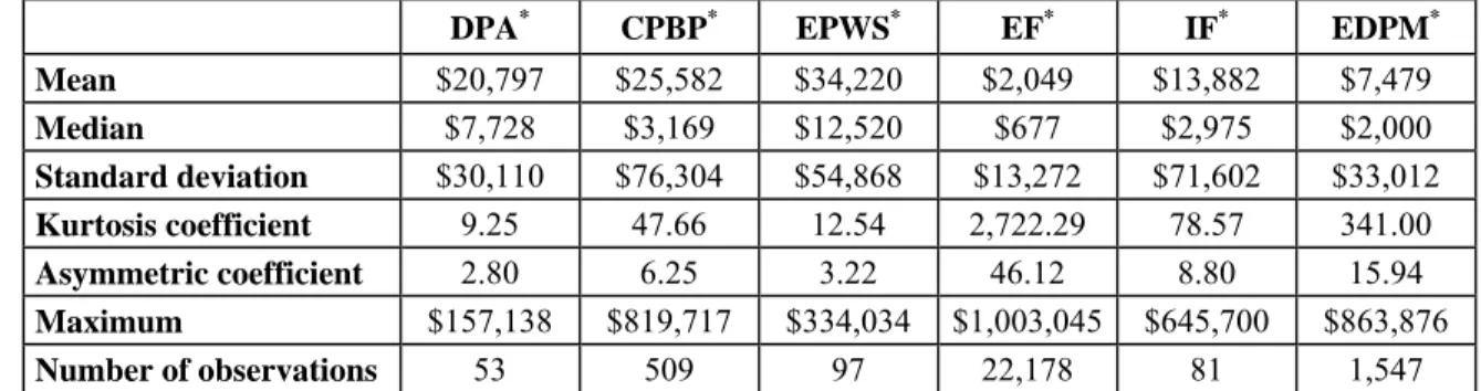
The number of data by type of risk is extremely variable. Table 1a shows that, for the whole bank over the 3-year period, we dispose of only 53 events in the DPA risk category which exceed s, whereas there are 22,178 events involving EF (13,149 of which are below s), mainly linked to card fraud (credit or debit cards).
clients or employees. The mean of losses in EF is on the order of $2,049, if all the data are taken into account. We thus note that EF is a high-frequency and low-severity risk when compared to the type EPWS where the number of losses is only 97 but the mean loss is $34,220. This observation confirms the fact that the amounts of losses by type of risk exhibit different characteristics which justify the distribution by type of risk.
We must admit that the loss data are far from symmetrical in their distribution. A simple comparison between the mean and the median indicates that, in all cases, the median is much lower than the mean, representing a clear indication of asymmetrical distributions. This observation is confirmed by the calculation of the asymmetrical coefficient which is positive in all cases, thus favoring thicker tails. And the very high smoothing coefficients show the existence of leptokurtic distributions with thick tails. We cite the example of the EF type of risk where the smoothing coefficient is on the order of 2,722 and the asymmetry coefficient is evaluated at 46. We in effect note that 98% of the losses are below $10,000.
3.3 Descriptive Statistics on Loss Frequencies
A detailed analysis of the number of daily losses shows us that the frequencies of these losses over the days of the week are not identically distributed. We noted that the frequencies are lower over the weekends. It is possible that there are fewer losses on days when banking institutions are closed. However, it is hard to admit that there should be fewer loss events related to certain types of risk (such as EF…) on weekends than on other days. This result may be due to a bias in the accounting date of the loss. Therefore, one way of getting around this problem is to consider the number of losses by week. This will however mean losing some observations, since we limit our sample to 106 frequencies.
Table 1b presents the descriptive statistics for weekly loss frequencies. We note that the means are lower than the variances, which favors over-dispersion distributions for modeling the frequencies. It is also worth mentioning that we have checked for any end-of-month or end-of-year concentrations which might distort the whole modeling of the frequencies. It is hard to detect any possible end-of-year concentration since we have only a 3-year history. On the other hand, we have noticed a slight
concentration at the end of months for losses of the type, EDPM. The distribution of losses for the other types of risk is uniform over the days and weeks of the month.
The LDA model thus consists in estimating the severity and frequency distributions and determining a certain centile of the distribution of the S (aggregated distribution). The aggregated loss by period is obtained either with a Fourier transformation, as proposed by Klugman et al (2004), or with a Monte Carlo simulation, or by analytical approximation. In what follows, we shall estimate each of the severity and frequency distributions and determine the operational VaR by risk type.
4.
Estimation of the Severity Distribution
The first step in applying the LDA method to calculate capital consists in finding the parametric distributions which offer the best fit for the historical data on loss amounts. The unbiased estimation of the parameters of these distributions will have an enormous influence on the results of operational capital. In this section, we shall explore several methods for estimating the distribution, so that we can achieve a better fit for all the historical data.
The method will, in fact, vary depending on the nature of the data and their characteristics. We begin by estimating the distribution based on all the loss data. However, if the goodness of fit tests we set up rejects these distributions, we must then adopt another method. In this case, it is indeed possible to divide the distribution (especially if the size of the sample permits it) and, consequently, to fit a distribution to each part of the empirical distribution.
Besides considering the behavior of losses and the number of data when choosing the fitting method for severity distributions, the collection threshold for data is also of great importance. In the context of operational risk, most financial institutions have chosen a level at which operational losses will be collected. The fact of using truncated data changes the usual method of estimating parameters. This threshold must thus be taken into account when estimating the parameters.
In the literature, several estimation methods are proposed for estimating parameters. We can cite the maximum likelihood method and the method of moments, among others. However, the latter method
proves harder to use with truncated data, since finding the moments of a truncated distribution is more complicated than estimating the parameters of a distribution whose data are not truncated. It is, however, always possible to estimate the parameters of the distribution of the losses exceeding the collection threshold (Dutta and Perry, 2006). This approach certainly brings us back to the usual estimation of distribution parameters, but it leaves out losses lower than the collection threshold, seeing that the distribution does not take them into account. Thus, we can only generate surplus losses with the distribution chosen. This method poses a problem of underestimation or overestimation of capital, especially if the threshold is high enough and the volume of small losses is appreciable. If this method is used, this bias must be corrected.
Our first step is to identify the distributions which will be tested. We then describe the different estimation methods according to the nature of the data. Finally, we present the results of the estimation for each type of risk and the four distributions tested.
4.1 Distributions Tested
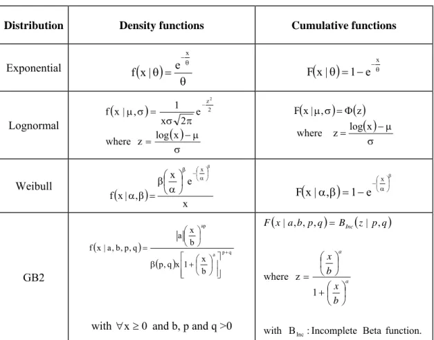
We start by choosing among the various parametric distributions the one which gives the best fit for the loss data. Theoretically, all the continuous distributions with a positive domain of definition are candidates for severity-distribution modeling. Instead of limiting ourselves to a single distribution as do most practitioners in the industry, it is better to start by testing different distributions—simple distributions (with a single parameter) like the exponential; common distributions like the lognormal or the Weibull (with two parameters); and more complex but flexible distributions like the GB2 (with four parameters). We describe the characteristics of each of them and we present their density and cumulative function in the summary table 2
First of all, we test the exponential distribution which offers the advantage of being simple (with just one parameter). Next, the lognormal distribution is tested. This two-parameter distribution is commonly used in practice. And this distribution is, by hypothesis, taken as one which fits loss amounts in several studies (Chernobai, Menn, Truck, and Rachev, 2005b; Frachot, Moudoulaud, and Roncalli, 2003). Both this distribution and the exponential distribution are characterized by moderately thick tails. The
two-parameter Weibull distribution is also tested. Unlike the two preceding distributions, this one has a thin tail. These three distributions thus offer tails of different thickness.
Finally, we also test a family of four-parameter distributions. Though certainly less often used than the others in practice, these distributions do offer a great deal of flexibility. In effect, their four parameters allow them to take numerous forms and to display tails of different thickness.
In specific cases, we also propose the Pareto distribution for estimating the tails. The Pareto can be presented by introducing a -scale parameter. Suppose that Z follows an β α -parameter Pareto distribution, the random variable follows a Pareto distribution with an a shape parameter and a scale parameter β . The f density function and the F cumulative function are respectively the following:
Z X=β α
(
α β)
= αβα+α1 for x ≥β x , , x f ;(
)
⎟ ≥β ⎠ ⎞ ⎜ ⎝ ⎛ β − = β α α or x 1 f x , , x F .4.2 Modeling all the Data
Modeling the amounts of losses will differ according to the data and their characteristics. A first step is to model all the loss data. This involves the types of risk IF and EF for which all the operational loss data are collected. The results of the estimation will be presented only for the risk of IF. The results of the estimation of the parameters related to losses from EF will not be presented, since the goodness of fit tests reject all the distributions tested. We shall thus propose another method for modeling these losses in Section 4.3. Since this model is well known in the literature, it will not be presented here. Given that certain losses related to certain types of risk are truncated whereas others are not, it is important to distinguish between the two estimation models. We develop now the estimation method to be used for truncated data.
To account for the losses not collected, we estimate the conditional parameters only when the losses observed exceed the collection threshold.
Let there be: s: The collection threshold; y: The amounts of losses observed, with y ≥ s; n: The number of losses collected; D: A continuous severity distribution whose parameters are represented by the θ vector.
The density and the cumulative functions of the conditional distribution D arising from the fact that only y is seen to exceed the threshold s are written as follows:
(
)
( )
( )
for y s , s F 1 , y f s y | , y f ≥ θ − θ = ≥ θ ;(
) ( ) ( )
( )
for y s , s F 1 , s F , y F s y | , y F ≥ θ − θ − θ = ≥ θWe have selected to estimate the parameters by optimization of the maximum likelihood method. The optimal solution θMLE solves:
(
)
(
(
)
)
(
1( )
)
1 θ − − θ = θ∑
= , s F nLog , y f Log , y L n i i i (2)Among the losses in our base, we have those related to the following types of risk: DPA; EPWS;
EDPM; and CPBP. The goodness of fit tests that we set up has rejected the fitting of all the distributions
proposed for the last two types previously cited. We shall not present these results. Instead, we shall model them using another method that we develop in the next section.
4.3 Division of the Distribution
In some cases the parametric distributions tested do not fit all the data. This is generally the case when there are very numerous losses or when their empirical distribution has two peaks, etc. In this case, we propose to divide the empirical distribution into parts and to fit the parametric distributions for each part. Several articles in the literature treat the subject of fitting tails of distribution, mainly from the perspective of the theory of extreme values. However, fitting only the tail of the distribution means neglecting the body of the distribution, whereas the latter should play its part in calculating capital and could have a significant impact.
There is no one way to divide a distribution, the important thing being able to find a good fit. The division should go hand in hand with the objective of the fit. In other words, if we make the fitting in order to estimate capital at a 99.9% level, the tails of the distributions will thus come into play. The
quality of the fitting is essential to avoiding an under- or over-estimation of the capital. Thus, in our case, it is important to make an accurate estimation of the tail or the right wing of the distribution of losses.
Once the distribution of the tails has been estimated, the body of the distribution should be estimated. If we fail to obtain a good fit with the distributions tested, we shall divide the body of the distribution into two or more parts. In what follows, we shall present an estimation method for the left, centre, and tail of the distribution.
Modeling with a single parametric distribution did not give conclusive results for the following types of losses: CPBP, EDPM, and EF. Consequently, we opted for dividing the distribution. It should be pointed out that to apply this method it is important to have a sufficiently high number of observations. We must, in effect, have enough data in each part to allow the estimation of the parameters of the distribution. This condition is quite well satisfied for the types of risk to be modeled in this section.
4.3.1 Estimation of the tail of the distribution
In what follows, we plan to model the tails of the empirical distributions. We first choose several sq
loss thresholds corresponding to different high centiles. We next estimate the parameter of the Pareto distribution for each of the loss samples higher than the different sq thresholds. Finally, we select the
threshold for which the Pareto gives the best fit (the distribution for which the p-value of the goodness of fit test is the highest). This method is similar to the one developed by Peters et al (2004).
We have chosen high centiles in order to get a good fitting for the tail. However, it is important to keep enough observations to carry out the estimation. We have decided that at least 50 observations must be kept just for estimating the shape parameter α of the Pareto for each of the risk types.
Let there be: sq: Loss threshold corresponding to the quantity q, this threshold corresponds to the
scale parameter of the generalized Pareto. In effect, we shall each time suppose the scale parameter to be equal to the sq threshold and we estimate only the α parameter; z: Amounts of losses exceeding
the sq threshold; nq: Number of observations z in the sample defined by (zi |zi ≥sq,i=1,2...nq).
(
)
q1 q z s s , , z f α+ α α = α with z≥sq.For the maximum likelihood, the optimal α parameter for the different sq thresholds is :
∑
= ⎟ ⎟ ⎠ ⎞ ⎜ ⎜ ⎝ ⎛ = α q n 1 i q i q MLE s x Log n (3)We have thus estimated the parameter corresponding to each sα q threshold for each of the three
types of risk previously cited. The goodness of fit tests allows us to choose the threshold providing the best fit for the tail.
4.3.2 Estimation of the body of the distribution
Once the tail of the distribution has been modeled, it is then a matter of estimating the distribution which fits the body of the empirical distribution best. Knowing that this latter distribution is represented by all or part of the losses that fall below the centile threshold selected in the preceding section, we shall start with different exponential, lognormal, Weibull and GB2 distributions for the whole sample of losses.
Let there be: sq: Threshold of loss tail selected corresponding to the q centile; : Amounts of
losses falling below the s
' z
q threshold; : Number of observations, being the number of
; D: Distribution to be tested. ' n z' q q i i|z' s ,i 1,2...n ' z < =
The density and the cumulative functions of the distribution D of the losses falling below the tail threshold selected are the following:
(
)
(
( )
)
θ θ = < θ , s F ,' z f s ' z | ,' z f q q ;(
)
(
)
( )
θ θ = < θ , s F ,' z F s ' z | ,' z F q qFor the maximum likelihood, it is a matter of finding the θ parameters which maximize the following function: (4)
(
)
(
(
)
)
(
( )
)
1
θ
−
θ
=
θ
∑
=,
s
F
Log
'
n
,
'
z
f
Log
,
'
z
L
q ' n i i iHowever, as we have already seen, when the loss data are truncated, this must be taken into account in estimating the body of the distribution.
Let there be: s: Collection threshold; sq: Tail threshold selected corresponding to the q centile;
Amounts of losses lower than the sq tail threshold and higher than the collection threshold s; : Number of observations, being the number of
'' z : '' n '' z z''i|s<z''i<sq,i =1 ,2...nq; D: Distribution to be tested.
The density function of the D distribution of the losses between the s threshold and the sq tail
threshold selected is written:
(
θ ≤ <)
=( )
(
θ −θ)
( )
θ , s F , s F ,' ' z f s '' z s | ,' ' z f q q .For the maximum likelihood, parameters maximize the following function: θ
(5)
(
)
[
(
)
]
[
( )
( )
]
1
θ
−
θ
−
θ
=
θ
∑
=,
s
F
,
s
F
Log
'
'
n
,
'
'
z
f
Log
,
'
'
z
L
q '' n i i iThis formula can be used when the data fall between the two thresholds or boundaries. For the risk type CPBP, we have modeled the losses found between the collection threshold and the tail threshold selected. The results of the estimation will be presented in Section 4.4.
As to the types of risk EF and EDPM, modeling the body of the distribution with the parametric distributions proposed proved to be non-conclusive, since the goodness of fit tests failed to select any of them. In this case, we propose a different division of the distribution. We cite the example of the risk type
EF where none of the distributions tested fit the data. A painstaking analysis of the losses from EF do in
fact show that the empirical distribution of the data have two peaks, the second of which stands at the level of $5,000. We thus divide the distribution at the level of this point. We estimate the left wing of the distribution using the maximum likelihood method shown in equation (4). Seeing that the losses are contained between the two thresholds, the centre of the empirical distribution is estimated using another parametric distribution based on function (5) of the maximum likelihood.
As to the risk type EDPM, estimation of the left wing and the centre of the empirical distribution is done with the likelihood function (5), since the data are truncated at the collection threshold.
We set up the Kolmogorov-Smirnov (KS), Anderson Darling (AD), and Cramér-von-Mises (CvM) tests along with the parametric bootstrap procedure. The Appendix A2.1 presents the algorithm for the KS parametric bootstrap procedure. It should be noted that, when applying the test, we must take the characteristics of the sample into account. In other terms, if the data are truncated or contained between two thresholds, a sample respecting the same condition must be generated in the parametric-bootstrap procedure before calculating the statistic.
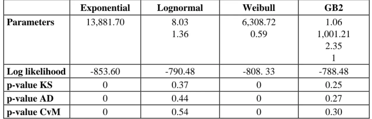
4.4 Results from Estimation of the Parameters
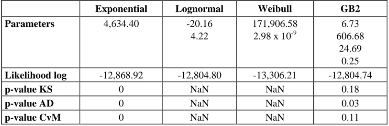
Table A1 presents the results obtained from estimating the distributions for the risk types IF, DPA, and EPWS. Unlike the other types of risk with truncated losses, losses connected with the IF risk are integral. The results of this type of risk synthesized in Table A1a show that the lognormal and GB2 distributions fit the loss data well, whereas the fitting of the exponential and Weibull distributions are rejected. However, the lognormal distribution has a higher p-value than that of the GB2. We thus retain the lognormal distribution as the severity distribution which best describes the behavior of incidents of IF in the bank studied.
Tables A1b and A1c present the results for the risk types: DPA, and EPWS. Remember that these losses are truncated at the s level. Only the lognormal and GB2 distributions offer a good fit for the truncated-losses data. The KS, AD, and CvM tests for the Weibull distribution could not be carried out for the two types of risk. Accounting for the truncature when modeling losses does, in fact, greatly complicate the estimation of distributions and standard tests could not be applied. For the types of risk DPA, and
EPWS, we note that the results of the goodness of fit tests are similar for the lognormal and GB2
distributions. In what follows, we opt for the lognormal, as it is simpler than the GB2.
As for the other types of risk, we divide the empirical distribution, since none of the distributions can be retained with the first method. Moreover, since the number of observations is rather high for the
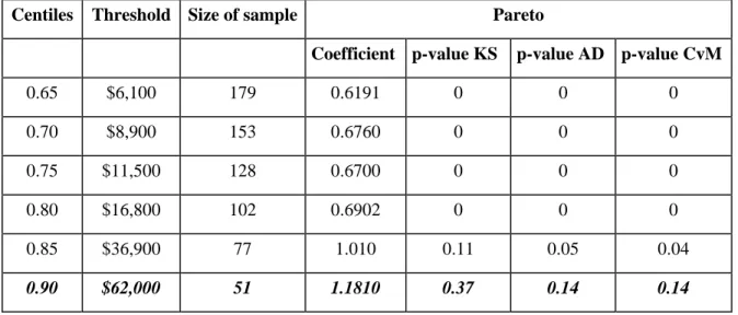
three samples, the division is possible, as is described in the preceding section. For the type of risk CPBP, we first estimate the tail of the distribution by testing the Pareto distribution on several samples of the tail corresponding to high centiles. The results in Table A2a allow us to retain the threshold of $62,000. In other words, losses above this threshold follow a 1.8 Pareto parameter. The losses below this threshold have been modeled by the four distributions cited in Section 4.1. The results of the goodness of fit tests (Table A2b) reject all the distributions except the GB2. We thus retain this distribution for modeling losses situated below the $62,000 threshold.
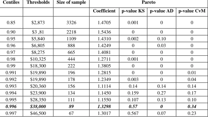
We also begin by modeling the tail in the case of the risk type EDPM. Several thresholds corresponding to different centiles are chosen. Based on the three tests, the best fit of the Pareto is obtained for the $26,000 threshold corresponding to the 96% centile (Table A3). The parameter of the Pareto is estimated at 1.11. We next estimate the body of the distribution with the distributions proposed. None of the distributions fit the empirical data below the tail threshold. We have consequently divided the body of the distribution into two parts forming the left wing and the center of the distribution. The results in Table A3b, obtained from estimating the left wing (data contained between s and s’) of the distribution, show that only the GB2 offers a good fit for the historical data according to the p-value of the KS test. It should be mentioned that the estimation of the lognormal and Weibull distributions do not give coherent parameters. This fails to establish the KS, AD, and CvM tests. As for the centre of the distribution, we model the losses with the same distributions. The results from the goodness of fit test show that the lognormal and GB2 distributions offer a good fit. The comparison of the p-values of the two distributions favors the GB2 model (Table A3c).
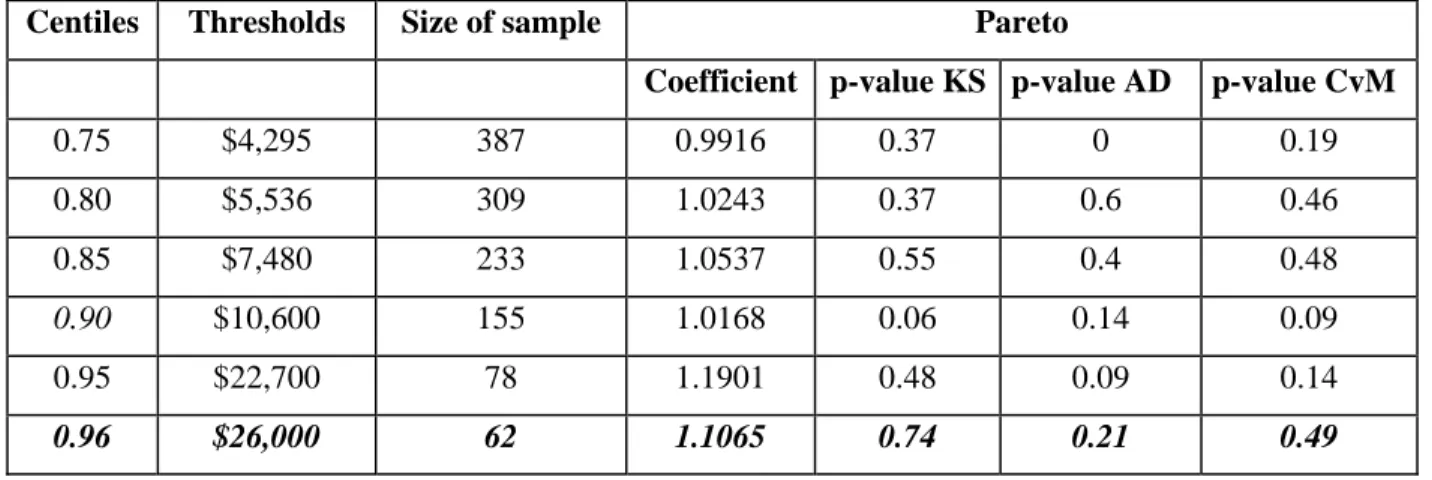
The same method is applied to the EF risk type. To estimate the tail, we test several thresholds corresponding to numerous centiles (between 0.85 and 0.997), since the tail of the sample allows us to do so (22, 179). We retain the threshold of $38,000 and the parameter of the Pareto is estimated at 1.33. We next divide the body of the empirical distribution, since attempts to find a fit for all the data below the tail threshold fail to produce conclusive results. We thus estimate the left wing of the distribution composed of
reject the fit for the other distributions. Finally the centre of the empirical distribution is also modeled with a GB2 distribution.
We should point out that, in each case, the exponential and Weibull distributions fail to offer a good fit for the data. In most cases, the GB2 distribution turns out to be the best candidate for modeling the amounts of operational losses. This confirms our initial hypothesis stipulating that, given its great flexibility, the GB2 would offer a good fit for the data. But we also note that estimating this distribution, especially for truncated data, is rather difficult.
5.
Estimation of the Frequency Distribution
5.1 Distributions Tested
We propose the Poisson and negative binomial distributions for estimating the number of operational losses. Several studies have already used the Poisson to model operational losses, whereas few have used the negative binomial for this purpose.
Let Y be a discrete positive random variable:
( )
λ Poisson ~ Y then(
)
! y e y Y P i y i i λ = = −λ( )
α,β negative Binomial ~ Y then(
) (
)
( )
α ⎟⎟ ⎠ ⎞ ⎜⎜ ⎝ ⎛ β + × ⎟⎟ ⎠ ⎞ ⎜⎜ ⎝ ⎛ β + β × α Γ + α Γ = = 1 1 1 ! y y y Y P i y i i i5.2 Estimation of the Parameters
For each of the six types of risk, we estimate the parameters of each of the two distributions using maximum likelihood. As we have already pointed out, we model both daily and weekly frequencies in order to correct any possible collection bias.
Remember that, for certain types of risk (DPA, EPWS, CPBP and EDPM), the losses are collected only at a specific threshold. We have taken this truncature threshold into account in estimating the severity distribution. The same modeling has to be done for the frequencies. Note that these are not truncated frequency distributions. We in fact have at our disposal the number of losses above the collection
threshold. The parameters estimated must be corrected to account for the number of losses below the truncature threshold.
5.3 Correction of the Parameters
For the Poisson distribution, Frachot et al (2003) have already proposed correcting the parameter in order to account for the number of uncollected operational losses. We extend the case where the
λ
λ parameter is random.
Let there be: :The number of losses collected, : The number of real losses, X: The amount of the losses, s: The collection threshold, F: Cumulative function of the severity distribution, with:
;
obs
y
y
real( )
s Pr[
X s]
F = ≤
Suppose that the frequency distribution of all the losses is random parameter Poisson . In what follows, we shall determine the distribution of the frequencies observed. The probability of observing i operational losses amounting to more than s is (Dahen, 2007):
real λ
(
)
( )
F( )s j j real j i estimated obs real estimated e ! j s F ! i e E i y P λ ∞ = λ − λ = ⎪⎭ ⎪ ⎬ ⎫ ⎪⎩ ⎪ ⎨ ⎧ λ = =∑
0 withwhere λestimated =λF
( )
s with F( )
s =1−F( )
s (6) In the case where λ~Γ( )
α,β which corresponds to the case where⎟⎟ ⎠ ⎞ ⎜⎜ ⎝ ⎛ β + α 1 1 , binomial negative ~
Y , the parameters estimated based on the data observed are
( )
(
, Fs)
~
estimated Γαβ
λ . The number of losses collected thus follows a negative-binomial distribution of parameters
( )
⎟⎟⎠⎞ ⎜⎜ ⎝ ⎛ β + α s F 1 1, . Thus, once the parameters of the negative binomial have been estimated, we correct these parameters to account for the unobserved frequencies of the losses below the collection threshold. The real parameters
(
αreal,δreal)
are thus:estimated real
=
α
α
and
( )
( )
s
F
s
F
estimated estimated real−
δ
δ
=
δ
1
(7)
Where
the parameter is defined such that
δ β + = δ 1 1.
At this stage, it is important to test the degree of fitting of the distributions estimated for the different periods chosen (daily and weekly) and for each of the types of risk. As we are dealing with discrete data, we cannot apply the same tests used earlier to test the severity distributions. We thus set up in the Appendix A2.2 a test with parametric bootstrap, constructed in the same way as the Kolmogorov-Smirnov test.
2
χ
5.5 Results of the parameters’ estimation
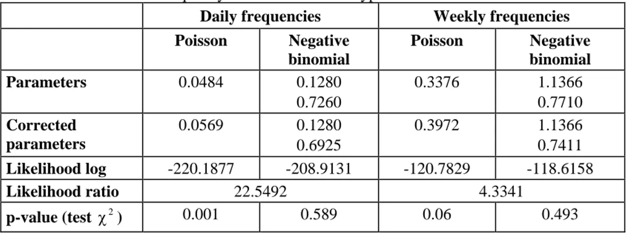
Table A5 presents the results of the estimation of the Poisson and negative-binomial distributions for each of the six types of risk. It is worth noting that in all the cases, the Poisson distribution is rejected by the test. This confirms our expectations since the data present an over-dispersion that must be modeled by another distribution. This fact calls into question all the studies on the calculation of operational capital which use the Poisson model to estimate loss frequencies. The negative-binomial distribution offers a good fit for the daily or weekly loss numbers.
2
χ
Concerning the frequency period, we note that for the types of risk EF, IF, and EDPM (Tables A5a, A5b, A5f) the modeling works better when weekly frequencies are chosen. This fits in with our initial analysis showing a potential bias in accounting for certain losses. For the other types of risk, we retain the daily frequencies, as based on the values of the p-values of the χ2 test (Tables A5c, A5d, A5e).
On the other hand the likelihood ratio test is higher than χ2
(
5%,1)
in all the cases. This result shows that we reject the null hypothesis stipulating that the over-dispersion coefficient is null. This fact confirms the previous results confirming rejection of the Poisson model. We thus retain the negative binomial model as the one with the best fit for the frequency data. We have also corrected the parameters to account for the loss numbers falling below the threshold for all the risk types except EF and IF. It should be mentioned that, based on the expertise and judgment of the directors of the bank studied, we fix F(s) exogenously.6.
Calculation of Operational VaR by Type of Risk
6.1 Aggregation of the Distributions with the Internal Data
Remember that our objective is to estimate the annual value at risk at a 99.9% confidence level, as recommended by the regulatory authorities. We start by first determining the distribution which models the severity of operational risks by event for each of the risk types. The second step consists in determining the distribution which best fits the frequency data. At this stage of the analysis, it is suitable to aggregate the two distributions to obtain the aggregated distribution of the annual losses. Several aggregation methods, which we have already described, are available in the literature. We choose the Monte Carlo simulation method to derive the non-parametric distribution of the annual losses. This method is not the quickest but it has the advantage of being very precise. We apply the method already described by Cruz (2002) in the context of operational risk.
6.2 Comparison of our Model with the Standard Model
We define the standard model as being the simple method frequently found in the literature and obtained based on the lognormal and the Poisson distributions. Moreover, no consideration is given to missing losses. We have chosen this model because it is frequently used in practice and has been the subject of several research studies. We shall thus test this model’s robustness compared to that of the model we have developed. We expect to find that poor specification of the distributions and their failure to fit all the data will bias the calculation of the capital required.
We have also chosen only three types of risk to do this analysis: IF, EPWS and EF. These types of risk will allow us to compare our model to the standard model. In table A6, we present the results of the non-conditional estimation of the lognormal distribution. We also present the results obtained from modeling the number of weekly losses with the Poisson distribution. Since the standard model is used, no goodness of fit test is done.
Table 3 compares the variation percentages for the mean of annual losses and the VaR (confidence levels at 90; 95; 99 and 99.9%) obtained with the standard model to those obtained with the model
developed in this study. We note that the results are very different in most of the cases. The standard model underestimates enormously the annual mean of losses and the VaR.
For the type of risk IF, the data are not truncated and the severity distribution is the same in both models. Thus, the difference in the results of the two models measures the impact of the poorly specified frequency distribution for this type of risk. The mean of annual losses are almost equal, whereas a difference of as much as 2% is noted between the VaR of the two models.
For the risk type EPWS, the data are truncated and the severity distribution is the same in both models. Thus, the difference in the results obtained by the two models measures the impact of the poorly specified frequency distribution and the failure to consider the truncature threshold for this type of risk. Thus, the underestimation of the mean of annual losses (-5%) and of the VaR (-27%) shows the importance of choosing the proper frequency distribution and of considering the data below the threshold.
As to the type of risk EF, the severity and frequency distributions are not the same in the two models. The results will thus measure the impact of the poor choice of distributions on the mean of annual losses and on the VaR. In effect, the 99.9% VaR calculated with the standard model is underestimated (by 82%) compared with the one calculated using our model. This confirms our expectations. It is important to choose distributions that fit the loss data well, in order to determine the level of capital reflecting a bank’s true exposure to operational risk.
We also note that the underestimation is larger when the VaR confidence level is high. Indeed, for the type of risk EF, there is only a minimal difference in the means for annual losses between the two models, whereas this difference is on the order of 6% between the 90% VaRs and goes as high as 82% between the 99.9% VaRs. This thus shows that the standard model underestimates the thickness of the tail of the aggregated distribution.
So this analysis shows that the poorly specified severity and frequency distributions result in serious biases in the calculation of capital. The VaR calculated with the standard model does not reflect at all the bank’s real exposure. Moreover, failure to consider the uncollected losses leads to an inaccurate and
biased estimation of capital. Our method is thus a good alternative to the standard model, since it allows an accurate description of the tails of the severity distributions without ignoring the body.
6.3 Combination of Internal and External Data
The current context of operational risk imposes the use of external data for calculating the value at risk. Indeed, the losses collected do not reflect the bank’s real exposure, since certain less frequent, but potentially heavy losses are not necessarily captured in the internal data base. They can, nonetheless, have a serious influence on operational risk capital. This is mainly explained by the fact that the history of losses is short and the collection is not yet exhaustive. All these factors argue in favor of combining internal and external losses. External losses will be scaled by applying the same method used in Dahen and Dionne (2007).
Concerning the severity distribution describing the behavior of external losses scaled to the Canadian bank studied, we shall take the split GB2 model estimated in the Dahen study (2007). On the other hand, the Dahen and Dionne study (2007) shows how it is possible to determine parameters of the frequency distribution which make it possible to scale and fit the data. We shall thus retain the negative-binomial model with a regression component.
From the theorem of Larsen and Marx (2001), we find that, if frequency losses of more than $1 M are independent and identically distributed according to a negative-binomial model, then the parameters of the annual negative-binomial distribution are ⎟
⎠ ⎞ ⎜ ⎝ ⎛ p , 11 ri
with
( )
ri,p the negative-binomial parameters determined based on the Dahen and Dionne study (2007) for modeling the number of losses on an 11-year horizon.Knowing the severity and frequency distribution, we shall aggregate them in the same way that we did for the internal data. We set up an algorithm in Appendix 3 which makes it possible to aggregate the internal and external data with a view to determining the empirical distribution of the annual losses and to calculating their 99.9th percentile.
6.4 Determination of the VaR
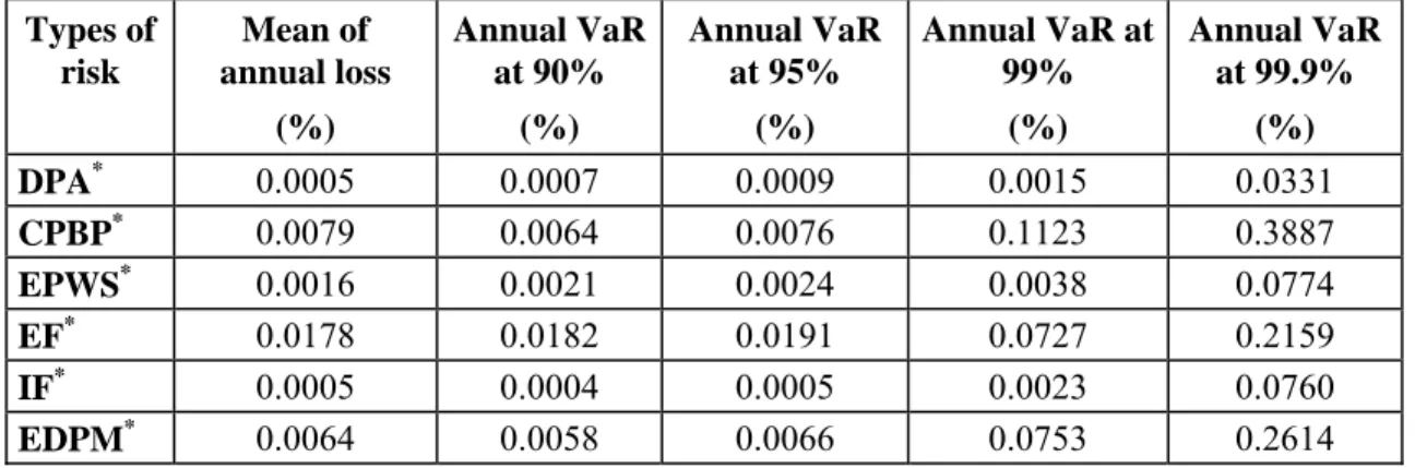
Table 4 presents the results of the mean of annual losses and the VaR calculated at the 95%, 99%, and 99.9% confidence level. These results take into account the internal losses collected within the bank as well as the external losses scaled to the financial institution under study. Out of respect for the confidentiality of the information from the bank studied, the results are presented as a percentage of the total assets of that bank in 2004. We present the results by type of risk and we show that the type of risk,
CPBP presents the greatest operational value at risk. This confirms the result found by Dutta and Perry
(2006) in their study based on data from 7 banks. The types of risk EF and EDPM come respectively in second and third position in terms of their VaR scope. The type of risk which presents the least risk is
DPA. It is worth noting that this classification of types of risk is not respected when we observe the values
of the mean of annual losses.
6.5 Impact of the Combination of Internal and External Data on the Results
To highlight the impact of integrating external data in the calculation of the VaR, we consider three types of risk: DPA; EPWS and IF. We have chosen these types of risk because the internal base shows no extreme losses of over one million dollars for them. Thus, a comparison between the VaRs calculated with only internal data and those calculated based on the combination of internal and external data will show us the importance of external data for filling in the tails of the distributions.
We calculate the mean of annual losses as well as the VaR of different centiles based on a first sample composed only of internal loss data, whereas the second sample incorporates external loss data for the three types of risk cited above. The results presented in table 5 show that the VaR is greatly underestimated when based solely on internal data. The underestimation reaches 99% for the type of risk
IF (VaR at 99.9%). In effect, the losses linked to this type of risk can be too high, like the losses sustained
by the Allied Irish Bank and Barings as the result of unauthorized transactions. Remember that no extreme events have occurred in the history of these three types of risk. Including the possibility of events of more
than one million dollars will make it possible to give a better description of the tails of the aggregated distributions and thus to reflect the level of unexpected losses.
7.
Conclusion
The objective of this article is to construct a robust method for measuring operational capital. We have thus presented a method which consists in carefully choosing the right severity distribution, by making sure to take uncollected losses into account. The results have shown that in most cases the GB2 distribution provides a good fit for all the data or for the body of the empirical distributions. The GB2 thus proves to be a good candidate for consideration when determining the severity distribution of operational losses. As the GB2 has already been applied recently in several financial domains, this article argues in favor of the relevance of its application in modeling operational risk. As to the tails of the distributions, we have chosen the Pareto distribution.We have also tested the Poisson and negative-binomial distributions for modeling the frequencies of losses. We have shown that, unlike the negative-binomial model, the Poisson model is retained in none of the cases. In order to take into account the number of losses falling below the collection threshold, a correction was made in the parameters estimated.
In order to show the robustness of our model, we have compared it to the standard model constructed on the most commonly used distributions (lognormal and Poisson), but without considering the truncature threshold. The results have shown that the standard model greatly underestimates the operational value at risk.
We have also set up an algorithm in order to combine the internal and external losses scaled to the Canadian bank studied. The results of the VaR reflect the reality more adequately, since the internal data do not include losses of a very large scope. Moreover, an analysis of the impact of the integration of external data on the VaR has revealed that it is largely underestimated when the calculations are based solely on internal data. This proves the importance of combining internal and external data in calculating a bank’s unexpected losses.
So this mode, as developed and applied to real data from a Canadian bank, can be implemented in any financial institution. However, note that there needs to be a sufficient number of data for a parametric modeling of distributions. We have fixed this number in an arbitrary fashion, since it is not the subject of this contribution. A statistical study making it possible to determine the minimal number required for modeling distributions would thus justify our choice.
Remember that we have calculated the unexpected loss for only six types of risk. For the seventh type of risk Business Disruption and System Failures, the number of observations is limited, which prevents us from estimating the loss with the LDA method. We thus think that other methods based on qualitative factors can be applied, methods like scenario analysis (Scandizzo, 2006). It would be interesting to see how this method could be implemented in practice. It would also be interesting to calculate the aggregated capital of the whole bank. Taking into consideration the dependence between types of risk makes it possible to find the exact value of the aggregated capital. The copula theory can be used for this and can thus be an interesting avenue of research (Frachot, Roncalli, and Salomon, 2004 and Chavez-Demoulin, Embrechts, and Nešlehová, 2006).
Besides, the case study done in this article can be used as a business case. If we dispose of the operational-risk capital allotted to all types of risk including the risk type Business Disruption and System
Failures, it will be possible to use the copula theory to calculate the aggregated capital at the level of the
bank. We can consequently compare the capital found with the advanced method to the capital calculated with the standardized or basic method. It is expected that the capital estimated with the advanced method will be lower than that found with other methods, when the true dependence between the types of risk is carefully evaluated.
Bibliography
Alexander, C. (2003), Operational Risk: Regulation, Analysis and Management, FT Prentice Hall: London.
Artzner, P., F. Delbaen, J. M. Eber and D. Heath (1999), “Coherent Measures of Risk,”
Baud, N., A. Frachot and T. Roncalli (2002), “How to Avoid Over-estimating Capital Charge for Operational Risk?” Working Paper, Groupe de Recherche Opérationnelle, Crédit Lyonnais, France.
Bee, M. (2006), “Estimating the Parameters in the Loss Distribution Approach: How Can We Deal with Truncated Data?” In The Advanced Measurement Approach to Operational Risk, edited by E. Davis, Risk Books: London.
Böcker and Klüppelberg (2005), “Operational VaR: a Closed-Form Approximation,” Risk
Magazine, December 2005, 90-93.
Chapelle, A., Y. Crama, G. Hübner and JP. Peters (2004), “Basel II and Operational Risk: Implications for Risk Measurement and Management in the Financial Sector,” Working Paper 51, National Bank of Belgium.
Chavez-Demoulin, V., P. Embrechts and J. Nešlehová (2006) “Quantitative Models for Operational Risk: Extremes, Dependence and Aggregation,” Journal of Banking and Finance, 30, 10, 2635-2658.
Chernobai, A., C. Menn, S. T. Rachev and C. Trûck (2005c) “Estimation of Operational Value-at-Risk in the Presence of Minimum Collection Thresholds.” Technical Report, University of California Santa Barbara.
Chernobai, A., C. Menn, S. T. Rachev, C. Trûck and M. Moscadelli (2006) “Treatment of Incomplete Data in the Field of Operational Risk: The Effects on Parameter Estimates, EL and UL Figures,” The Advanced Measurement Approach to Operational Risk, edited by E. Davis, Risk Books: London.
Chernobai, A., C. Menn, S. Trûck and S. T. Rachev (2005a) “A Note on the Estimation of the Frequency and Severity Distribution of Operational Losses,” Mathematical Scientist 30, 2, 87-97.
Chernobai, A. and S. Rachev (2006) “Applying Robust Methods to Operational risk Modeling,”
Journal of Operational Risk 1, 1, 27-41.
Chernobai, A., S. Rachev and F. Fabozzi (2005b) “Composite Goodness-of-Fit Tests for Left-Truncated Loss Samples,” Technical Report, University of California Santa Barbara.
Cruz, M. G. (2002) Modeling, Measuring and Hedging Operational Risk, John Wiley & Sons, LTD: Chichester.
Cummins, J. D. and L. R. Freifelder (1978) “A Comparative Analysis of Alternative Maximum Probable Yearly Aggregate Loss Estimators,” The Journal of Risk and Insurance, 45, 1, 27-52.
Dahen, H. (2007) “ La Quantification du Risque Opérationnel des Institutions Bancaires,” Ph.D thesis, HEC Montreal.
Dahen, H. and G. Dionne (2007) “Scaling Models for the Severity and Frequency of External Operational Loss Data,” Working paper 07-01, Canada Research Chair in Risk Management.
de Fontnouvelle, P., V. DeJesus-Rueff, J. Jordan and E. Rosengren (2003) “Capital and Risk : New Evidence on Implications of Large Operational Losses,” Working Paper, Federal Reserve Bank of Boston. de Fontnouvelle, P., J. Jordan and E. Rosengren (2004) “Implications of Alternative Operational Risk Modelling Techniques,” Working Paper, Federal Reserve Bank of Boston.
Dutta, K. and J. Perry (2006), “A Tale of Tails: An Empirical Analysis of Loss Distribution Models for Estimating Operational Risk Capital.” Working Paper 06-13, Federal Reserve of Boston.
Ebnother, S., P. Vanini, A. McNeil and P. Antolinez-Fehr (2001) “Modelling Operational Risk.” Working Paper.
Embrechts, P., H. Furrer and R. Kaufmann (2003) “Quantifying Regulatory Capital for Operational Risk,” Derivatives Use, Trading and Regulation, 9, 3, 217-233.
Embrechts, P., C. Klüppelberg and T. Mikosch (1997) Modelling Extremal Events for Insurance
and Finance, Springer Verlag: Berlin.
Frachot, A., O. Moudoulaud and T. Roncalli (2003). “Loss Distribution Approach in Practice,” in
The Basel Handbook: A Guide for Financial Practioners, edited by Micheal Ong: Risk Books, 2004.
Frachot, A., T. Roncalli and E. Salomon (2004) “The Correlation Problem in Operational Risk,”
Groupe de Recherche Opérationnelle, Crédit Lyonnais, France.
Klugman, S. A, H. H. Panjer and G. E. Willmot (1998) Loss Models, From Data to Decisions, Wiley Series in Probability and Statistics: New York.
Larsen, R. J. and M. L. Marx (2001) An Introduction to Mathematical Statistics and its
Applications, 3ème édition, Prentice Hall.
Moscadelli, M. (2004) “The Modelling of Operational Risk: Experience With the Analysis of the Data Collected by the Basel Committee.” Working Paper, Banca d’Italia, Italie.
Peters, J. P., Y. Crama and G. Hübner (2004) “An Algorithmic Approach for the Identification of Extreme Operational Losses Threshold.” Working Paper, Université de Liège, Belgique.
Scandizzo, S. (2006) “Scenario Analysis in Operational Risk Management,” in The
Table 1: Descriptive Statistics
We present descriptive statistics for the amounts and frequencies of operational losses of a Canadian bank over the period running from 1/11/2001 to 31/10/2004
Table 1a: This table presents the descriptive statistics for loss amounts by event and type of risk over a
3-year period.
DPA* CPBP* EPWS* EF* IF* EDPM*
Mean $20,797 $25,582 $34,220 $2,049 $13,882 $7,479 Median $7,728 $3,169 $12,520 $677 $2,975 $2,000 Standard deviation $30,110 $76,304 $54,868 $13,272 $71,602 $33,012 Kurtosis coefficient 9.25 47.66 12.54 2,722.29 78.57 341.00 Asymmetric coefficient 2.80 6.25 3.22 46.12 8.80 15.94 Maximum $157,138 $819,717 $334,034 $1,003,045 $645,700 $863,876 Number of observations 53 509 97 22,178 81 1,547
* DPA: Damage to Physical Assets / CPBP: Clients, Products and Business Practices / EPWS: Employment,
Practices, and Workplace Safety / EF: External Fraud/ IF: Internal Fraud / EDPM: Execution, Delivery and Process Management
Table 1b: This table presents daily and weekly frequencies by risk type, over 3-year period.
Daily loss frequencies by type of risk, over a 3-year period
DPA* CPBP* EPWS* EF* IF* EDPM*
Mean 0.0484 0.4644 0.0885 20.2354 0.0739 1.4115 Median 0 0 0 18 0 1 Mode 0 0 0 0 0 0 Variance 0.0643 1.0617 0.1209 369.7491 0.1069 9.3693 Minimum 0 0 0 0 0 0 Maximum 3 14 4 226 4 66
Weekly loss frequencies by type of risk, over a 3-year period.
Mean 0.3376 3.2420 0.6178 141.2611 0.5159 9.8535 Median 0 2 0 148 0 8 Mode 0 2 0 125 0 4 Variance 0.4302 10.3513 0.8530 2689.7070 0.7513 87.8566 Minimum 0 0 0 50 0 0 Maximum 3 17 4 447 4 80
* DPA: Damage to Physical Assets / CPBP: Clients, Products and Business Practices / EPWS: Employment,
Practices, and Workplace Safety / EF: External Fraud/ IF: Internal Fraud / EDPM: Execution, Delivery and Process Management
Table 2: Distributions Studied
Distribution Density functions Cumulative functions
Exponential
( )
θ = θ θ −x e | x f(
θ)
= − −θ x e 1 | x F Lognormal(
)
( )
σ μ − = π σ = σ μ − x log z where e 2 x 1 , | x f 2 z2(
)
( )
( )
σ μ − = Φ = σ μ x log z where z , | x F Weibull(
)
x e x , | x f x⎟β ⎠ ⎞ ⎜ ⎝ ⎛ α − β ⎟ ⎠ ⎞ ⎜ ⎝ ⎛ α β = β α(
)
β ⎟ ⎠ ⎞ ⎜ ⎝ ⎛ α − − = β α x e 1 , | x F ( ) ( ) a p q ap b x 1 x q , p b x a q , p , b , a | x f + ⎥ ⎥ ⎦ ⎤ ⎢ ⎢ ⎣ ⎡ ⎟ ⎠ ⎞ ⎜ ⎝ ⎛ + β ⎟ ⎠ ⎞ ⎜ ⎝ ⎛ =with ∀x≥0 and b, p and q >0
(
)
(
)
function. Beta Incomplete : B with 1 z where , | , , , | Inc a a Inc b x b x q p z B q p b a x F ⎟ ⎠ ⎞ ⎜ ⎝ ⎛ + ⎟ ⎠ ⎞ ⎜ ⎝ ⎛ = = GB2Table 3: Comparison between Our Model and the Standard Model
We compare the mean of annual losses (excluding external losses) as well as the annual VaR, at the 90; 95; 99 and 99,9% level of confidence, as calculated based on the standard model and the one we have set up in this article for the types of risk Internal Fraud, Employment, Practices, and Workplace Safety, and External Fraud We present the variation in percentage of the results obtained with the standard model compared to the results from our model.
Variation of the standard model compared to our model (%) Types of risk Variation of losses /year Variation of annual VaRs at 90% Variation of annual VaRs at 95% Variation of annual VaRs at 99% Variation of annual VaRs at 99.9% IF* -0.06 -2.06 -2.18 -1.68 -1.34 EPWS * -4.67 -9.40 -11.89 -17.07 -27.32 EF* 0.95 -5.62 -13.50 -40.28 -81.59
Table 4: Operational VaR by Type of Risk
We present the results of the estimation of the mean of annual losses and annual values at risk at the 90%, 95%, 99% and 99,9% confidence level by type of risk. These results are derived from the combination of scaled internal and external data. The results are presented as a percentage of the total 2004 assets of the bank studied. Types of risk Mean of annual loss (%) Annual VaR at 90% (%) Annual VaR at 95% (%) Annual VaR at 99% (%) Annual VaR at 99.9% (%) DPA* 0.0005 0.0007 0.0009 0.0015 0.0331 CPBP* 0.0079 0.0064 0.0076 0.1123 0.3887 EPWS* 0.0016 0.0021 0.0024 0.0038 0.0774 EF* 0.0178 0.0182 0.0191 0.0727 0.2159 IF* 0.0005 0.0004 0.0005 0.0023 0.0760 EDPM* 0.0064 0.0058 0.0066 0.0753 0.2614
*DPA: Damage to Physical Assets / CPBP: Clients, products and Business Practices / EPWS:
Employment, Practices, and Workplace Safety / EF: External Fraud / IF: Internal Fraud / EDPM: Execution, Delivery and Process Management
Table 5: Impact of the Integration of External Data on the VaR
We present the results of the comparison between the mean of annual losses and the annual values at risk at the 90%, 95%, 99%, and 99.9% confidence level calculated based on internal data to those calculated based on internal and external loss data.
Variation of the model with internal data compared to the model with internal and external data (%)
Types of risk Mean of annual losses (%) Annual VaR at 90% (%) Annual VaR at 95% (%) Annual VaR at 99% (%) Annual VaR at 99.9% (%) DPA* -11.83% 1.46% 3.11% 15.24% -88.73% EPWS* -18.42% 0.67% 3.68% -1.08% -91.26% IF* -57.30% -5.31% -8.98% -72.29% -98.63% *DPA: Damage to Physical Assets / EPWS: Employment, Practices, and Workplace Safety / IF: Internal