2019 — Design of photovoltaic energy systems for isolated communities

DESIGN OF PHOTOVOLTAIC ENERGY SYSTEMS FOR

ISOLATED COMMUNITIES

by

Abdoulaye SOW

MANUSCRIPT BASED THESIS

PRESENTED TO ÉCOLE DE TECHNOLOGIE SUPÉRIEURE IN PARTIAL

FULFILLMENT FOR THE DEGREE OF MASTER IN MECHANICAL

ENGINEERING

M.A.SC

MONTREAL, NOVEMBER 08 TH ₂₀₁₉

ÉCOLE DE TECHNOLOGIE SUPÉRIEURE UNIVERSITÉ DU QUÉBEC

© Copyright reserved

It is forbidden to reproduce, save or share the content of this document either in whole or in parts. The reader who wishes to print or save this document on any media must first get the permission of the author.

BOARD OF EXAMINERS THIS THESIS HAS BEEN EVALUATED BY THE FOLLOWING BOARD OF EXAMINERS

Mr. Daniel Rousse Thesis Supervisor

Professor, Mechanical engineering at École de technologie supérieure

Mr. Mathias Glaus, President of the Board of Examiners

Professor, Construction engineering at École de technologie supérieure

Didier Haillot, Member of the jury

Invited Professor, Mechanical engineering at École de technologie supérieure

THIS THESIS WAS PRENSENTED AND DEFENDED

IN THE PRESENCE OF A BOARD OF EXAMINERS AND PUBLIC JULY 18TH ₂₀₁₈

ACKNOWLEDGMENT

I would first like to thank my thesis advisor Mr Daniel Rousse Professor in Mechanical engineering at École de technologie supérieure for his patience, motivation, and support. He consistently allowed this paper to be my own work but steered me in the right direction whenever he thought I needed it.

I would also like to thank the member of the t3e research group for the stimulating discussions, and for all the fun we have had in the last two years.

I would also like to acknowledge the financial support for conducting this research from FRQNT (Fonds de Recherche du Québec Nature et Technologies), MERN (Ministère de l’Énergie et des Ressources Naturelles du Québec) and from M. Michel Trottier for his generous donation to the t3e research group

Finally, I must express my very profound gratitude to my parents Ousmane and Sophie for providing me with unfailing support and continuous encouragement throughout my years of study and through the process of researching and writing this thesis. I also want to thank my brothers Thierno and Mouhamed and my sister Oumouratou for continuing motivating me and supporting me. This accomplishment would not have been possible without my family. Thank you.

CONCEPTION D’UN SYSTÈME D’APPROVISIONNEMENT ÉNERGETIQUE PHOTOVOLTAIQUE POUR COMMUNAUTÉS ISOLÉES

Abdoulaye SOW

RÉSUMÉ

L'accès à l'énergie joue un rôle important dans un processus de développement économique social et humain. Cependant, de nos jours 1,3 milliard de personnes n'ont toujours pas accès à l'électricité. La majorité de ces communautés vivent dans les zones rurales des pays sous-développés. Pour faire face à cette question, les systèmes PV décentralisés constituent des solutions appropriées pour l'électrification et le pompage de l'eau. De plus, avec la récente baisse des coûts des panneaux photovoltaïques et des batteries, des systèmes plus sophistiqués intégrant le contrôle de l’énergie produite en fonction du niveau de consommation ont été développés.

Pour soutenir cette implantation, des logiciels et outils numériques permettant un dimensionnement précis et optimal de ces systèmes ont été développés. PV SOL, PV SYST, HOMER ou iHOGA peuvent être cités comme exemples de logiciels de prédiction. Néanmoins, malgré le niveau de sophistication de ces programmes, il existe un besoin de proposer un logiciel de prédiction simple, évolutif, précis et gratuit pour permettre aux communautés isolées de calculer les systèmes dont elles ont besoin.

Ce mémoire présente un programme qui utilise un algorithme génétique pour le dimensionnement optimal d’un système PV-batteries pour électrifier les communautés hors-réseau. Le programme a été développé en Python. Il simule le comportement des systèmes PV-batteries installés dans tous les endroits où des données météorologiques sont disponibles. En outre, une banque de données modifiable, adaptable et évolutive avec le temps des différents composants du système est disponible.

Dans ce mémoire, une maison, une école, des lampadaires et un centre de santé situés à ELDORET au Kenya sont analysés comme cas d'étude. Les systèmes PV-batteries optimisés conçus par le programme ont été comparés à iHOGA et HOMER. La validation a révélé un écart maximal de 12% entre les résultats du programme et ceux de iHOGA. Ceci pouvant être alloué à une différence de modélisation.

La gratuité, l’évolutivité et la future disponibilité du programme permet d’affirmer qu’un logiciel simple sera désormais disponible pour les communautés isolées qui ne peuvent accéder aux logiciels commerciaux.

Mots clés : Décentralisé, Photovoltaïque, Dimensionnement, Optimisation, Algorithme génétique

DESIGN OF A PHOTOVOLTAIC ENERGY SUPPPLY FOR ISOLATED COMMUNITIES

Abdoulaye SOW ABSTRACT

Access to energy has always played a significant role in economic, social, and human development. However, nowadays 1.3 billion people still do not have access to electricity. The majority of these communities live in rural areas of underdeveloped countries. To face this issue, decentralized PV systems are suitable solutions for household electrification and water pumping. In addition, with the recent drop of PV panel’s and batteries cost, more sophisticated systems that integrate power management control strategies appear.

To support this implementation, different tools and programs helping a precise and optimal sizing of this system were made available. PV SOL, PV SYST, HOMER or iHOGA can be cited as example of prediction programs. Nonetheless, in spite of the level of sophistication of these different programs, a free access program allowing an accurate, precise and optimal design of PV-battery systems is still needed.

This thesis presents a program that uses genetic algorithm for the optimal sizing of PV-battery systems. The program was developed in Python. It simulates the behaviour of PV-battery systems installed in any location where meteorological data is available. The optimal number and the type of PV modules, batteries and inverters are provided as a result. In addition, an evolutive, adaptable, alterable data bank of the different components of the system is readily available.

In this thesis, a house, a school, floors lamps and a health care center for the remote community of ELDORET in Kenya are analysed as a case study. The optimal PV-Battery systems designed by the program were compared to the result of a classical sizing method and other software like iHOGA and HOMER. The validation process revealed a maximum gap of 12% between the program and iHOGA. A gap that can be attributed to a modelling difference.

The results were found to be in fair agreement with other predictions and therefore it is believe that the novel, free and adaptable program meets the need of remote communities when it comes to design optimal PV solar systems.

TABLE OF CONTENTS

Page

INTRODUCTION ...1

1 CHAPTER I LITTERATURE REVIEW ... 7

1.1 PV solar generator ... 7

1.1.1. Solar cell technology ... 7

1.1.2 PV generator modelling ... 12

1.1.2.1 Simple models ... 12

1.1.2.2 Electrical model ... 13

1.1.2.3 Sandia PV array Performance model ... 15

1.2 POA (Plane of Array): Radiation modelling ... 18

1.2.1 Definitions ... 18

1.2.2 Estimation of solar Radiation ... 21

1.2.2.1 Beam and Diffuse radiation estimation ... 22

1.2.2.2 Correlation of Erbs ... 23

1.2.2.3 Radiation on sloped surface ... 26

1.3 Battery technology ... 29

1.3.1 Battery modelling ... 30

1.3.1.1 Kinetic Battery Model (KiBaM) ... 31

1.3.1.2 CIEMAT model ... 32

1.3.1.3 Personal Simulation Program with Integrated Circuit Emphasis (Pspice) model ... 35

1.4 Inverter ... 36

1.4.1 Inverter technology ... 36

1.4.2 Inverter modelling ... 37

1.4.2.1 Single point efficiency ... 37

1.4.2.2 Sandia inverter performance model ... 37

1.5 System simulation ... 38

1.6 Program and Software tools ... 39

1.7 Optimisation algorithms ... 40

1.8 Synthetis ... 42

CHAPTER II OPTIMAL DESIGN OF PV-BATTERY SYSTEM FOR DECENTRALISED ELECTRIFICATION IN SUB-SAHARAN AFRICA ... 43

2.1 Introduction ... 45

2.2 Program global description... 48

2.3 Predesign process ... 51

2.3.1 Predesign methodology ... 51

2.3.2 Coarse design method ... 52

2.4 Precise design method ... 53

2.4.1 Modelling of the different parts of the system ... 53

2.4.1.2 Array performance ... 55 2.4.1.3 Battery model ... 59 2.4.1.4 Inverter model ... 61 2.4.1.5 Converters ... 61 2.4.2 Economic model ... 61 2.4.3 LPSP definition ... 62

2.4.4 Genetic Algorithm and numerical resolution ... 66

2.4.4.1 Genetic algorithm ... 66 2.4.4.2 Numerical method ... 68 2.5 Case study ...69 2.5.1 Eldoret, Kenya ... 69 2.5.2 Validation ... 71 2.5.3 System behaviour ... 75 2.5.4 Economic considerations ... 78 2.5.5 Optimal LPSPmax ... 79

2.5.6 Comparison with other technology ... 80

2.5.6.1 Grid extension ... 81

2.5.6.2 Diesel generator ... 82

2.6 Conclusion ...83

2.7 List of bibliographic references ...85

CONCLUSION ... 89

ANNEX I LOAD DEMAND’S PAPER SHEETS: THE CASE OF ELDORET ...91

ANNEX II DATABASE OF DIFFERENT COMPONENT OF PV-BATTERY SYSTEM: THE CASE OF ELDORET ...93

APPENDIX A SANDIA’S PV MODULE MODELLING ... 97

APPENDIX B RESOLUTION OF THE KIBAM’s MODEL ... 99

LIST OF TABLES

Page

Table 1.1 Different types of materials - from (Konrad Mertens, 2014) ...8

Table 1.2 Empirically determined coefficient were determined for certain module types and mounting configuration -from (King, Boyson & Kratochvill, 2004) ...18

Table 1.3 Correction factor -from (Duffie & Beckman, 2014) ...22

Table 2.1 System voltage according to its size ...51

Table 2.2 Comparison between different methods (House Load, VDC=12V) ...71

Table 2.3 Comparison between different methods (Floor Lamp Load, VDC=12V) .72 Table 2.4 Comparison between different methods (School Load, VDC=12V) ...72

Table 2.5 Comparison between different methods (Health center, VDC=24V) ...73

LIST OF FIGURES

Page

Figure 0.1 Number of people without electricity 1970-2030 ...1

Figure 0.2 Reliability of the electrical network in Africa ...2

Figure 1.1 Energy bands in crystal ...7

Figure 1.2 Description of energy band of insulators, conductors and semiconducters - from (Konrad Mertens, 2014) ...8

Figure 1.3 Phosphor and Boron respectively used for n-doping and p-doping of the Silicon ...9

Figure 1.4 p-n junction - from (Konrad Mertens, 2014) ...10

Figure 1.5 Electron migration description ...11

Figure 1.6 Solar cell and Photodiode symbolic representations - from (Konrad Mertens, 2014) ...11

Figure 1.7 Solar cell simplified electrical model ...13

Figure 1.8 Standard model or ...14

Figure 1.9 Two diodes model ...15

Figure 1.10 Module I-V curve showing the 5 points given by the Sandia performance model...16

Figure 1.11 Solar angle -from (Duffie & Beckman, 2014) ...21

Figure 1.12 Diffuse radiation model for tilted surface -from (Duffie & Beckman, 2014) ...26

Figure 1.13 Battery electrical schematic ...31

Figure 1.14 Kinetic Battery model ...32

Figure 2.1 PV-Battery system ...48

Figure 2.2 Summarized block diagram of the proposed program ...49

Figure 2.4 Evaluation of the Loss of power Supply Probability ( LPSP ) ...64

Figure 2.5 Genetic algorithm process used in the program ...68

Figure 2.6 Hourly Consumptions of the different infrastructures ...70

Figure 2.7 Hourly Meteorological data on the first of January in Eldoret ...70

Figure 2.8 The home PV-Battery system ...76

Figure 2.9 Floor lamps’ PV-Battery System Behaviour during three first days of January ...77

Figure 2.10 School’s PV-Battery System Behaviour ...77

Figure 2.11 Health Care’s PV-Battery System Behaviour ...78 Figure 2.12 Price and Unfulfilled demand duration of the house’s PV battery system

LIST OF ABREVIATIONS

AC Alternative Current

ACO Ant colony Optimization

ANN Artificial Neutral Network AOI Angle Of Incidence

DC Direct Current

DOD Depth Of Discharge EPS Excess of power Supply

FF Fill Factor

GA Genetic Algorithm

GUI Graphical User Interface

GRI Graphical Results Interface HDKR Hay, Davies, Klutcher and Reindl

HOMER Hybrid Optimization Modelling Energy renewable iHOGA improved Hybrid Optimization by Genetic Algorithm KibaM Kinetic Battery Model

LPS Loss of Power Supply

LPSP Loss Of Power Supply Probability

NPV Net Present Value

NREL Natioanl renewable Energy Laboratory POA Plane Of Array

PSH Peak Sun Hours

PSO Particle Swarm Optimization PV Photovoltaique

RESCO Renewable Energy Service Company

SHS Solar Home System

SOC State Of Charge

LIST OF SYMBOLS Usual character

a empirically determined coefficient in the PV module model of SANDIA laboratory, [-] altitude in the Hottel’s model, [km]

A altitude in Hottel’s model, [km] restored

Ah ampere-hours stored in the battery during the overcharging, [Ah] i

A anisotropic index, [-] a

AM absolute air mass in the PV module model of SANDIA laboratory, [-] 0

a calculated coefficient of Hottel’s model, [-] 1

a calculated coefficient of Hottel’s model, [-] *

0

a calculated coefficient of Hottel’s model, [-] *

1

a calculated coefficient of Hottel’s model, [-]

b empirically determined coefficient in the PV module model of SANDIA laboratory, [-]

B defined coefficient of the equation of time [-] width of the first tank [-]

C battery capacity, [Ah]C_Batt unit price cost of the battery, [$US] Conv

C unit price cost of the converter, [$US] conv bid

C ₋ unit price cost of the bidirectional converter, [$US] i

C initial capital cost, [$US] inv

C unit price cost of the inverter, [$US]

OM

C present value of the operation and maintenance, [$US]

PV

C unit price cost of the PV module, [$US]

R

C required battery capacity to fulfill the demand, [kWh] 0

C , C , ₁ C , ₂ C , ₃ C , ₄ C , ₅ C couple of coefficients traducing the solar irradiance influence in ₆ the PV module model of SANDIA laboratory

10

C battery capacity for a discharge current equal to I , [Ah] ₁₀ self-discharging rate, [%]

D_AC daily use of AC appliance, [-] D_DC daily use of DC appliance, [-]

max

DoD maximum depth of discharge, [%] D_R needed day of storage, [d]

AC

E AC produced energy, [kWh] max

bat

E battery maximum energy, [kWh] min

bat

DC

E DC produced energy, [kWh]

e

E effective solar irradiance in the PV module model of SANDIA, [W/m2_]

i

E measured irradiance, [W/m2_]

t

E equation of time, [-] T

E total daily energy demand, [kWh]

f horizon brightening factor, [-] c s

F₋ view factor from the sky to the collector, [W/m2_]

c hz

F₋ view factor from the horizon to the collector, [-] c g

F₋ view factor from the ground to the collector, [-] t

F ratio of the amount of charge of the two tanks on

G extraterrestrial radiation incident on a plane surface, [W/m2_]

SC

G solar constant, [W/m2_]

H daily total irradiation, [W/m2_] H monthly total irradiation, [W/m2_]

d

H daily diffuse irradiation, [W/m2_]

d

H monthly diffuse irradiation, [W/m2_]

DM

H average daily irradiation, [W/m2_]

0

H extraterrestrial radiation on a horizontal surface in a daily basis, [W/m2_] 0

H extraterrestrial radiation on a horizontal surface in a monthly basis, [W/m2_]

1

h head of the first tank 2

h head of the second tank T

I irradiation received by a tilted solar collector, [W/m2_] I global irradiation, [W/m2_]

d

I diffuse irradiation, [W/m2_]

D

I diode current, [A] mp

I PV generator current at maximum power point, [A] ,

mp ref

I PV generator current at maximum power point for reference temperature, [A] PH I photocurrent, [A] ref I reference radiation (1000 W/m2_{), [W/m}2_] 1 S

I first diode saturation current, [A]

2

S

I second diode saturation current, [A] ,

sc ref

I short circuit current at reference temperature, [A] sc

I short circuit current, [A] s

,b

T

I beam radiation received by a tilted solar collector, [W/m ] ,

T r

I reflected radiation received by a tilted solar collector, [W/m2_]

,

T d iso

I isotropic part of diffuse radiation received by a tilted solar collector, [W/m2_]

,

T d cs

I circumsolar part of diffuse radiation received by a tilted solar collector, [W/m2_]

,

T d hz

I horizon brightening part of diffuse radiation received by a tilted solar collector, [W/m2_]

x

I current corresponding to a voltage equal to one half of the open circuit voltage in the SANDIA ‘s PV module model, [A]

xx

I current corresponding to a voltage equal to the midway between the open circuit voltage and the maximum power point voltage in the SANDIA ‘s PV module model, [A]

0

I extraterrestrial radiation on a horizontal surface in an hourly basis, [W/m2_]

10

I discharge current for a time of discharge equal to 10h, [A] k boltzman coefficient [J/K]

T

k hourly clearness index, [-] T

K daily clearness index, [-] T

K monthly clearness index, [-]

LPSPmax maximum loss of power supply probability, [-] st

L location meridian, [°] loc

L longitude of the location, [°]

m air mass, [-] f

m ideality factor, [-]

n day of the year

N number of days in the month, [-] Batt

N number of batteries, [-] ,max

Batt

N maximum number of batteries, [-]

N_DC number of DC appliance, [-] max

gen

N maximum number of generations for Genetic Algorithm, [-] PV

N number of PV module, [-] ,max

PV

N maximum number of PV module, [-] s

N number of batteries wire in series, [-]

p atmospheric pressure, [bar] AC

P alternative current power, [kW]

0

AC

P alternative current reference power, [kW] DC

P direct current power, [kW]

0

DC

P direct current reference power, [kW] PV

0

PV

P PV generator produced power at reference temperature, [W] mp

P PV generator maximum power, [W] ,

mp ref

P PV generator maximum power, [W] so

P required DC power to start the inversion process, [kW]

q elementary electron charge, [eV]

Q battery charge in the CIEMAT model, [Ah] 1

q available charge, [Ah] 2

q bound charge, [Ah] 1,0

q initial amount of charge of the first tank, [Ah] 2,0

q initial amount of charge of the second tank, [Ah] max

q maximum amount of charge, [Ah]

T t

q ₌ amount of charge at time t, [Ah] t

r ratio of hourly total radiation to daily total radiation, Collareis-Pereira ‘s model, [-] b

R geometric factor, [-] ch

R battery charging resistance, [Ω] disch

R battery discharging resistance, [Ω] S

R PV generator series resistance, [Ω] SH

R PV generator shunt resistance, [Ω] 0

r correction factor in the Hottel’s model, [-] 1

r correction factor in the Hottel’s model, [-] m

SOC maximum state of charge, [%] t time, [s] T temperature, [°C] a T ambient temperature, [°C] c T cell temperature, [°C] life

T project lifetime, [y] m

T module temperature, [°C] rep

T converters, inverter and batteries lifetime, [y] 0 T reference temperature, [°C] V voltage, [V] c V charging voltage, [V] d V discharge voltage, [V] DC bus V ₋ DC bud voltage, [V] D V diffuse voltage, [V]

ec

V final charge voltage, [V] g

V gassing voltage, [V] mp

V PV generator voltage at maximum power point, [V] ,

mp ref

V PV generator voltage at maximum power point for reference temperature, [V] oc,ref

V open circuit voltage at reference temperature, [V] oc

V open circuit voltage, [V] T V threshold voltage, [V] o V operating voltage, [V] WS Wind speed, [m/s] Greek character S α solar altitude, [°]

β solar collector tilted angle, [°]

oc

V

β open circuit voltage temperature coefficient in the PV module model of SANDIA laboratory, [-]

mp

V

β maximum power voltage temperature coefficient in the PV module model of SANDIA laboratory, [-]

δ declination angle, [°]

T

Δ is the temperature difference between the cell and the module back surface temperature at an irradiance of 1000 W/m2 _{in the SANDIA ‘s PV module model, [°C]}

G

W

Δ amount of energy absorbed or emitted by the electron to cross the forbidden zone, [J] γ azimuth angle, [°]

S

γ solar azimuth angle, [°] η PV generator efficiency, [-]

μ PV generator temperature coefficient, [-] 0

η PV generator efficiency at reference temperature, [-]

OC

V

μ PV generator voltage temperature coefficient, [-]

SC

I

μ PV generator current temperature coefficient, [-]

ω

s

ω solar angle at sunset, [°] 1

ω solar angle at the beginning of the hour, [°] 2

ω solar angle at end of the hour, [°]

θ angle of incidence, [°] z

θ

θ hourly average azimuth angle, [°] φ latitude, [°]

b

τ atmosphere transmittance of beam radiation, [-] d

τ atmosphere transmittance of diffuse radiation, [-] g

ρ albedo, [-] c

η charging battery efficiency, [%]

τ

_

conv bid

INTRODUCTION 0.1 General Status

More than one billion people in the world have no access to electricity and water. In 2009, the number of people without electricity was 1.4 billion which represents 20% of the world's population as shown in Figure 0.1.

Figure 0.1: Number of people without electricity 1970-2030 -from (Girona, Szabo & Bhattacharyyam, 2016)

Nearly 85% of this population is in rural areas of Africa and South Asia. To solve this issue, most of the Sub-Saharan countries build their energy policies on a grid extension. Policies that cannot be supported by their electrical networks, that are in most of the time damaged and which require major renovations. Figure 0.2-A shows the percentage of transmission lines

which are more than 30 years old in several African countries. In most countries, the electrical network is more than 50 years old.

Figure 0.2 (A): Reliability of the electrical networks in Africa - from (Girona, Szabo & Bhattacharyyam, 2016)

Hence, it is not a surprise to find these countries in the list of the countries that are facing 10% or more black out time per year. Figure 0.2-B illustrates it.

Figure 0.2 (B): Reliability of the electrical networks in Africa - from (Girona, Szabo & Bhattacharyyam, 2016)

Besides, the lack of maintenance, the dams draining during drought periods and the network destruction during conflicts are also partly, when not chiefly, at the origin of this situation. In addition, a grid extension would be more expensive than in developed countries. In fact, building new networks necessarily implies to build new roads to facilitate the access.

As a result, billions of dollars are spent by these countries without achieving the aimed result. The consequences are disastrous: increasingly harsh living conditions in rural areas encouraging a rural exodus which weakens rural areas and increases the demand of electricity in urban centers with the development of shantytowns in cities, failing of all the governmental actions in the fields of education, health and entrepreneurship and finally the increase of the insecurity. Thus, in 2018, electrification of remote areas is still a critical issue in lots of undeveloped countries.

0.2 Solar energy and its applications in Sub-Saharan Africa

Sub-Saharan Africa has a very good solar potential. Few regions in the world are as well doted in solar resource. In fact, several African countries have better solar potential than numbers of countries cited as leaders in the solar energy production. For example, Germany has an average solar irradiation of 1150 kWh/m2_{/year while the solar irradiation of African countries oscillates}

between 1750 kWh/m2_{/year and 2500 kWh/ m}2_{/year. Thirty-nine African countries have more}

2000 kWh/m2_{/year of irradiation. To take advantage of this solar potential, different}

applications exits.

The first application of solar system in Africa is the lighting. In fact, in several areas, habitants use candles and oil lamps to lighten their houses. The very low quality of light obtained by this means has an impact in different sectors: Education, Health and Economy. To solve this matter, more and more countries show interest in Solar Home Systems (SHSs). SHSs are made with PV panels coupled with batteries. Depending on the complexity of the

system, charge regulator, inverter or converter could be integrated. A better quality of life is achieved with these systems.

The second application is water pumping. It consists of PV modules couple with one or several pumps. The system generally integrates a tank to store the pumped water. The uselessness of batteries reduces the total cost of the system. The stored water is generally used for drinking, cooking and irrigating. These systems are very widely spread in North Africa.

The last application of PV systems is for industries and mines. In the mining sector, 15% to 20% of the total expands are for workforce and electricity. Diesel generators were generally used to satisfy this electricity demand. But nowadays, Diesel generators are coupled with PV panels. It reduces the use of the generator throughout the day which saves money for fuel expenses. South Africa is particularly advanced in these fields (Girona, Szabo & Bhattacharyyam, 2016).

With ever decreasing costs of systems (IRENA, 2017), using PV systems for electrification of remote areas represents a solution for the future. To support this revolution, researchers made available new models, designs control technics and new power management strategies, etc. These latter result in the development of programs and software tools that facilitate and optimize the design of PV systems. But a totally free access to the best of these tools and codes is not possible. In fact, for most of the available programs, a free access is provided for a limited period only. Thus, an unlimited free access program allowing the design of feasible, reliable and cost-effective PV systems for remote areas is still needed.

0.3 Project

The overall objective of this project is to develop a free access PV-battery system design program to facilitate energy provision in remote areas. The specific objectives are:

• to ensure accurate and precise modelling of the different components of the systems; • to enable cost optimization;

• to make provision to distribute licences freely and allow access to the source-code; • to implement the formulation in Python language;

• to allow modifications, enhancements, and updates of the data base.

0.4 Content

The first chapter of this thesis presents an overview of the relevant literature. In the second chapter an article entitled: “optimal design of PV-Battery system for decentralised electrification in Sub-Saharan Africa” is presented. This latter integrates the assumptions and different choices made to build the proposed program as well as a case of study performed in ELDORET. Discussions and recommendations are finally formulated in the fourth concluding chapter.

1 CHAPTER I

LITTERATURE REVIEW 1.1 PV solar generator

1.1.1. Solar cell technology

Most of the solar PV cells are made with silicon which is a semiconductor. Thus, the first part of this study focussed on a microscopic definition of the semiconductor. Secondly, a study of p-n junction made with silicon was done which lead to a proper definition of the solar cell. The contents of this preliminary study, inspired by the work of (Mertens, 2014) on solar PV systems is summarized in this section.

Considering an individual atom, Bohr postulates that the electron can only move in certain discrete shells also called level of energy. And the displacement of an electron from one shell to another occurs only with the absorption or the emission of an electromagnetic radiation. When several atoms are put together, their discrete shells combined to give energy band. And the transfer of electron now occurs between energy bands. Two types of band exist: conduction band and valence band. The valence band is where valence electrons are localised (electrons that are susceptible to link with other atoms ‘electrons). The conduction band is the first unoccupied band. The space between them is called the forbidden zone (Figure 1.1).

Figure 1.1 : Energy bands in crystal - from (Konrad Mertens, 2014)

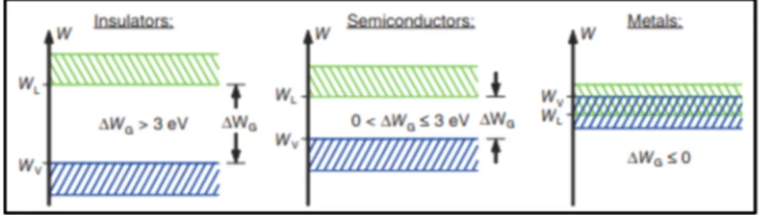
To cross the forbidden zone an amount of energy ΔW_G is absorbed or emitted. It is called bandgap. Depending on the width of the forbidden zone, three types of material are distinguished: insulators, conductors and semiconductors (Figure 1.2).

Figure 1.2: Description of energy band of insulators, conductors and semiconducters - from (Konrad Mertens, 2014)

Insulators are materials with a very big bandgap: typically, more than 3eV. Materials having a bandgap between 0 and 3eV are called semiconductors and materials with negative bandgap are conductors. Metals can be cited as perfect example of conductors.

Table 1.1: Different types of materials - from (Konrad Mertens, 2014) Material Type of material Bandgap ΔW_G(eV)

Diamond Insulator 1.3

Gallium Arsenide Semiconductor 1.42

Silicon Semiconductor 1.12 Germanium Semiconductor 0.7 So, one can see that silicon is not the best conductor. To increase its conduction, a doping

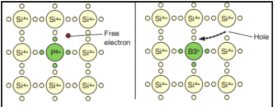
process is applied. This process consists of introducing foreign atoms into a semiconductor. One talks about n-doping when the foreign atom has more valence electrons than the origins atoms. If the foreign atom has less valence electron one talks about p-doping. In the silicon case, Phosphor is often used for n-doping and Boron for p-doping.

Figure 1.3: Phosphor and Boron respectively used for n-doping and p-doping of the Silicon

- from (Konrad Mertens, 2014)

As showed in Figure 1.3, four Phosphor valence electrons link with four Silicon valence electrons. The remaining Phosphor electron is very weakly linked to the nucleus and thus considered as a free electron. It required a very few amounts of energy to transfer this electron to the conduction band. By repeating this process, the semiconductor gains a higher level of conductivity. Regarding the p-doping, the three Boron electron link with three Silicon electrons what leaves one unfilled hole. As a result, one obtains in one side a semiconductor electrically neutral with doped number of free electrons, and in the other side a semiconductor electrically neutral with doped number of holes. The combination of these latter gives a p-n junction.

Once the p-n junction is built, two phenomena take place. Due to the concentration gradient, the free electrons of the n-doped crystal migrate to the p-doped side to fill the hole. It creates a current called diffuse current. The doped crystals are then no longer electrically neutral. The n-doped side is now positively charged while the p-doped side is negatively charged. Due to the rising number of these charges, an electrical field comes into existence. The tendency of this field is to turn back the electrons and the holes to their initial position. This latter electron’s displacement caused field current. Finally, the diffuse and the field current cancelled each other causing the creation of a space charged region at the p-n junction. Figure 1.4 perfectly illustrates this phenomenon.

Figure 1.4: p-n junction - from (Konrad Mertens, 2014)

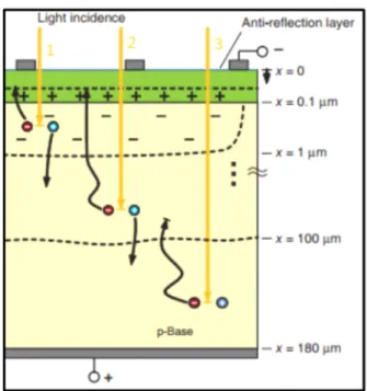
The difference of potential between the n-doped and the p-doped of the space charged region is called diffuse voltage V . When the p-n junction is illuminated, absorbed photons extract _D electron-hole pairs. Depending on the position of the generated pair, three scenarios can be considered. In the space charge region, the electron is separated from hole by the prevailing field. The electron is transferred in the n-doped region and the hole in the p-doped region. Being the majority carriers in these two respective regions, the probability of recombination is very low. Thus, they can easily flow to the contacts. The second scenario is an electron-hole pair located in the space extending 100um after the space charge region. In this case, the charge carrier firstly diffuses to the space charge region. If the pair was in the p-doped side, the electron will diffused. If it was in the n-doped side, the hole will diffused. The diffusion being relatively small, the charge carrier has great chance to reach the space charge region. Once this latter is reached, the first scenario is repeated. If the electron-hole pair extraction takes place beyond 100 um region, the charge carrier will unfortunately recombine before it can reached the space charge region. This migration process is illustrated in Figure 1.5

If a generator reference-arrow system is adopted to describe the previous phenomenon, a p-n junction is called PV solar cell. Otherwise, in load reference-arrow system it is called a photodiode. As showed in Figure 1.6.

Figure 1.5: Electron migration description - from (Konrad Mertens, 2014)

Figure 1.6: Solar cell and Photodiode

1.1.2 PV generator modelling

1.1.2.1 Simple models

The following models are called simple because only manufacturer data are used for very basic mean of calculation. Several ones can be found in the literature; only three of them are presented in this work.

In the first model, the efficiency η is assumed to be a linear function which only depends on the cell temperatureT . If _{c η0} is considered as the nominal efficiency given by the manufacturer and T (25°C) the reference temperature at which this efficiency was measured, the PV 0 generated power P is then given by equation 1.1. _PV

0[1 ( 0)]

PV T c T

P =_ηI =_η −_μ T T I− (1.1)

In the case where the PV nominal power PPV₀ is given, a very closed model shown in equation 1.2 is used. 0 [1 ( 0)] 0 1000 1000 T T PV PV c PV I I P _{= η}P _{= −μ} T T P₋ (1.2)

The third model was proposed by (Lasnier and Gan 1990). It consists of a linear model for the calculation of the maximum powerPmp. The voltage and the current temperature coefficients

OC

V

μ and μ are required to calculate the voltage and the current at the maximum power point. ISC

These latter are given by the equations 1.3,1.4 and 1.5.

mp mp mp

P =V I (1.3)

, OC( , )

mp mp ref V c c ref

, , ( ) SC( , )

T

mp mp ref sc ref I C C ref

ref I I I I T T I μ = + + − (1.5) 1.1.2.2 Electrical model

To predict the power generated by a PV module under certain condition, three electrical equivalent circuits were developed (Mertens, 2014): a simplified model, a standard model also called five parameter model and a two diodes model. The simplified electrical model (Figure 1.7) assumes that a PV solar cell can be modelled as a current generator wires in parallel with a diode.

Figure 1.7: Solar cell simplified electrical model -from (Konrad Mertens, 2014)

The main equation expressing this model is the equation 1.6:

( ) *( f T 1) V m V PH D PH S I =I −I =I −I e − (1.6)

where I , the photocurrent, _PH I the diode saturation current, _s m_f an ideality factor allowing to be closer to reality and V the voltage temperature defined by the equation 1.7. _T

*T T k V q = (1.7)

To go deeper into electrical losses, the standard model also called a five parameters model (Figure 1.8) – was built. In this latter, series resistances R are used to model ohmic losses. _S Leak current at the edge of the solar cell are modelled with the shunt resistanceR . The _SH current is given by the equation 1.8.

PH D SH

I I= − −I I (1.8)

where I is found as: _SH S SH SH V IR I R + = (Mertens, 2014) So, the current I becomes in equation 1.9.

( ) *( 1) S T V IR mV S PH S SH V IR I I I e R + + = − − − (1.9)

Due to its implicit form this equation can only be solved numerically. A complete resolution process is presented by (Duffie and Beckman, 2014).

Figure 1.8: Standard model or five parameters model -from (Konrad Mertens, 2014)

The electron-hole pair recombination process is supposed to be inexistent in the standard model. It was considered in the two diodes model (Figure 1.9). The first diode with an ideality

factor of 1 represents the diffuse current. The second one with the ideality factor of 2 represents the recombination current.

Figure 1.9: Two diodes model -from (Konrad Mertens, 2014)

The characteristic curve equation becomes the equation 1.10.

1 2 2. . *( 1) *( 1) S S T T V IR V IR V V S PH S S SH V I R I I I e I e R + + + = − − − − − (1.10)

The complexity of its solving process made the two diodes model unsuitable to use in PV system yearly simulation. It is mostly used in the research laboratory where more level precision is needed.

1.1.2.3 Sandia PV array Performance model

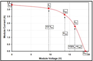
Sandia proposes an empirical array performance model. In their 2004 report (King, Boyson & Kratochvill, 2004), they presented the modelling and the testing of a 165-Wp multi-crystalline silicon module. It took place in Albuquerque during the month of January with both clear and cloudy operating conditions. The model is based on the determination of five different points of the I-V characteristic curve of the studied module as shown in Figure 1.10.

Figure 1.10: Module I-V curve showing the 5 points given by the Sandia performance model

-from (King, Boyson & Kratochvill, 2004),

The first three points correspond to the short circuit currentI , the open circuit voltage _sc V _oc and the maximum pointImp,Vmp. The fourth and fifth equations are defined by their currents

x

I and I and their voltages which respectively correspond to one half of the open circuit xx voltage (1 )

2Voc and the midway between the open circuit voltage and the maximum power point voltage ( (1 ))

2 Voc+Vmp The Fill Factor FF and the maximum power Pmpare then deduced. In these equations, four different aspects are considered: the solar irradiance, the solar resources, the standard conditions and temperature.

A couple of coefficients are defined to account for the solar irradiance influence. They are empirically determined to relate the effective solar irradiance E respectively to_e I_mp,V_mp,I _x andI . _xx

Concerning the solar resources, two empirical functions are used. The function f AM ₁( _a) quantifies the influence of the solar spectral on I . The second function _sc f₂(AOI) quantifies

the optical influence on I . Series of tests are performed to determine their polynomial forms _sc which are (King, Boyson & Kratochvill, 2004) given by the equations 1.11 and 1.12.

2 3 4

1( a) 0 1* a 2*( a) 3*( a) 4*( a)

f AM =a +a AM +a AM +a AM +a AM (1.11)

𝑓 (𝐴𝑂𝐼) = 𝑏 + 𝑏 ∗ 𝐴𝑂𝐼 + 𝑏 ∗ (𝐴𝑂𝐼) + 𝑏 ∗ (𝐴𝑂𝐼) +

𝑏 ∗ (𝐴𝑂𝐼) + 𝑏 ∗ (𝐴𝑂𝐼) (1.12)

The standard conditions are taken for a solar irradiance of 1000 W/m2_{, a temperature of 25°C,}

an air mass of 1.5 and an angle of incidence of 0°.

Regarding the temperature, SANDIA (King, Boyson & Kratochvill, 2004) proposes to first calculate the back-surface module temperature T with the equation 1.13: _m

* *[ea b WS]

m i a

T ₌E + ₊T _(1.13)

where T is the ambient temperature, WS the wind speed measured at 10 m of height, _a E the _i measured irradiance and a and b empirically determined coefficients.

The cell temperature is obtained with the equation 1.14:

* c m o E T T T E = + Δ (1.14)

where ΔT is the temperature difference between the cell and the module back surface temperature at an irradiance of 1000 W/m2_{. The empirically determined coefficients were}

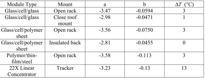
Table 1.2: Empirically determined coefficient were determined for certain module types and mounting configuration -from (King, Boyson & Kratochvill, 2004)

Module Type Mount a b ΔT (°C)

Glass/cell/glass Open rack -3.47 -0.0594 3

Glass/cell/glass Close roof mount -2.98 -0.0471 1 Glass/cell/polymer sheet Open rack -3.56 -0.0750 3 Glass/cell/polymer sheet Insulated back -2.81 -0.0455 0 Polymer/thin-film/steel Open rack -3.58 -0.113 3 22X Linear Concentrator Tracker -3.23 -0.13 13

Once the temperature is calculated, its influence on the cell’s behaviour is implemented by use of temperature coefficients. SANDIA (King, Boyson & Kratochvill, 2004), proposes four temperature coefficients:

sc

I

α ,αImp,β and Voc βVmp. They respectively represent the normalized

temperature coefficient forI , the normalized temperature coefficient for_sc Imp, the temperature coefficient for the module open circuit voltage V as a function of the effective irradiance and _oc the temperature coefficient for module maximum power voltage Vmp as a function of the effective irradiance. SANDIA supposes that taking the same temperature coefficient for I_mp

and I or for _sc V_mp and V ,as in the five parameter model, is erroneous. If not procured by the _oc manufacturer, the four different coefficients must be measured. The whole model equations are presented in APPENDIX A.

1.2 POA (Plane of Array): Radiation modelling 1.2.1 Definitions

Several definitions used in the literature to study the different aspect of solar radiation are needed to understand the gist of the code that was implemented herein. The material presented here was taken from the work of (Duffie and Beckman, 2014).

The solar constant G is the annual average of incident radiation received from the sun _SC outside the earth atmosphere per surface unit. It is estimated at about 1367 W/m2_{. The daily}

extraterrestrial radiation incident on a plane surface is notedG . Its value is given the equation _on 1.15. 360 *(1 0.0033*cos ) 365 on SC n G ₌G ₊ (1.15)

where n is the day of the year

For calculation linked to the position of the sun the standard time is not enough representative. Thus, the solar time is used. It is deduced from the standard time by applying two corrections. The first one is linked to the difference in longitude between the local standard time-based meridian and the observer’s meridian. The second one is from equation time. It gives the equation 1.16.

Solar Time Standard Time 4(= + L_st−L_loc)+ E_t (1.16)

where L is the local meridian for the local time and _st L is the longitude of the location. _loc E _t is the equation of time which is given by the equation 1.17.

229.2*(0.000075 0.001868*cos 0.032077*sin 0.014615*cos 2 0.04089*sin 2 ) t E B B B B = + − − − (1.17)

where B defined the equation 1.18.

360 ( 1)

365

B_{= −}n (1.18)

15*(Solar Time)

ω = (1.19)

The Air mass m is the ratio of the mass of air traverse by the beam radiation at any moment and any location. It is calculated with the equation 1.20.

1 cos z

m

θ

= (1.20)

where θzis the azimuth angle defined later.

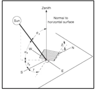
To describe the geometric relationship between the sun position and the earth, several angles must be used (Figure 1.11). The declination angle δ is the angular position of the sun to the solar noon. It is calculated with the equation 1.21.

284 23.45*sin(360 )

365 n

δ = + (1.21)

The latitude _{φ is the angular position in the north and the south of the equator. 90−} o _{≤ ≤φ} 90o . The slope β is the angle formed by the PV array with the horizontal. 0o 180o

β

≤ ≤ . The

azimuth angle _{γ is the horizontal projection of the angle between normal to the surface and} the south. γ_Sis the solar azimuth angle. It is given by the equation 1.22.

1 cos sin sin

( ) cos ( ) sin cos z s z sign θ φ δ γ ω θ φ − − = (1.22)

The angle of incidence _θ is the angle between beam radiation and the normal to the surface. It is given by the equation 1.23.

cos sin sin cos cos cos sin sin sin

θ δ φ β δ φ β γ δ φ β ω

δ φ β γ ω δ β γ ω

= − +

+ + (1.23)

The zenith angle θ_z is the angle between the line to the sun and the vertical. Its complementary S

α is the angle between the line to the sun and the horizontal. The angle of incidence is equal to the zenith angle for horizontal surface. This comes to put β equal to zero in the previous equation. It gives the equation 1.24.

cos_θz =cos cos cos_{φ δ ω}+sin sin_{φ δ} (1.24)

Figure 1.11: Solar angle -from (Duffie & Beckman, 2014)

1.2.2 Estimation of solar Radiation

The extraterrestrial radiation calculated upper is not totally transferred to the earth. In fact, one part of this energy is absorbed by the atmosphere, deviated or scattered. This is called the diffuse radiation. The other part which directly reached the earth surface is the beam radiation.

Different empirical models were developed to estimate these two entities in an hourly, daily or monthly basis.

1.2.2.1 Beam and Diffuse radiation estimation

(Hottel, 1976) presents a model to calculate the beam radiation through the atmosphere. It is based on the calculation of the atmosphere transmittance for beam radiation τ_b which is the ratio of beam radiation to the extraterrestrial radiation on a horizontal surface. It is given by the equation 1.25. cos 1* z k b ao a e θ τ = + − (1.25)

The constantsa , ₀ a and k are calculated for a standard atmosphere with 23 km of visibility. ₁ They are deduced from the reference constants *

0

a , * 1

a and _k* _{that are drawn from the} equations 1.26, 1.27 and 1.28. * 2 0 0.4237 0.00821*(6 ) a = − −A (1.26) * 2 1 0.5055 0.00595*(6.5 ) a = − −A (1.27) * _{0.2711 0.01858*(2.5 )}2 k = − −A (1.28)

where A is the altitude in km

In the Table 1.3 are given the correction factors 0 0 * 0 a r a = , 1 1 * 1 a r a = and r_k k_* k = .

Table 1.3: Correction factor -from (Duffie & Beckman, 2014)

Climate Type r ₀ r ₁ r _k

Tropical 0.95 0.98 1.02

Subarctic summer 0.99 0.99 1.01

Midlatitude winter 1.03 1.01 1.00

Keeping the same line, (Kreith and Kreider, 1978) proposed a different atmosphere transmittance for beam radiationτ_b. In this case, the curvature of the light rays is considered. It is obtained with the equations 1.29, 1.30 and 1.31.

0.65m(z, ) 0.095 ( , ) 0.5*( z m z z ) b e θ e θ τ ₌ − ₊ − _(1.29) (z) ( , ) (0, ) , : (0) z z p m z m p atmospheric pressure p θ = θ (1.30) 2 (0, )_z 1229 (614cos )_z 614cos _z m _{θ = + θ − θ} (1.31)

After estimating the beam radiation, it is important to calculate the diffuse radiation on a horizontal surface and then deduce the total radiation. (Liu and Jordan, 1960) bring out an empirical relation between the atmosphere transmittance for beam and diffuse radiation τ_band

d

τ . Equation 1.32 traduce this model.

0 0.271 0.294* d d b I I τ = = − τ (1.32)

Thus, by combining Liu and Jordan model and Hottel model, one can deduced the total irradiation on a plane surface.

1.2.2.2 Correlation of Erbs

With the advance measurement’s techniques, other researchers tried to establish more precise models. It is the case of (Erbs and al, 1980). To estimate the ratio of hourly diffuse radiation, they proposed to correlate the hourly clearness k and the diffuse fractionT d

I

respectively: the diffuse radiation on a plane surface and the hourly total radiation. k is defined _T by equation 1.33. 0 T I k I = (1.33)

where I the extraterrestrial radiation on a horizontal surface for an hour period. It is calculated ₀ with the equation 1.34.

0 2 1

2 1

12*3600 360

(1 0.033cos )[cos cos (sin sin ) 365 ( ) sin sin ] 180 sc n I G φ δ ω ω π π ω ω _{φ δ} = + − − + (1.34)

The Erbs and al correlations are shown in the equation 1.35.

2 3 4 1 0.09 0.22 0.9511 0.1604 4.388 16.638 12.336 0.22 0.8 0.165 0.8 T T d T T T T T k for k I k k k for k I for k − ≤     = − + − + < ≤   _>    (1.35)

The same correlation is also available in a daily or monthly basis with K the daily clearness _T and K the monthly clearness. They are respectively defined as the ratio of the total radiation _T

H to the extraterrestrial radiation on a horizontal surface H in a daily basis and the ratio of 0 the monthly global radiation H to the extraterrestrial radiation on a horizontal surface H in ₀ a monthly basis. H and ₀ H0 given by the equation 1.37.

0

24*3600* 360

(1 0.033cos )[cos cos sin sin sin ]

365 180 SC s s G n H _{φ δ ω} πω _{φ δ} π = + + (1.36)

0, 1 0 i i H H N = =



where N is the number of days in the month and H_0,ithe extraterrestrial irradiation at the ith day of the month. Knowing the value ofK , if the sunset hour angle _{T ωs} is inferior or equal to 81.4, the correlation is given the equation 1.38.

2 3 4 1 0.2727 2.4495 11.9514 9.3879 0.715 0.143 0.715 T T T T T d T K K K K for K H H for K  _{− + − + <}  =   ≥  (1.38)

Otherwise the equation 1.38.

2 3 1 0.2832 2.5557 0.8448 0.715 0.175 0.715 T T T T d T K K K for K H H for K  _{+ − + <}  =   ≥   (1.39)

In a monthly basis, the calculation of K leads to the equation 1.40. _T

2 3 2 3 1.391 3.560 4.189 2.137 81.3 0.3 0.8 1.311 3.022 3.427 1.821 81.3 0.3 0.8 T T T s T d T T T s T K K K for and K H H _{K K K for and K} ω ω  _{− + − ≤ ≤ ≤}    =    − + − > ≤ ≤    (1.40)

Thus, Erbs and al. correlation allows calculating the diffuse radiation by knowing the clearness. The beam radiation is then deduced by subtracting the diffuse part from the global radiation. Most of the time, hourly correlation is used as this latter insured to have more precise results. But, most of the time, due to the lack of data, only daily or even monthly global radiations are available. To solve this issue, (Collares-Pereira & Rabl, 1979) propose a method to deduce the hourly total radiation I from the daily total radiation H. The ration of hourly total radiation to daily total radiation r is firstly calculated by the equations 1.41, 1.42 and 1.43. _t

cos cos ( cos ) 24 _{sin cos} 180 s t s s s r π a b _ω ω ω πω ω ω − = + − (1.41) 0.409 0.5016*sin( _s 60) a= + _ω − (1.42) 0.6609 0.4767*sin( s 60) b= − ω − (1.43)

Then knowingH, I is deduced.

1.2.2.3 Radiation on sloped surface

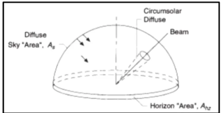
Till now, all the calculations were done for horizontal surface. But, especially for PV installations, the surface in question is sloped. So, it is very important to know the solar radiation incident on a tilted surface. In this case, not only the diffuse and beam radiation are considered. The radiation reflected from different surfaces “seen” by the tilted surface is included. As showed in Figure 1.12, the diffuse radiation is separated in three parts: the isotropic part I_{T d iso,} received uniformly, the circumsolar diffuse part I_{T d cs,} and the part coming from horizon brightening I_{T d hz,} .

Figure 1.12: Diffuse radiation model for tilted surface -from (Duffie & Beckman, 2014)

,b , , , ,

T T T d iso T d cs T d hz T r

I =I +I +I +I +I (1.44)

whereI_T,bandI_T,r respectively: the beam radiation on tilted surface and the reflected radiation on the tilted surface.

This equation can also be written like equation 1.45.

, , ,

T b b d iso c s d cs b d hz c hz g c g

I =I R +I F− +I R +I F− +Iρ F− (1.45)

whereF_{c s−} , F_{c hz−} and Fc g− respectively the view factor from the sky to the collector, the view factor from the horizon to the collector and the view factor from the ground to the collector.

g

ρ is the albedo. The geometric factorR , the ratio of beam radiation on tilted surface to that b of a horizontal surface at any time, can be calculated with the equation 1.46.

, , cos cos T b b hor b z I R I θ θ = ≈ (1.46)

The different models found in the literature aimed to explicitly define the view factors. The simplest model is the isotropic sky model (Shukla, Rangnekar & Sudhakar, 2015). In this latter, only the isotropic share of the diffusion radiation is considered. It is given by the equation 1.47.

1 cos 1 cos

*( ) * ( )

2 2

T b b d g

I ₌I R ₊I + β ₊I _ρ − β (1.47)

where β is the tilted angle.

An anisotropic model proposed by (Hay and Davies, 1980) separates the diffuse in two parts: the isotropic and the circumsolar. The diffuse radiation is written is obtained from with equation 1.48:

, , , 1 cos [(1 )( ) ] 2 d T T d iso T d cs d i i b I ₌I ₊I ₌I ₋A + β ₊A R (1.48)

where A is the anisotropic index which is given by the equation 1.49. _i

0 b i I A I = (1.49)

The total radiation on a tilted surface is then given by the equation 1.50.

1 cos 1 cos

( ) (1 )( ) ( )

2 2

T b d i b d i g

I ₌ I ₊I A R ₊I ₋A + β ₊I_ρ − β (1.50)

To take into account the horizon brightening, (Reindl and al., 1988) add a modulating factor 3

1 sin ( ) 2

f β

+ where f is defined by the equation 1.51.

b

I f

I

= (1.51)

The diffuse on a tilted surface is given by the equation 1.52.

3 , 1 cos [(1 )( )(1 sin ( )) ] 2 2 d T d i i b I ₌I ₋A + β ₊ f β ₊A R (1.52)

So, the complete model named as HDKR (Hay, Davies, Klutcher and Reindl) gives the equation 1.53.

3 1 cos 1 cos ( ) (1 )( )(1 sin ( )) ( ) 2 2 2 T b d i b d i g I ₌ I ₊I A R ₊I ₋A + β ₊ f β ₊I_ρ − β (1.53) Battery 1.3 Battery technology

A deep description of the different phenomena and reactions occurring into batteries was made by (Mark, 2014). A summary of this work is provided is in this paragraph. Batteries are made with electrochemical cells. They convert chemical energy into electricity. Battery cells are made with two electrodes deepen in an electrolyte solution. The current flows when the circuit is closed. Chemical reactions occurring between the electrodes and the electrolyte made current flows. The electrodes and the electrolyte might differ depending on the types of batteries. In the market can be found: lead acid batteries, lithium ion, nickel metal hybrid and nickel cadmium. Lead acid battery being more readily available and cost effective, its use is more suitable for remote area. For this latter, the redox reaction operates between lead dioxide plate (PbO ), a negative lead plate ( Pb ) and an electrolyte composed with of sulphuric acid (₂

2 4 H SO ). 2 2 4 4 2 Charge 2 2 2 Discharge Pb PbO H SO PbSO H O ← + + ⇔ + → (1.54)

During the charging, lead dioxide is produced on the positive plate, lead is produced on the negative plate and the amount of sulphuric acid increased. When the battery is being discharged, lead sulphate is produced, and the water increased. When fully charged, the cell battery voltage is 2.1 V.

A battery can store a certain amount of energy which is its capacity. Transmitted by the manufacturer, it is measured in Ah. Its value varies with the rate at which the battery is discharge. A discharge current of 1amp might deliver 100 Ah which give a capacity of 100Ah.

The same battery which discharges with a current of 4 amps has a rated capacity of 80Ah. But the whole capacity of the battery can’t be used. A depth cycle battery should not be discharged below 60%. The admissible minimum level of energy is called maximum depth of discharge (𝐷𝑜𝐷 ). To insured that this threshold is not reached, the state of charge (𝑆𝑂𝐶) of the battery must be controlled. Beyond its discharge, the battery loses charge by a process called self-discharge.

An overcharge occurs when a battery at 100% of state of charge is still in charge. Continued overcharge can reduce the lifetime of the battery. In fact, the excess current causes a reaction into the battery that converts the water in hydrogen. This decreases the amount of electrolyte and liberates explosive hydrogen gas in the air. To avoid this phenomenon, a charge controller is always connected between the battery and PV array or the DC bus depending on the configuration of the system.

1.3.1 Battery modelling

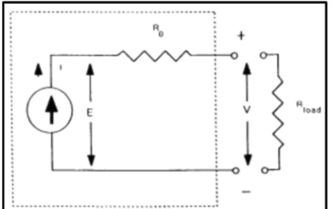
In general, a battery is viewed as a voltage source in series with a resistance, as illustrated in Figure 1.13. Depending on the required level of precision, different approach can be found. Analytical model have the advantage to be general, but some taken hypothesis makes the obtained solutions non-representative of the whole reality. In parallel, empirical models based on experimental results exist. Most of them required parameters that are not given by the manufacturer. Three different models are exposed in this review: the KiBaM model (Manwell & McGowan, 1993), the CIEMAT model (Coppeti, Lorenzo & Chenlo, 1993) and the Pspice model (Ameen, Pasupuleti & Khatib, 2015).

Figure 1.13: Battery electrical schematic -from (Coppeti, Lorenzo & Chenlo, 1993)

1.3.1.1 Kinetic Battery Model (KiBaM)

The KiBaM model (Manwell & McGowan, 1993) is based on the chemical kinetics’ behaviour of the battery. The voltage source is modelled as two tanks separated with a conductance. The immediately available charge is modeled as a tank having a capacity, q . The bound charge is 1 represented by a second tank with a capacity q . The equations 1.55 and 1.56 traduce this ₂ modelling. 1 1 2 '( ) bat dq I k h h dt = − − − (1.55) 2 1 2 '( ) dq k h h dt = − (1.56)

where I is the constant current during a time step, '_bat k the conductance, h and ₁ h the ₂ heads of the two tanks ( Figure 1.14).

Figure 1.14: Kinetic Battery model - from (Manwell & McGowan, 1993)

If q1,0and q2,0are taken as the initial amount of charge, the resolution of these equations leads to the equations 1.57 and 1.58.

0 2 1,0 ( )(1 kt) ( 1 kt) kt q kc I e Ic kt e q q e k k − − − − − − + = + − (1.57) 2 2,0 0 (1 )( 1 ) (1 )(1 ) kt kt kt I c kt e q q e q c e k − − − − − + = + − − − (1.58)

where c is the width of the first tank and 1 c_{− the width of second tank (Figure 1.14).} The constantq1,0, c and k are than to be defined. The proposed resolution process is developed in the APPENDIX B. One can noticed that the temperature effect is not taken into account by this model.

1.3.1.2 CIEMAT model

In the CIEMAT’s laboratory, a general battery model for PV system simulation was developpe by (Coppeti, Lorenzo & Chenlo, 1993). Its normalization with respect to the battery capacity allows the generalization of the model to different size of battery. Three types of operating mode are modelled: the discharging mode, the charging mode and the overvoltage mode.

Contrary to KiBaM model, the temperature effect is taken into account. This makes it suitable for regions which go through high temperature during the year.

Thus, the discharge voltage variation with the state of charge SOC is given by the equation 1.59. 1.3 1.5 10 4 0.27 [2.085 0.12(1 )] ( 0.02)(1 0.007 ) 1 bat d bat I V SOC T C I SOC = − − − + + − Δ + (1.59)

where I is the discharge current and _{bat Δ}Tthe temperature variation regarding the reference temperature 25°C. The depth of discharge DOD is the ratio of the charge Qgiven by the battery to the battery capacity C at a given time. The state of charge SOC as a complement of DOD is given by the equation 1.60.

1 1 Q

SOC DOD

C

= − = − (1.60)

The capacity is calculated by the equation 1.61.

0.9 10 10 1.67 (1 0.005 ) 1 0.67( ) C T I C I = + Δ + (1.61)

The equation is normalized with regard to discharge current Ibat,10 corresponding to the rated capacityC . 10

Similarly, the charging voltage is calculated by the equation 1.62.

0.86 1.2 10 6 0.48 [2 0.16* ] [ 0.036][1 0.025 T] 1 (1 ) bat c bat I V SOC C I SOC = + + + + − Δ + − (1.62)