HAL Id: hal-01348978
https://hal.archives-ouvertes.fr/hal-01348978
Submitted on 29 Jul 2016
HAL is a multi-disciplinary open access
archive for the deposit and dissemination of
sci-entific research documents, whether they are
pub-lished or not. The documents may come from
teaching and research institutions in France or
abroad, or from public or private research centers.
L’archive ouverte pluridisciplinaire HAL, est
destinée au dépôt et à la diffusion de documents
scientifiques de niveau recherche, publiés ou non,
émanant des établissements d’enseignement et de
recherche français ou étrangers, des laboratoires
publics ou privés.
Anisotropic Scale Space
Maxim Karpushin, Giuseppe Valenzise, Frédéric Dufaux
To cite this version:
Maxim Karpushin, Giuseppe Valenzise, Frédéric Dufaux. Keypoint Detection in RGBD Images Based
on an Anisotropic Scale Space. IEEE Transactions on Multimedia, Institute of Electrical and
Elec-tronics Engineers, 2016, �10.1109/TMM.2016.2590305�. �hal-01348978�
Keypoint detection in RGBD images based on an
anisotropic scale space
Maxim Karpushin, Student Member, IEEE, Giuseppe Valenzise, Member, IEEE, Fr´ed´eric Dufaux, Fellow, IEEE,
Abstract—The increasing availability of texture+depth (RGBD) content has recently motivated research towards the design of image features able to employ the additional geometrical infor-mation provided by depth. Indeed, such features are supposed to provide higher robustness than conventional 2D features in presence of large changes of camera viewpoint. In this paper we consider the first stage of RGBD image matching, i.e., keypoint detection. In order to obtain viewpoint-covariant keypoints, we design a filtering process, which approximates a diffusion process along the surfaces of the scene, by means of the information provided by depth. Next, we employ this multiscale representation to find keypoints through a multiscale keypoint detector. The keypoints obtained by the proposed detector provide substantially higher stability to viewpoint changes than alternative 2D and RGBD feature extraction approaches, both in terms of repeatabil-ity and image classification accuracy. Furthermore, the proposed detector can be efficiently implemented on a GPU.
Index Terms—RGBD, texture+depth, local features, keypoints, SIFT, anisotropic diffusion.
I. INTRODUCTION
Local image features represent a key tool in a number of practical scenarios and applications in multimedia, including visual search [2], classification [3], indexing [4], image anal-ysis [5], etc. Several comparative evaluations of local features have appeared in the past decade [6], [7], [8], [9], [10], [11], [12], [13], in response to the increasing research interest in this field. At the same time, the industrial demand for robust, distinctive and compact visual features has stimulated MPEG standardization activities for Compact Descriptors for Visual Search (CDVS) [14] and Compact Descriptors for Visual Analysis (CDVA) [15].
While 2D visual features have nowadays achieved a substan-tial level of maturity in terms of robustness, compactness, and efficiency, the emergence of richer image and video formats, such as texture+depth (RGBD), multiview or plenoptic images, have recently attracted attention towards the definition of features able to capture and leverage the geometric information of a scene [1], [16], [17]. Indeed, acquiring scene geometry is nowadays feasible with low-cost devices, such as Microsoft Kinect [18], Asus Xtion [19], Structure Sensor, or even mobile devices such as HTC One M8 and the upcoming Google Tango, which are capable of acquiring depth together with conventional color images.
The availability of geometrical information provided by depth could help to improve the performance of current image
The authors are with the Laboratoire Traitement et Communication de l’Information (CNRS LTCI), T´el´ecom ParisTech, Universit´e Paris Saclay (e-mail: {firstname.lastname}@telecom-paristech.fr). Part of this work has been presented at the IEEE International Conference on Multimedia and Expo, 2015 [1].
matching techniques in the presence of large variations of the camera viewpoint, where conventional feature schemes fail to detect and match repeatable keypoints [1], [20], [21]. In our previous work [16], [20] we have shown that depth information can be successfully used in the computation of local descriptors, by locally resampling texture images based on depth maps in such a way to “un-slant” [16] or unwrap [20] object surfaces in the camera plane. In this way, we achieve a sort of viewpoint normalization on image patches prior to their descriptor computation. However, this process is done around keypoints found using texture only, i.e., depth is ignored during keypoint detection.
In this paper we consider instead the first stage of the image matching problem, i.e., the extraction of repeatable RGBD keypoints, making use of the available depth information. Specifically, this paper presents two contributions. First, we present an image smoothing filter that exploits the information provided by depth in order to produce a scale space for the texture map. Second, we propose a keypoint detector for texture+depth images that uses the designed scale space as the keypoint detection modality. The proposed detector aims at improved keypoint repeatability under viewpoint position changes.
In our preliminary work [1], we proposed a diffusion process for RGBD data and proved that it engenders a scale space, suitable for keypoint detection. This paper extends the construction in [1] by addressing its two main limitations:
∙ The proposed scale space was initially tested with the standard SIFT detector which is, however, not optimal for the proposed scale space. In the present paper, we propose a new detection scheme adapted to the proposed scale space allowing for better performance on real data.
∙ The initially proposed diffusion process is
computation-ally expensive. In the present paper, we propose and test a GPU implementation allowing for a substantial speed up (tens of times with respect to our previous work). Moreover, in this paper we test the entire proposed keypoint detection scheme not only on synthetic RGBD data, but also on real RGBD images that we captured using a Kinect sensor. The rest of the paper is organized as follows. In Section II, we present related work on local features for 2D images and texture+depth content, as well as background concepts on scale space construction in the context of keypoint detec-tion. Section III discusses the proposed scale space definition using a diffusion process, while Section IV describes how to design a keypoint detector based on the proposed scale space. In Section V, we present experimental results, including repeatability score on synthetic RGBD images and a scene
recognition application scenario on a set of Kinect images. Finally, Section VI concludes the paper.
II. BACKGROUND AND RELATED WORK
A. Image matching through local features
Sparse image matching is a basic task for a number of problems in vision. It consists of three main steps: (i) detection of interest points (keypoints), (ii) local description of all detected keypoints, and (iii) descriptors matching. In this paper, we focus on the first step of the image matching, whose goal is to produce keypoints that are repeatable, i.e., reproduce their locations in the image as independently as possible from noise and different kinds of visual deformations, especially viewpoint position changes.
A number of scale and rotation-invariant local features have been proposed in the literature during the past decades. Scale-Invariant Feature Transform (SIFT) [22], Speeded Up Robust Features (SURF) [23] and binary features [24], [25] represent some of the most successful examples of robust application-independent local image features allowing for efficient sparse image matching.
Most of these features are invariant or exhibit high robust-ness to scale changes and in-plane rotations, which is generally sufficient in many image matching scenarios. However, in some applications such as indoor localization or visual odom-etry, images could undergo more complex deformations, such as viewpoint position changes, perspective distortions or out-of-plane rotations. At the image feature extraction level, these deformations combined with in-plane translations, rotations and scale changes are commonly considered as equivalent (for these reason, we further refer to it as viewpoint position changes). For conventional feature extractors that use only 2D information, this type of deformations is challenging. For example, the authors of [22], [26] have found that out-of-plane rotations larger than 40° entail a substantial decrease in SIFT matching performance.
A common way to deal with out-of-plane rotations consists in approximating the perspective distortions by local affine transformations. Harris and Hessian affine-covariant detec-tors [27], [28] based on an iterative procedure allow to estimate a keypoint neighborhood by a local affine shape. Before the de-scriptor extraction, the corresponding local patch undergoes an affine normalization, consisting in applying the inverse of the estimated affine transformation. Affine SIFT [26] consists in a simulation of affine transformations instead of a normalization: it samples affinely transformed patches in all keypoints, and then retrieves the most frequent transformations between the two images being matched. A similar affine generalization of SURF is presented in [29].
Affine-invariant features demonstrate better stability with respect to viewpoint position changes. A major limitation of the affine invariance paradigm consists in the fact that it is not able to distinguish between a square and a rectangle, or a circle and an ellipse, as these shapes are equivalent to each other up to an affine transformation [30]. Thus affine invariant features can produce a more robust but less discriminative description compared to standard scale and rotation-invariant features like SIFT [16].
Therefore, dealing with out-of-plane rotations, viewpoint position changes and 3D rigid scene deformations still remain challenging for the repeatability and discriminability of local image features. We believe that the main interest in using an extended modality, i.e., the texture complemented by the depth map, is to address these transformation classes and provide more repeatable and distinctive features.
B. Keypoint detection in RGBD images
A texture+depth (RGBD) image could be considered as a mesh with an associated texture. Thus, RGBD matching could be cast as a problem of mesh matching, for which several techniques have been proposed in the literature, such as the Mesh Difference of Gaussians and Histograms of Oriented Gradients (MeshDoG+MeshHOG) [31], Mesh Local Binary Patterns [32], photometric heat kernel signatures [33]. How-ever, several problems arise in such a setting. First of all, mesh matching techniques are not apt to deal with occlusions that are commonly present in images. Second, a mesh is typically defined in its own coordinates, whereas an RGBD image is given in the camera coordinates. Consequently, any camera displacement corresponds to resampling the observed mesh, which is affected by the acquisition noise and thus hinders the repeatability of detected keypoints. Therefore, image-level techniques for feature detection on RGBD content are of interest.
Viewpoint invariant patches (VIP) [30] exploit the depth map in order to discover dominant planes in the scene and then render their frontal (normalized) views. SIFT features are then extracted from the rendered views. This technique allows for efficient matching of scenes with relatively simple geometry. However, when smooth surfaces or high frequency details are present in the input data, VIP may not perform well. Moreover, VIP uses a RANSAC-based technique to detect the dominant planes, which adds a randomness component in the extracted features, especially in presence of noise in the depth: in some cases, with a non-zero probability VIP may fail to match a given image against itself.
A number of approaches for RGBD content matching do not exploit the depth map at the keypoint detection stage, but use it only to compute descriptors, e.g., Perspective Invariant Normal features (PIN) [34], Binary Robust Appearance and Normal Descriptor (BRAND) [21], Color Signature of Histograms of OrienTations (CSHOT) [35], and our previous work [20]. In these cases, keypoints are typically detected in the texture image only using a conventional keypoint detector, and then described with the aid of depth information. To the authors’ knowledge, there is a lack of RGBD keypoint detectors in the literature. A reason for this could probably be that designing a texture+depth descriptor is a simpler and less constrained problem compared to the design of a texture+depth detector.
Other approaches focus on keypoint detection in depth maps only, such as 2.5D SIFT [36], Normally Aligned Ra-dial Feature (NARF) [37], or Scale Invariant Point Feature (SIPF) [38]. Rejecting the texture information makes keypoint detection invariant to illumination changes and can be useful in privacy-enabled vision applications. Nevertheless, depth maps
alone, without texture, may be not informative enough to provide a rich feature representation for many practical vision applications.
C. Scale spaces
The Gaussian kernel is one of the most common linear image smoothing operators:
𝐾𝜎(𝑥, 𝑦) = 1 2𝜋𝜎2exp (︂ −𝑥 2+ 𝑦2 2𝜎2 )︂ . (1) The kernel separability allows for a faster filter response computation: the 2D convolution may be replaced by a set of 1D convolutions over image lines and columns.
Compared to other common low-pass filters, Gaussian filter is particularly important in computer vision due to certain properties established within the diffusion equation frame-work [39]. Specifically, it is well-known that the partial differential equation (PDE) problem:
⎧ ⎨ ⎩ 𝜕𝑓 𝜕𝑡 = 𝜕2𝑓 𝜕2𝑥+ 𝜕2𝑓 𝜕2𝑦 ≡ Δ𝑓 𝑓 |𝑡=0= 𝑓0 (2)
where Δ𝑓 is the Laplacian operator, possesses a unique solution 𝑓 (𝑡, 𝑥, 𝑦) = (︀𝐾√
2𝑡* 𝑓0)︀ (𝑥, 𝑦), with * denoting
the convolution product. With this setup, where the initial data 𝑓0 represents the input image, a set of properties may
be established for the Gaussian smoothing, proving that a sequence of progressively smoothed images forms a scale space. According to the definition proposed by Koenderink in [40], to be a scale space such a set of images with different scales must satisfy two properties (scale space axioms):
∙ causality (non creation of local extrema), i.e. any feature
at a coarse level of resolution1 is required to possess
a (not necessarily unique) “cause” at a finer level of resolution;
∙ homogeneity and isotropy, i.e. the smoothing is spatially invariant.
The first axiom is crucial for keypoint detection. Thus, the Gaussian scale space is widely used in feature extraction algorithms, including SIFT [22].
A scale space may be defined without involving the second axiom, for example, it can be based on a semantically con-sistent smoothing that preserves the internal image structure (notably, the edges) and still satisfy the causality axiom. The first model of non-linear scale space was proposed by Perona and Malik [41], who formulated a non-linear PDE problem in such a way that the diffusion process is controlled by the image gradient norm. Such a non-uniform scale space concept is further generalized by the anisotropic diffusion filtering, where the diffusivity becomes non-scalar [39], [42], and to the multiscale image representations on manifolds [43]. Such non-uniform scale spaces were successfully applied in feature detection [44], [45], [46].
Differently from the cited works, the proposed approach consists in exploiting the depth map in order to define a non-uniform scale space for the texture image. The process we
1Here resolution means scale and not the image size.
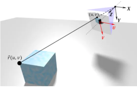
Fig. 1. Scene surface parametrization in local camera coordinates.
define aims at exploiting the surface properties that do not depend on the observer position in order to render a viewpoint-covariant multiscale representation that is able to reveal robust keypoints. To the authors’ best knowledge, this setting has not yet been exploited in feature detection. Moreover, in spite of its non-uniform nature, our scale space remains linear in function of the input texture image (differently from Perona and Malik’s construction [41], for example). Last but not least, we prove that our proposed smoothing filter is numerically stable, which is not always the case for complex scale spaces. For example, Perona and Malik’s smoothing may demonstrate unstable behavior [39].
III. DESIGN OFRGBDSCALE SPACE
A. Laplacian operator definition
We first define a Laplacian operator for RGBD content that enables to establish a diffusion process in such a way to engender a scale space.
Let the input image be of size 𝑊 × 𝐻 pixels, so that Ω = [︀−𝑊 2, 𝑊 2 − 1]︀ × [︀− 𝐻 2, 𝐻
2 − 1]︀ denotes the image support. In
what follows, spatial image variables taking values from Ω are referred to as 𝑢 and 𝑣. We denote by 𝐷 : Ω → R+ the depth
map associated to the image 𝐼 being processed. We assume known the horizontal angle of view 𝜔 of the camera.
It can be easily shown using the pinhole camera model, that the function ⃗𝑟 : Ω → R3defined below parametrizes the image
surface in local camera coordinates as illustrated in Fig. 1:
⃗ 𝑟(𝑢, 𝑣) = ⎛ ⎝ 2𝑢 tan𝜔2 2𝑣𝑊𝐻 tan𝜔2 1 ⎞ ⎠𝐷(𝑢, 𝑣). (3)
Let us now proceed to a discrete image support Ω𝑑obtained
by sampling Ω with step ℎ in both dimensions. For a function 𝑓 defined on the continuous support Ω, we introduce the following differential quantities, which are similar to the notion of directional derivatives in [31]:
𝜕𝑢𝑓 = 𝑓 (𝑢 + ℎ, 𝑣) − 𝑓 (𝑢 − ℎ, 𝑣) ‖⃗𝑟(𝑢 + ℎ, 𝑣) − ⃗𝑟(𝑢 − ℎ, 𝑣)‖ = =𝑓 (𝑢 + ℎ, 𝑣) − 𝑓 (𝑢 − ℎ, 𝑣) 𝑟𝑢+− (4)
𝜕𝑣𝑓 = 𝑓 (𝑢, 𝑣 + ℎ) − 𝑓 (𝑢, 𝑣 − ℎ) ‖⃗𝑟(𝑢, 𝑣 + ℎ) − ⃗𝑟(𝑢, 𝑣 − ℎ)‖ = = 𝑓 (𝑢, 𝑣 + ℎ) − 𝑓 (𝑢, 𝑣 − ℎ) 𝑟+−𝑣 (5) where 𝑟+−
𝑢 and 𝑟+−𝑣 are introduced in order to simplify
notation. Applying twice this operator yields second-order differential quantities, e.g., 𝜕𝑢𝑢𝑓 = 𝜕𝑢(𝜕𝑢𝑓 ). For a better
operator kernel locality, we also introduce a definition through one-sided finite differences as follows:
𝜕𝑢+𝑓 = 𝑓 (𝑢 + ℎ, 𝑣) − 𝑓 (𝑢, 𝑣) ‖⃗𝑟(𝑢 + ℎ, 𝑣) − ⃗𝑟(𝑢, 𝑣)‖ = 𝑓 (𝑢 + ℎ, 𝑣) − 𝑓 (𝑢, 𝑣) 𝑟𝑢+ , (6) 𝜕𝑢−𝑓 = 𝑓 (𝑢, 𝑣) − 𝑓 (𝑢 − ℎ, 𝑣) ‖⃗𝑟(𝑢 − ℎ, 𝑣) − ⃗𝑟(𝑢, 𝑣)‖ = 𝑓 (𝑢, 𝑣) − 𝑓 (𝑢 − ℎ, 𝑣) 𝑟𝑢− , (7) 𝜕𝑢𝑢𝑓 = 𝜕𝑢+𝑓 − 𝜕𝑢−𝑓 𝑟+−𝑢 = 𝑓 (𝑢 + ℎ, 𝑣) 𝑟𝑢+𝑟𝑢+− −𝑓 (𝑢, 𝑣) 𝑟+𝑢𝑟+−𝑢 −𝑓 (𝑢, 𝑣) 𝑟𝑢−𝑟+−𝑢 +𝑓 (𝑢 − ℎ, 𝑣) 𝑟𝑢−𝑟𝑢+− . (8) 𝜕𝑣+𝑓 , 𝜕𝑣−𝑓 and 𝜕𝑣𝑣𝑓 are defined in an analogous way.
Finally, we define a Laplacian-like second order differential operator summing up the second-order differential quantities defined above:
𝐿 ≡ 𝜕𝑢𝑢+ 𝜕𝑣𝑣. (9)
B. PDE problem formulation
Next, we set up a partial differential equation problem that describes the diffusion process with the proposed Laplacian operator (9): ⎧ ⎨ ⎩ 𝜕𝑓 𝜕𝑡 = 𝐿𝑓 𝑓 |𝑡=0= 𝑓0. (10)
This problem is very similar to the classic diffusion problem (2). To study this similarity and set up some useful properties, let us return back to the continuous definition domain. We obtain a continuous generalization of the differential quanti-ties (4) and (8) by letting ℎ tend towards zero, that is:
𝒟𝑢𝑓 = 𝑓𝑢‖⃗𝑟𝑢‖−1
𝒟𝑢𝑢𝑓 = 𝑓𝑢𝑢‖⃗𝑟𝑢‖−2− 𝑓𝑢‖⃗𝑟𝑢‖−4(⃗𝑟𝑢, ⃗𝑟𝑢𝑢) . (11)
Thus, we get the continuous version of problem (10): ⎧ ⎨ ⎩ 𝜕𝑓 𝜕𝑡 = 𝒟𝑢𝑢𝑓 + 𝒟𝑣𝑣𝑓 𝑓 |𝑡=0= 𝑓0. (12)
It is worth noticing that if the depth 𝐷 is constant (i.e., we have a non-informative depth map), this PDE problem becomes equivalent to the classic linear diffusion filtering (2), as the differential operator on the right side of the equation turns into the classic Laplacian up to a constant multiplier due to ⃗
𝑟𝑢 = ⃗𝑟𝑣 ≡ 𝑐𝑜𝑛𝑠𝑡 and ⃗𝑟𝑢𝑢 = ⃗𝑟𝑣𝑣 ≡ 0. This allows for a
“backward compatibility” of the proposed scale space to the classic Gaussian scale space in the case when the depth map
is not provided. Moreover, this property is satisfied locally, i.e., at points where 𝐷 is continuous and the surface normal is parallel to the camera optical axis.
C. Well-posedness, numerical solution and its causality In order to make use of the PDE problem (10), we have to ensure that it has a unique solution that depends continuously on the initial data 𝑓0. This is a fundamental property known
as well-posedness.
To establish the well-posedness of problem (10) we use some of the results of [39]. We rewrite (10) in a vector form, i.e., 𝑓 (𝑡) ∈ R𝑊 ×𝐻 and the application of 𝐿 to 𝑓 is
represented by a matrix multiplication 𝒜𝑓 . The coefficients of matrix 𝒜 depend only on ⃗𝑟 and are explicitly deduced from its definition (8).
First, we apply theorem 4 of [39]. It is straightforward to show that the operator matrix satisfies all the conditions except the symmetry, i.e., it has vanishing row sums (S3), nonnegative off-diagonals (S4) and is irreducible (S5). Lipschitz-continuity (S1) is satisfied unconditionally as 𝒜 does not depend on 𝑓 . The violated condition of the matrix symmetry (S2) is not required for well-posedness and extremum principle, as it is noticed afterwards [39, p. 76].
This proves that not only is the problem well-posed, but that the solution 𝑓 respects the extremum principle allowing to set up the causality. It implies that the resulting filter is causal in spatial image variables, guaranteeing that no spurious features will appear during the smoothing process.
Furthermore, theorem 8 of [39] proves a sufficient criterion of stability for the following explicit numerical scheme that allows to simulate the diffusion process:
𝑓(𝑛+1)= 𝑓(𝑛)+ 𝜏 𝒜𝑓(𝑛)
𝑓(0) = 𝑓0. (13)
The condition of stability consists in limiting the temporal step of simulation 𝜏 . We reinterpret theorem 8 of [39] to obtain the analytic expression: 𝜏 ≤ 𝜏*= [︂ 2 max Ω𝑑 {︂ 1 𝑟𝑢+𝑟𝑢+− + 1 𝑟𝑢−𝑟𝑢+− + 1 𝑟+𝑣𝑟+−𝑣 + 1 𝑟−𝑣𝑟+−𝑣 }︂]︂−1 . (14)
Now, using equations (13) and (14), we are able to perform the computation of the filter response for a given image 𝐼 = 𝑓0
and depth map 𝐷. For a constant time step 𝜏 , the quantity of resulting smoothing at the 𝑛-th iteration is then determined by 𝑡(𝑛)= 𝑛𝜏 . However, nothing prevents to vary 𝜏 from one
iteration to the next one; we have only to respect the condition 𝜏 < 𝜏* in order to have a stable process.
The designed filter simulates a uniform smoothing along the scene surface through a non-uniform diffusion in the image plane. Since smoothing along surfaces is, in principle, independent on the observer position, the proposed scale space can provide keypoints that are invariant to viewpoint position changes. This behavior is referred to as viewpoint covariance. It mainly comes from the definition of the first order differ-ential operators (4), where we weight the derivative computed on two neighboring samples by the real distance between the corresponding sample points on the scene surfaces, inferred
from the depth map. In practice, this diffusion process only approximates a diffusion process on the manifold defined by the depth map, due to depth errors and texture sampling precision. Therefore, the resulting scale space behavior will be approximately viewpoint covariant.
Some examples of images obtained with the proposed smoothing operator compared to the Gaussian smoothing are presented in Fig. 2. The input image is taken from the LIVE dataset [47], [48], which provides depth maps captured through a laser scanner. The viewpoint-covariant behavior could be observed on large scales (images (b), (c), (e), (f)): as the smoothing is propagating along the surface, and not uniformly in the image plane (as in case of the Gaussian scale space), the image becomes less smoothed when the distance increases.
D. GPU implementation of the proposed filter
As mentioned before, computing the filter output consists in an iterative process according to Eq. (13). Since the operator matrix 𝒜 is sparse, it is possible to parallelize the filtering process, as the value of a given pixel at iteration 𝑛+1 depends only on few pixels at iteration 𝑛. This allows to compute the designed diffusion process on GPU in a very efficient way. For our experiments in this paper, we implemented the designed numerical scheme using modern OpenGL utilities. Our implementation is outlined in the following.
We first allocate several textures to store the input image (𝑇𝑖𝑛), the output image (𝑇𝑜𝑢𝑡) and the nonzero entries of the
operator matrix 𝒜. More precisely, there are only five non-zero entries in each line of 𝒜, forming the defined discrete Laplacian operator support, situated at left, right, top, bottom and center pixel positions with respect to the current position 𝑢,𝑣. In our implementation, we compute these coefficients in a single CPU pass on the input image, and assign them to five separate single-channel textures.
The rendering is performed into an off-screen pixel buffer bound to the output image texture. The updating step (Eq. (13)) is implemented in the fragment shader: the Laplacian is computed using the stored coefficients, and then weighted by the time step 𝜏 and added to the image. After the rendering, we swap the textures 𝑇𝑖𝑛and 𝑇𝑜𝑢𝑡. This is performed without any
time-consuming pixel transfer, simply by rebinding the two textures in a crosswise manner. The rendering step is repeated until the target level of smoothing 𝜎 is reached. Then the pixel data can be read back from GPU memory and transmitted to the application.
It worth noticing that the described process makes use of the standard graphic pipeline and does not require any advanced GPGPU2 technology such as CUDA, which is hardware
vendor-specific. Consequently, the designed scale space may be rendered on any OpenGL-compliant graphic hardware. Due to wide applicability of OpenGL, our approach could perform efficiently on a large spectrum of devices, including modern smartphones, tablets and even drones (equipped with a depth sensor).
2General-Purpose computing on Graphics Processing Units
IV. PROPOSED DETECTOR
In this section, we use the scale space described above in order to design a novel RGBD keypoint detector. A keypoint detector mainly consists of three parts: (i) initial keypoint candidates selection criteria selecting a set of locations with corresponding scales in the input image, (ii) a candidate filtering, aimed at rejecting candidates that are likely less repeatable, and (iii) an accurate localization procedure of remaining keypoints. We describe in detail each step in the following.
A. Candidates selection
Similarly to the popular SIFT detector [22], the initial keypoint candidates in our proposed detector are selected as local extrema of the Laplacian operator. The SIFT detector uses the classic image Laplacian in (2), approximated by a difference of Gaussians, i.e., by subtracting consecutive levels of the scale space. In our case, the proposed Laplacian operator (9) is used. We do not need to approximate it by taking differences of the smoothed images, as we simulate the diffusion process where the Laplacian is computed explicitly at each iteration.
However, the main difference with respect to the SIFT detection criterion is that we look only for spatial local extrema at each scale, i.e., over variables 𝑢, 𝑣, and not for the local extrema along both spatial and scale coordinates, i.e., over 𝑢, 𝑣 and 𝜎. Indeed, in our experiments we found that keypoint candidates issued from extrema along the 𝜎 axis are generally unstable. A possible reason for that is related to the intrinsic nature of our proposed scale space: the smoothing injected into the image is spatially varying, so that 𝜎 represents a scale with respect to the scene geometry, and not the scale in the image plane. On the other hand, local minima and maxima of our Laplacian (9) with respect only to spatial image variables 𝑢, 𝑣 turn out to be very repeatable, and reveal distinctive blob-like structures on the scene surface. Such a setting, where the keypoints are searched on different scale levels independently, is a variation of the multiscale detector proposed by [27].
More precisely, we search for keypoints in a multiscale rep-resentation obtained in a similar way to [49], by progressively smoothing and subsampling the input image. We construct a set of smoothed images of levels 𝜎0, 2𝜎0, 4𝜎0, ..., 2𝑀 −1𝜎0.
Here 𝜎0 is a constant, its value is set manually according to
the depth measurement unit used in the depth map. Each sub-sequent image is subsampled by two in each dimension with respect to the previous one: it reveals larger scale structures and allows to reduce the computation time. The number of levels 𝑀 is limited by the image size. In our experiments we keep 𝑀 = 5, which is enough to detect blobs on a large variety of scales.
B. Candidates filtering
A common practice to reduce the number of poorly repeat-able keypoints is to threshold a keypoint score, keeping only candidates with highest scores. In a similar way, we keep only those initial candidates that have a Laplacian operator response greater in absolute value than a threshold.
Gaussian
Proposed
(a) (b) (c) (d) (e) (f)
Fig. 2. An example of the proposed scale space on a real RGBD image. Top row: standard Gaussian scale space (no depth map used), second row: the proposed scale space. Images (a), (b) and (c) in each row present different levels of smoothing: 𝜎 = 5, 10 and 25 for the Gaussian scale space and 𝜎 = 0.1, 0.2 and 0.5 for the proposed one. Images (d), (e) and (f) represent corresponding Laplacian operator outputs.
Once the initial candidates are selected, we apply Harris cor-nerness measure [50] similarly to ORB [25] and CenSurE [51]. This technique allows to filter out the keypoints localized on the edges that are likely to be unstable: they can move along the edge when the camera position changes.
C. Accurate localization
In order to localize keypoints with subsample precision, we apply the accurate localization procedure presented in [52], reducing it from three dimensions (𝑢, 𝑣, 𝜎) to two. More precisely, let 𝐿 be the Laplacian response, (𝑢, 𝑣) a candi-date point, (𝑢*, 𝑣*) an accurately localized local extremum, ⃗
𝛿 = (𝑢*− 𝑢, 𝑣*− 𝑣)𝑇. We develop the Taylor expansion of
𝐿(𝑢*, 𝑣*) with respect to (𝑢, 𝑣): 𝐿(𝑢*, 𝑣*) ≈ 𝐿 + (𝐿𝑢𝐿𝑣) ⃗𝛿 + 1 2 ⃗𝛿𝑇(︂𝐿𝑢𝑢𝐿𝑢𝑣 𝐿𝑢𝑣 𝐿𝑣𝑣 )︂ ⃗𝛿. (15)
𝐿 and its derivatives on the right side of the equation above are taken at point (𝑢, 𝑣). Deriving (15) and exploiting the fact that (𝑢*, 𝑣*) is a local extremum, i.e., 𝐿
𝑢 ⃒ ⃒ ⃒𝑢*,𝑣* = 𝐿𝑣 ⃒ ⃒ ⃒𝑢*,𝑣* = 0, we obtain: ⃗ 𝛿 = −(︂𝐿𝑢 𝐿𝑣 )︂ (︂𝐿𝑢𝑢 𝐿𝑢𝑣 𝐿𝑢𝑣 𝐿𝑣𝑣 )︂−1 . (16) Similarly to a known SIFT implementation [53], we apply this procedure iteratively, cumulating the offset and reinterpo-lating the derivatives of 𝐿. If after a fixed number of iterations the displacement ⃗𝛿 remains large, the keypoint candidate is considered as unstable and rejected.
After the keypoints are detected, in order to be able to use standard descriptors, we derive their on-screen scale. We consider keypoint 𝑘 as a sphere of radius 𝜎𝑘, situated on the
scene surface. 𝜎𝑘 is simply equal to the scale level where
the keypoint is detected. Assuming that its center is projected on the screen at point (𝑢𝑘, 𝑣𝑘), obtained from the accurate
localization procedure, we apply the pinhole camera model to get the output (on-screen) keypoint scale:
𝑠𝑘 =
𝜎𝑘𝑊
2𝐷(𝑢𝑘, 𝑣𝑘) tan𝜔2
. (17)
The set of triples {(𝑢𝑘, 𝑣𝑘, 𝑠𝑘)}𝑘 constitutes the detector
out-put and is sent to the descriptor extraction stage. An example
Fig. 3. Keypoints detected using the proposed method in an image of Bricks sequence.
of detected keypoints in an image from Bricks sequence is given in Fig. 3. We notice that the dominant direction estimation and the consequent rotational normalization of the patches, required to have in-plane rotation-invariant descrip-tors, are performed on the descriptor side.
V. EXPERIMENTS
A. Repeatability evaluation
Repeatability[7], [8] is a commonly used measure to eval-uate a keypoint detector. The evaluation consists in extracting keypoints from several images (views) of a given scene, and then counting the portion of repeated keypoints between a ref-erence view and each remaining view. The keypoint 𝐴 coming from the reference view is considered as repeated if there is a keypoint 𝐵 in the test view that covers (approximatively) the same area of the scene. In this experiment, we follow our previous work [1], [20]: the keypoints are considered as spheres on the scene surface, their centers are obtained by projecting the keypoints locations on the scene surface, and their radii are related to the keypoint scales according to Eq. (17). The volumetric overlap of such spheres is then taken into account. Specifically, for a given overlap error threshold 𝜂 ∈ (0, 1), keypoint 𝐵 is a repetition of keypoint 𝐴 if and only if
|𝐴 ∩ 𝐵| ≥ (1 − 𝜂)|𝐴 ∪ 𝐵|. (18) The scenes that we use in this test contain all necessary ground truth data to compute the overlap of any two keypoints [1].
10 20 30 40 50 60 70 80 90 0 10 20 30 40 50 60 70 80 90 100
Repeatability (Bricks sequence)
Angle of view difference, °
R e p e a ta b ili ty , % SIFT, η=0.5 VIP, η=0.5 Proposed, η=0.5 SIFT, η=0.25 VIP, η=0.25 Proposed, η=0.25 20 40 60 80 100 120 0 10 20 30 40 50 60 70 80 90
Repeatability (Graffiti sequence)
Angle of view difference, °
R e p e a ta b ili ty , % SIFT, η=0.5 VIP, η=0.5 Proposed, η=0.5 SIFT, η=0.25 VIP, η=0.25 Proposed, η=0.25 5 10 15 20 25 0 10 20 30 40 50 60 70
Repeatability (House sequence)
Angle of view difference, °
R e p e a ta b ili ty , % SIFT, η=0.5 VIP, η=0.5 Proposed, η=0.5 SIFT, η=0.25 VIP, η=0.25 Proposed, η=0.25
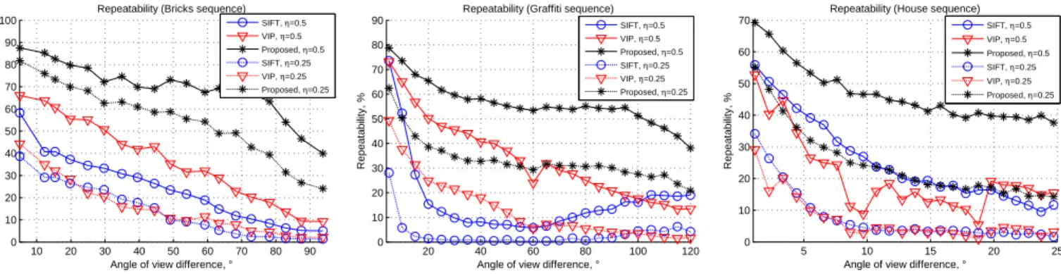
Fig. 4. Repeatability score on synthetic RGBD sequences in function of angle of view difference between reference and test images.
For each test view, we report the repeatability score, equal to the number of repeated keypoints divided by the maximum possible number of repetitions. For the latter we take the maximum number of keypoints detected in one of the two views, excluding those keypoints that fall out of the field of view of any of the two cameras, so that only the surface area present in both views is considered. Moreover, we assume that each keypoint may be repeated at most once (multiple repetitions are not counted: for each 𝐴 only the best matching 𝐵 is considered).
In different variants, this evaluation procedure, originally proposed by Mikolajczyk et al. [7], [8], appears in comparative evaluations of local features, e.g. [6], [10], [11].
We compare the proposed detector to the standard SIFT detector (VLFeat [53] implementation) and to Viewpoint In-variant Patches [30] (original authors’ implementation), which incorporates a keypoint detector that uses the depth map. Three RGBD test sequences are used [1], representing different content, containing significant viewpoint position changes: Bricks (20 images), Graffiti (25 images, re-synthesized from the original Graffiti sequence from [7]) and House (25 images). The repeatability score of each detector is computed for two values of the overlap error threshold 𝜂 = 0.5 and 𝜂 = 0.25. Using two values allows to compare the approaches in two different conditions: the smaller 𝜂 is, the more precisely the keypoints should be repeated. The results of this experiments are shown in Fig. 4.
It can be observed that, for both values of the overlap 𝜂, the proposed detector clearly outperforms the two other approaches. Moreover, even in the tighter condition 𝜂 = 0.25 our proposed detector demonstrates a comparable or better repeatability to the two other detectors, even when those are matched using the more tolerant value 𝜂 = 0.5.
It is worth noticing that in this experiment the number of keypoints detected by SIFT and our proposed method remain comparable (vary between 1000 and 2500 depending on the input image), however VIP detects generally more keypoints (up to 5000).
B. Scene recognition using Kinect images
In this section, we analyze the performance of the proposed RGBD detector in a simple scene recognition application which requires repeatable local features. Using Microsoft
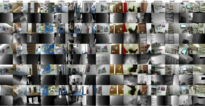
Kinect sensor, we captured 75 RGBD images in 15 different indoor location (5 images per location taken from different positions, but in such a way that the same objects are visible in all the 5 images). The images are shown in Fig. 5. The problem is, e.g., for a mobile robot or a drone, to recognize the location (room) where it is situated, solely using visual sensors data and prior knowledge, i.e., a database of local features representing different locations.
This problem may be reduced to a simple classification task. In order to classify a given image 𝐼 with respect to a set of references ℛ = {(𝐼𝑘, 𝑙𝑘)}𝐾𝑘=1, where 𝑙𝑘 represent the ground
truth class label (i.e., room number), we simply look for an index 𝑘* of an image from ℛ that represents the best match against 𝐼. The best match is the one that maximizes an image similarity score, which is computed as follows.
We detect keypoints in both images and match their cor-responding descriptors. Since the description of detected key-points is out of scope of this paper, we use existing state-of-the-art descriptors presented further in this section. The descriptors are matched testing all descriptor pairs: for each given descriptor from the first image we pick the closest descriptor from the second image. If the number of closely matching descriptors (those that have a distance less than a given matching selectivity threshold 𝑡) is large enough, then the two images are assumed visually similar. Thus, to recognize the location, we select the most similar image and take its label.
Specifically, let 𝑁𝑓 𝑒𝑎𝑡(𝐼) denote the number of features
extracted from image 𝐼 and 𝑁𝑚𝑎𝑡𝑐ℎ𝑒𝑠(𝐼, 𝐼𝑘, 𝑡) the number of
matching descriptor pairs having the inter-descriptor distance less than a threshold 𝑡. Then, the image-level similarity score is given by 𝐽 (𝐼, 𝐼𝑘, 𝑡) = 𝑁𝑚𝑎𝑡𝑐ℎ𝑒𝑠(𝐼, 𝐼𝑘, 𝑡) 𝑁𝑓 𝑒𝑎𝑡(𝐼) + 𝑁𝑓 𝑒𝑎𝑡(𝐼𝑘) − 𝑁𝑚𝑎𝑡𝑐ℎ𝑒𝑠(𝐼, 𝐼𝑘, 𝑡) . (19) The best match with respect to the given set of references ℛ is the one maximizing 𝐽 :
𝑘*(𝐼, 𝑡) = arg max
𝑘 {𝐽 (𝐼, 𝐼𝑘, 𝑡)} . (20)
The label 𝑙𝑘* is then attributed to 𝐼. If the ground truth label
of 𝐼 is equal to 𝑙𝑘*, the image is classified correctly, i.e., the
board boxes casiers carte coffee juice extinguisher coridor entrance livingroom office pictures shelf printer telecom
Fig. 5. Images used for scene recognition task: texture and depth maps of 15 indoor scenes of 5 images acquired with Microsoft Kinect 2 sensor (color image following by depth map in each column). The depth maps are aligned to the texture maps using calibration coefficients carried by the sensor. The images were cropped and subsampled to 720×540 pixels. No other preprocessing (filtering or denoising) is applied.
Differently to the previous experiment, here we involve complete feature extraction pipelines (containing both detector and descriptor). We compare the following local feature ex-traction methods, representing well-known techniques to deal with out-of-plane rotations:
∙ original VIP features [30],
∙ standard SIFT features (VLFeat [53] implementation, referred to as DOG+SIFT),
∙ SIFT descriptors undergoing affine normalization [28], bootstrapped with SIFT keypoints (VLFeat implementa-tion, referred to as DOG+AFFINE),
∙ our proposed detector with standard SIFT descriptors
(referred to as PROPOSED+SIFT),
∙ SIFT descriptors undergoing affine normalization [28],
bootstrapped with our proposed detector (referred to as PROPOSED+AFFINE).
To keep the comparison fair, for all the detectors we keep at most 1000 keypoints with the highest scores (Laplacian response). All input parameters of all the methods keep their default values.
All the descriptors are represented by 128-dimensional numerical vectors. There are two options to measure the inter-descriptor similarity:
1) simple Euclidean norm of inter-descriptor difference taken as a vector;
2) ratio of Euclidean distances to the 1st closest and the 2nd closest descriptor, as proposed in [22].
It is known [22] that in case of standard SIFT descriptors, the second measure allows to preserve better true positive matches when thresholding. However, for descriptors that undergo the affine normalization, the first measure gives higher performance [16]. For each method we simply use
VIP DoG+SIFT Proposed+SIFT DoG+Affine Proposed+Affine 0 0.2 0.4 0.6 0.8 1 Recognition accuracy 57.3% 34.7% 85.3% 49.7% 96.0% 60.6% 97.3% 68.5% 98.7% 71.0% Complete Single ref.
Fig. 6. Accuracy of scene recognition on the images of Fig. 5. The left bars (complete) are computed by matching a query image to all the remaining 74 images in the dataset. In the single-reference classification, instead, each image is classified using a set of 15 randomly selected reference images (one per class). In this case the reported results are the average over 100 repetitions, corresponding standard deviation is displayed.
the option that performs better: the first one is used with DOG+AFFINE and PROPOSED+AFFINE, the second one is used for the rest. Moreover, to have a fair comparison between the tested methods, we perform the experiment for a set of matching selectivity threshold values 𝑡, as there is no reason that different features will perform equally well with the same threshold. For each method we present its best result over all the used values of 𝑡.
Similarly to [32], we first match all the images against each other computing confusion matrices. This allows to classify each given image with respect to all the others, so that the reference set ℛ is different for each input and consists of 74 remaining images. The portion of correctly classified images per method in this setting is reported in Fig. 6 (left bars, referred to as complete). Then we switch to a more practical
Fig. 7. Raw (putative) feature matches between two RGBD images from Boardscene obtained with affine-covariant descriptors on top 1000 keypoints in each image. Left: SIFT detector (243 matches), right: the proposed detector (419 matches).
scenario. We randomly select a single image per location, forming a reference set ℛ of 15 images, and then classify all the remaining images with respect to the given reference set. The obtained recognition accuracy is also shown in Fig. 6 (right bars, referred to as single-ref ). In order to avoid the influence of the random reference selection, we repeat the experiment 100 times.
Our proposed detector achieves a higher recognition accu-racy in both the experiments. Affine normalization compen-sates the perspective distortions on the descriptor computa-tion stage, yielding improved performance compared to the unnormalized SIFT descriptors. For qualitative comparison, an additional illustration of matching using these descriptors is given in Fig. 7: keypoints detected with the proposed detector generally provide more consistent and regular cor-respondences. Moreover, in spite of the noise present in depth maps and their incompleteness (some areas have undefined depth, which is a common problem of infrared depth sensors), our proposed approach is able to detect repeatable keypoints. However, the degraded depth map quality is probably the reason for the limited performance of VIP.
In this experiment we also report that the keypoint detection time taken by our proposed detector averaged over all the 75 images is about 0.42 seconds3. It is nearly half of the
average computation time of VLFeat SIFT detector, which is implemented in a single thread on CPU, but uses vectorial processor instructions in order to speed up the processing.
VI. CONCLUSION
In this paper we have proposed a multiscale representation and a keypoint detector for RGBD images. First, we have proven that the proposed multiscale representation is causal in the image plane, i.e., it engenders a scale space. Second,
3Run on a Windows 7 machine with 12-core 3.5 GHz Intel Xeon CPU, 16
GB RAM and NVidia Quadro K620 graphic card.
since the generation of this scale space corresponds to an approximated diffusion along the surfaces of the scene, the resulting keypoints have a higher stability to large viewpoint changes than conventional, isotropic scale spaces. Finally, the proposed diffusion scheme is numerically stable, linear in the input texture image, and can be efficiently computed on GPU using OpenGL.
These properties have been leveraged to design a novel multiscale detector, which offers a significant gain in terms of keypoint repeatability with respect to viewpoint position changes, both on synthetic and real RGBD images, in a computational time comparable to alternative conventional detectors such as SIFT. Future work will concentrate on completing the feature extraction pipeline with an efficient local description of RGBD content adapted to the proposed detector.
REFERENCES
[1] M. Karpushin, G. Valenzise, and F. Dufaux, “A scale space for tex-ture+depth images based on a discrete Laplacian operator,” in IEEE Intern. Conf. on Multimedia and Expo, Torino, Italy, July 2015. [2] Z. Liu, H. Li, W. Zhou, R. Hong, and Q. Tian, “Uniting keypoints: Local
visual information fusion for large-scale image search,” IEEE Trans. Multimedia, vol. 17, no. 4, pp. 538–548, 2015.
[3] U. L. Altintakan and A. Yazici, “Towards effective image classification using class-specific codebooks and distinctive local features,” IEEE Trans. Multimedia, vol. 17, no. 3, pp. 323–332, 2015.
[4] Y.-G. Jiang, J. Yang, C.-W. Ngo, and A. Hauptmann, “Representations of keypoint-based semantic concept detection: A comprehensive study,” IEEE Trans. Multimedia, vol. 1, no. 12, pp. 42–53, 2010.
[5] A. Redondi, M. Cesana, M. Tagliasacchi, I. Filippini, G. D´an, and V. Fodor, “Cooperative image analysis in visual sensor networks,” Ad Hoc Networks, vol. 28, pp. 38–51, 2015.
[6] F. Fraundorfer and H. Bischof, “A novel performance evaluation method of local detectors on non-planar scenes,” in Proceed. of IEEE Intern. Conf. on Comp. Vision and Pattern Rec., San Diego, USA, May 2005. [7] K. Mikolajczyk and C. Schmid, “A performance evaluation of local descriptors,” IEEE Trans. Pattern Anal. Machine Intell., vol. 27, no. 10, pp. 1615–1630, 2005.
[8] K. Mikolajczyk, T. Tuytelaars, C. Schmid, A. Zisserman, J. Matas, F. Schaffalitzky, T. Kadir, and L. Van Gool, “A comparison of affine region detectors,” Intern. J. of Comp. Vision, vol. 65, no. 1-2, pp. 43– 72, 2005.
[9] P. Moreels and P. Perona, “Evaluation of features detectors and descrip-tors based on 3D objects,” Intern. J. of Comp. Vision, vol. 73, no. 3, pp. 263–284, 2007.
[10] J. Heinly, E. Dunn, and J.-M. Frahm, “Comparative evaluation of binary features,” in Computer Vision–ECCV 2012. Firenze, Italy: Springer, October 2012.
[11] A. Canclini, M. Cesana, A. Redondi, M. Tagliasacchi, J. Ascenso, and R. Cilla, “Evaluation of low-complexity visual feature detectors and descriptors,” in Proceed. of IEEE Intern. Conf. on Dig. Signal Proc., Fira, Santorini, Greece, July 2013.
[12] Y. Guo, M. Bennamoun, F. Sohel, M. Lu, J. Wan, and N. M. Kwok, “A comprehensive performance evaluation of 3D local feature descriptors,” International Journal of Computer Vision, pp. 1–24, 2015.
[13] D. Mukherjee, Q. J. Wu, and G. Wang, “A comparative experimental study of image feature detectors and descriptors,” Machine Vision and Applications, pp. 1–24, 2015.
[14] ISO/IEC JTC 1/SC 29/ WG 11, “CDVS: Requirements,” ISO/IEC, Geneva, MPEG document N11531, July 2010.
[15] ——, “CDVA: Requirements,” ISO/IEC, Valencia, MPEG document N14509, March 2014.
[16] M. Karpushin, G. Valenzise, and F. Dufaux, “Local visual features extraction from texture+depth content based on depth image analysis,” in Proceed. of IEEE Intern. Conf. Image Proc., Paris, France, October 2014.
[17] I. Tosic and K. Berkner, “3D keypoint detection by light field scale-depth space analysis,” in Proceed. of IEEE Intern. Conf. Image Proc., Paris, France, October 2014.
[18] J. Han, L. Shao, D. Xu, and J. Shotton, “Enhanced computer vision with Microsoft Kinect sensor: A review,” IEEE Trans. on Cybernetics, vol. 43, no. 5, pp. 1318–1334, 2013.
[19] H. Gonzalez-Jorge, B. Riveiro, E. Vazquez-Fernandez, J. Mart´ınez-S´anchez, and P. Arias, “Metrological evaluation of Microsoft Kinect and ASUS Xtion sensors,” Measurement, vol. 46, no. 6, pp. 1800–1806, 2013.
[20] M. Karpushin, G. Valenzise, and F. Dufaux, “Improving distinctiveness of BRISK features using depth maps,” in Proceed. of IEEE Intern. Conf. Image Proc., Qu´ebec city, Canada, September 2015.
[21] E. R. do Nascimento, G. L. Oliveira, A. W. Vieira, and M. F. Cam-pos, “On the development of a robust, fast and lightweight keypoint descriptor,” Neurocomputing, vol. 120, pp. 141–155, 2013.
[22] D. G. Lowe, “Distinctive image features from scale-invariant keypoints,” Intern. J. of Comp. Vision, vol. 60, no. 2, pp. 91–110, 2004.
[23] H. Bay, A. Ess, T. Tuytelaars, and L. Van Gool, “Speeded-up robust features (SURF),” Comp. Vision and Image Understanding, vol. 110, no. 3, pp. 346–359, 2008.
[24] S. Leutenegger, M. Chli, and R. Y. Siegwart, “BRISK: Binary robust invariant scalable keypoints,” in Proceed. of IEEE Intern. Conf. on Comp. Vision, Barcelona, Spain, November 2011.
[25] E. Rublee, V. Rabaud, K. Konolige, and G. Bradski, “ORB: an efficient alternative to SIFT or SURF,” in Proceed. of IEEE Intern. Conf. on Comp. Vision, Barcelona, Spain, November 2011.
[26] J.-M. Morel and G. Yu, “ASIFT: A new framework for fully affine invariant image comparison,” SIAM Journal on Imaging Sciences, vol. 2, no. 2, pp. 438–469, 2009.
[27] K. Mikolajczyk and C. Schmid, “An affine invariant interest point detector,” in Computer Vision–ECCV 2002. Springer, 2002, pp. 128– 142.
[28] ——, “Scale & affine invariant interest point detectors,” Intern. J. of Comp. Vision, vol. 60, no. 1, pp. 63–86, 2004.
[29] Y. Pang, W. Li, Y. Yuan, and J. Pan, “Fully affine invariant SURF for image matching,” Neurocomputing, vol. 85, pp. 6–10, 2012.
[30] C. Wu, B. Clipp, X. Li, J.-M. Frahm, and M. Pollefeys, “3D model matching with viewpoint-invariant patches (VIP),” in Proceed. of IEEE Intern. Conf. on Comp. Vision and Pattern Rec., Anchorage, Alaska, USA, June 2008.
[31] A. Zaharescu, E. Boyer, K. Varanasi, and R. Horaud, “Surface feature detection and description with applications to mesh matching,” in Proceed. of IEEE Intern. Conf. on Comp. Vision and Pattern Rec., Miami, USA, June 2009.
[32] N. Werghi, S. Berretti, and A. Del Bimbo, “The Mesh-LBP: a framework for extracting local binary patterns from discrete manifolds,” IEEE Trans. Image Processing, vol. 24, pp. 220–235, 2015.
[33] A. Kovnatsky, M. M. Bronstein, A. M. Bronstein, and R. Kimmel, “Photometric heat kernel signatures,” in Proceed. of 3rd Intern. Conf. on Scale Space and Variational Methods in Computer Vision, Ein-Gedi, Israel, May 2011.
[34] K. Koser and R. Koch, “Perspectively invariant normal features,” in Proceed. of IEEE Intern. Conf. on Comp. Vision, Rio de Janeiro, Brazil, October 2007.
[35] F. Tombari, S. Salti, and L. Di Stefano, “A combined texture-shape descriptor for enhanced 3D feature matching,” in Proceed. of IEEE Intern. Conf. Image Proc., Brussels, Belgium, September 2011. [36] T.-W. R. Lo and J. P. Siebert, “Local feature extraction and matching
on range images: 2.5D SIFT,” Comp. Vision and Image Understanding, vol. 113, no. 12, pp. 1235–1250, 2009.
[37] B. Steder, R. B. Rusu, K. Konolige, and W. Burgard, “Point feature extraction on 3D range scans taking into accountobject boundaries,” in Proceed. of IEEE Intern. Conf. on Rob. and Autom., Shanghai, China, May 2011.
[38] B. Lin, F. Zhao, T. Tamaki, F. Wang, and L. Xiao, “SIPF: Scale invariant point feature for 3D point clouds,” in Proceed. of IEEE Intern. Conf. Image Proc., Qubec City, Canada, October 2015.
[39] J. Weickert, Anisotropic diffusion in image processing. Teubner Stuttgart, 1998, vol. 1.
[40] J. J. Koenderink, “The structure of images,” Biological cybernetics, vol. 50, no. 5, pp. 363–370, 1984.
[41] P. Perona and J. Malik, “Scale-space and edge detection using anisotropic diffusion,” IEEE Trans. Pattern Anal. Machine Intell., vol. 12, no. 7, pp. 629–639, 1990.
[42] G. Sapiro, Geometric partial differential equations and image analysis. Cambridge university press, 2006.
[43] F. Calderero and V. Caselles, “Multiscale analysis for images on rie-mannian manifolds,” SIAM Journal on Imaging Sciences, vol. 7, pp. 1108–1170, 2014.
[44] P. F. Alcantarilla, A. Bartoli, and A. J. Davison, “KAZE features,” in Computer Vision–ECCV 2012. Florence, Italy: Springer, October 2012. [45] S. Wang, H. You, and K. Fu, “BFSIFT: A novel method to find feature matches for SAR image registration,” IEEE Geoscience and Remote Sensing Letters, vol. 9, no. 4, pp. 649–653, 2012.
[46] M. Gobara and D. Suter, “Feature detection with an improved anisotropic filter,” in Computer Vision–ACCV 2006, Hyderabad, India, January 2006. [47] C.-C. Su, L. K. Cormack, and A. C. Bovik, “Color and depth priors in natural images,” IEEE Trans. Image Processing, vol. 22, no. 6, pp. 2259–2274, 2013.
[48] C.-C. Su, A. C. Bovik, and L. K. Cormack, “Natural scene statistics of color and range,” in Proceed. of IEEE Intern. Conf. Image Proc., Brussels, Belgium, 2011.
[49] T. Lindeberg and L. Bretzner, “Real-time scale selection in hybrid multi-scale representations,” pp. 148–163, 2003.
[50] C. Harris and M. Stephens, “A combined corner and edge detector.” in Alvey vision conference, vol. 15, Manchester, UK, 1988, p. 50. [51] M. Agrawal, K. Konolige, and M. R. Blas, “Censure: Center surround
extremas for realtime feature detection and matching,” in Computer Vision–ECCV 2008. Marseille, France: Springer, 2008.
[52] M. Brown and D. G. Lowe, “Invariant features from interest point groups.” in Proceed. of British Machine Vision Conf., Cardiff, UK, September 2002.
[53] A. Vedaldi and B. Fulkerson, “VLFeat: An open and portable library of computer vision algorithms,” in Proceed. of Intern. Conf. on Multimedia, ser. MM ’10, New York, USA, 2010.
Maxim Karpushin received the Master degree in computer science from T´el´ecom ParisTech, France in double diploma program with Novosibirsk State University, Russia (2013) and the Master degree from Novosibirsk State University (2011, cum laude). Now he is a Ph.D. candidate in the Labora-toire Traitement et Communication de l’Information at T´el´ecom ParisTech. His current interests include computer vision and image processing.
Giuseppe Valenzise was born in 1982. He received the Master degree (2007, cum laude) in computer engineering and the Ph.D. degree in electrical en-gineering and computer science (2011), from the Politecnico di Milano, Italy.
From July 2011 to September 2012 he was a post-doc researcher at T´el´ecom ParisTech, Paris, France. He is currently a permanent CNRS researcher with the Laboratoire Traitement et Communication de l’Information at T´el´ecom ParisTech. His research interests include single and multiview video coding, nonnormative tools in video coding standards, multimedia forensics, video quality monitoring, and applications of compressive sensing.
Fr´ed´eric Dufaux received his M.Sc. in physics and Ph.D. in electrical engineering from EPFL in 1990 and 1994 respectively. He has over 20 years of experience in research, previously holding positions at EPFL, Emitall Surveillance, Genimedia, Compaq, Digital Equipment, MIT, and Bell Labs. He has been involved in the standardization of digital video and imaging technologies, participating both in the MPEG and JPEG committees. He is the recipient of two ISO awards for his contributions.
Fr´ed´eric is an IEEE Fellow. He was Vice General Chair of ICIP 2014. He is an elected member of the IEEE Image, Video, and Multidimensional Signal Processing (IVMSP) and Multimedia Signal Processing (MMSP) Technical Committees. He is also the Chair of the EURASIP Special Area Team on Visual Information Processing.
His research interests include image and video coding, distributed video coding, 3D video, high dynamic range imaging, visual quality assessment, video surveillance, privacy protection, image and video analysis, multimedia content search and retrieval, and video transmission over wireless network. He is the author or co-author of more than 120 research publications and holds 17 patents issued or pending.