CC Meets FIPS: A Hybrid Test Methodology for First Order Side Channel Analysis

HAL Id: hal-02413209

https://hal.inria.fr/hal-02413209

Submitted on 16 Dec 2019

HAL is a multi-disciplinary open access

archive for the deposit and dissemination of

sci-entific research documents, whether they are

pub-lished or not. The documents may come from

teaching and research institutions in France or

abroad, or from public or private research centers.

L’archive ouverte pluridisciplinaire HAL, est

destinée au dépôt et à la diffusion de documents

scientifiques de niveau recherche, publiés ou non,

émanant des établissements d’enseignement et de

recherche français ou étrangers, des laboratoires

publics ou privés.

CC Meets FIPS: A Hybrid Test Methodology for First

Order Side Channel Analysis

Debapriya Roy, Shivam Bhasin, Sylvain Guilley, Annelie Heuser, Sikhar

Patranabis, Debdeep Mukhopadhyay

To cite this version:

Debapriya Roy, Shivam Bhasin, Sylvain Guilley, Annelie Heuser, Sikhar Patranabis, et al.. CC

Meets FIPS: A Hybrid Test Methodology for First Order Side Channel Analysis. IEEE

Trans-actions on Computers, Institute of Electrical and Electronics Engineers, 2019, 68 (3), pp.347-361.

�10.1109/TC.2018.2875746�. �hal-02413209�

CC meets FIPS: A Hybrid Test Methodology for

First Order Side Channel Analysis

Debapriya Basu Roy, Shivam Bhasin, Sylvain Guilley, Annelie Heuser, Sikhar Patranabis,

Debdeep Mukhopadhyay

Abstract—Common Criteria (CC) and FIPS 140-3 are two popular side channel testing methodologies. Test Vector Leakage Assessment

Methodology (TVLA), a potential candidate for FIPS, can detect the presence of side-channel information in leakage measurements. However, TVLA results cannot be used to quantify side-channel vulnerability and it is an open problem to derive its relationship with side channel attack success rate (SR), i.e. a common metric for CC. In this paper, we extend the TVLA testing beyond its current scope. Precisely, we derive a concrete relationship between TVLA and signal to noise ratio (SNR). The linking of the two metrics allows direct computation of success rate (SR) from TVLA for given choice of intermediate variable and leakage model and thus unify these popular side channel detection and evaluation metrics. An end-to-end methodology is proposed, which can be easily automated, to derive attack SR starting from TVLA testing. The methodology works under both univariate and multivariate setting and is capable of quantifying any first order leakage. Detailed experiments have been provided using both simulated traces and real traces on SAKURA-GW platform. Additionally, the proposed methodology is benchmarked against previously published attacks on DPA contest v4.0 traces, followed by extension to jitter based countermeasure. The result shows that the proposed methodology provides a quick estimate of SR without performing actual attacks, thus bridging the gap between CC and FIPS.

Index Terms—Side Channel, Evaluation Based Testing, Validation Based Testing, TVLA, NICV

F

1

I

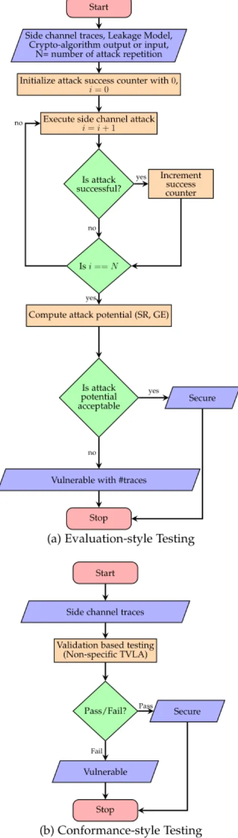
Since the seminal work by Kocher et al. [1], side channels have emerged as a serious threat to implementations of cryptographic algorithms in the past two decades, with the ability to render even mathematically robust cryptographic algorithms vulnerable. A side-channel adversary observes the physical properties of a cryptographic implementation, such as timing, power or electromagnetic emanations, and tries to infer the secret key by modeling a sensitive in-termediate state of the design which depends on these physical properties. Cryptographic designs must, therefore, provide security guarantees against such threats. In this context, efficient validation and evaluation methodology for testing side channel vulnerability has gathered significant interest in the research community. In particular, there exist today, two popular security certification programs - Common Criteria (CC) [2] and FIPS [3] that recommend crypto-implementations to be secure against side channel attacks. Each of these programs follows two distinct testing method-ologies, namely evaluation-style testing, and conformance-style testing.

1.1 Evaluation-style Testing.

The Common Criteria (CC) certification is a prime example of evaluation-style testing. CC is essentially a set of security

∙ Debapriya Basu Roy, Sikhar Patranabish and Debdeep Mukhopadhyay are

with Secured Embedded Architecture Laboratory (SEAL), IIT Kharagpur.

∙ Shivam Bhasin is with Temasek Laboratories, NTU.

∙ Annelie Heuser is with IRISA/CNRS, Rennes, France.

∙ Sylvain Guilley is with TELECOM-ParisTech, France and Secure-IC

S.A.S., France.

guidelines (ISO-15408) that define a common framework for evaluating cryptographic implementations using a standard set of pre-defined evaluation assurance levels. A typical eval-uation based testing mechanism is shown in Fig. 1(a). From the point of view of detecting side channel vulnerabilities, it recommends evaluating the system against all state-of-the-art attack strategies, with the knowledge of the threat model. The evaluator needs to perform different side channel attacks starting from simple power attacks to higher order differential power attacks with different leakage models. Additionally, each of these attacks is repeated multiple times to compute metrics like success rate (SR). An ever-increasing list of attack strategies, together with a large number of models characterizing different leakage profiles of the device, often renders such a testing methodology cumbersome, costly and limited by the testing expertise available at hand. Additionally, the success of evaluation-style testing methodologies depends strongly on appropriate choices of the leakage models, and an error of judgement in this regard could cause a potentially vulnerable crypto-implementation to pass the test. This makes evaluation style testing mechanisms costly and dependent on lab expertise.

1.2 Conformance-Style Testing.

Unlike CC, FIPS [3] certification is an example of conformance-style testing that uses a cryptographic module validation program (CMVP) to validate target’s compliance with necessary security levels rather than an exact eval-uation of its vulnerability. With respect to side channels, it employs a simplified approach for merely detecting the presence of any leakage, independent of attack methodolo-gies and leakage models. This makes it possible to have structured conformance-style testing methodologies that are

Start

Side channel traces, Leakage Model, Crypto-algorithm output or input,

N= number of attack repetition Initialize attack success counter with0,

𝑖 = 0

Execute side channel attack

𝑖 = 𝑖 + 1 Is attack successful? Increment success counter yes Is𝑖 == 𝑁 no no

Compute attack potential (SR, GE)

yes

Is attack potential

acceptable Secure

yes

Vulnerable with #traces

no

Stop

(a) Evaluation-style Testing

Start

Side channel traces

Validation based testing (Non-specific TVLA)

Pass/Fail? Pass Secure

Vulnerable

Fail

Stop

(b) Conformance-style Testing

Fig. 1: Existing Side Channel Testing Methodologies cost-effective and consistent across different testing labs with varied testing expertise. Fortifications with precise security specifications and test plan coverage have the potential to make this style of testing against side-channel vulnerabilities highly efficient and suitable for wide-scale use. A typical conformance-style testing mechanism is shown in Fig. 1(b).

However, the conformance-style testing mechanism can only detect the presence of side channel vulnerability, it is not capable of quantifying the side channel vulnerability. On the other hand, though evaluation-style testing mechanism has many disadvantages, it can quantify side channel

susceptibil-ity, while also finding application in comparing vulnerability of two designs.

Test Vector Leakage Assessment (TVLA) [4] which was proposed at NIST sponsored NIAT workshop in 2011, is one of the well-known conformance style testing mechanism which has gained popularity among the researchers and especially the practitioners due to its robustness, applicability to different crypto-implementations and easy integrability with the existing testing methodologies. Multiple research papers (e.g. [5]) on side channel attacks have used this tool to show the effectiveness of their proposed attacks and countermeasures. TVLA uses the well known Welch’s t-test. It was proposed as a PASS/FAIL test, which checks if 𝑡-value crosses the pre-defined threshold (proposed as ±4.5 [4]). If the 𝑡-value crosses the threshold, the measurement is considered to carry data dependent information, which could be potentially exploited.

TVLA can be classified into: non-specific and specific [4]. Non-specific TVLA partitions traces on basis of public inputs (usually plaintext). Specific TVLA partitions based on intermediate key-dependent variables and thus can provide intuitions on the source of leakage. It has been shown in [6] that non-specific TVLA outperforms specific TVLA as the number of false positives will be less in case of non-specific TVLA. Both methods are discussed in details in section 2.

Being a conformance style testing, one demerit of TVLA methodology is that, a failed 𝑡-test may or may not lead to successful key extraction. In other words, we can not quantify the side channel vulnerability of a crypto-systems using the results of this 𝑡-test. Quantifying side channel vulnerability requires the knowledge of leakage models and adversary capability. As discussed earlier, evaluation style testing can achieve this objective, albeit with very high cost. In current form, the result of 𝑡-test can not be used for such side channel vulnerability quantification.

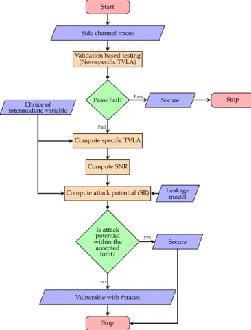
In this paper, we propose a hybrid testing methodology which has the simplicity of conformance-style testing along with the capability of side channel vulnerability quantifi-cation. Our main idea is to use specific TVLA to extract more information regarding the side channel vulnerability of the underlying crypto-implementation. This extracted information can then be expressed in terms of evaluation metrics like signal-to-noise ratio (SNR) and attack success rate (SR). Thus, we first derive the formal relationship be-tween TVLA and SNR. Based on the derived formulation, the hybrid methodology is developed which allows an evaluator to quantify side-channel vulnerability through SR, starting from a basic TVLA analysis. In a nutshell, the proposed methodology bridges the gap between conformance-style and evaluation style testing. We have provided more details on this in section 4. The detailed flow chart of the proposed testing methodology is shown in Fig. 2.

The proposed methodology is also extended to the multivariate setting. As the objective of the proposed testing methodology is to evaluate real products, multivariate analysis can be often required. For instance, often commer-cial smart cards have a built-in clock jitter which causes measurement misalignment. A univariate testing will lead to sub-optimal results, while a multivariate analysis could combine leakages spread over different samples (due to jitter) and evaluate in an optimal manner.

1.3 Related Work

A unified framework to evaluate side channel attack was proposed by Standaert et al. [7]. It puts forward two key metrics success rate (SR) and guessing entropy (GE) as main attack metrics. The success rate of a specific side channel attack is defined as the probability of successful secret key retrieval. In simple mathematical notation, success rate (SR) of a side channel attack (𝐴) is presented as follows:

𝑆𝑅 = 𝑃 𝑟[𝐴(𝐸𝑘0, 𝐿) = 𝑘0] (1)

where 𝑘0is the correct key used in the encryption process

𝐸𝑘0, 𝐿 is the leakage obtained from side channel traces. In

CHES 2012, Fei et al. [8] introduced the notion of confusion coefficient which can be used to compute theoretical success rate of a mono-bit differential power analysis (i.e. difference of mean) given the SNR. This work was further improved and extended to correlation power analysis by Thillard et al. [9]. Fei et al. [10] also extended the initial work on success rate estimation for mono-bit DPA to CPA and beyond.

On the other hand, to simplify the evaluation process, simple and model-agnostic techniques were also developed in parallel. The main technique of this class is the previously mentioned TVLA [4], which was proposed as a FIPS 140-3 candidate. Another simple method to detect point of leakage in a univariate first-order setting was proposed in [11], termed as Normalized Inter Class Variance (NICV). Authors show that NICV is an estimate of SNR and approaches (squared) Pearson’s correlation coefficient in absence of noise. NICV is actually the output of statistical F-test (also known as ANOVA (ANalysis Of VAriance)). Owing to its relationship to SNR, NICV was also used to derive SR for mono-bit DPA using formulation from [8]. In this work, we work on connecting the individual techniques to develop the whole chain. The main missing link in the above techniques is the relationship between TVLA and SNR. By developing that link, we are able to develop a methodology that can be automated end to end to estimate attack SR right from computation of specific TVLA.

1.4 Contribution

The main contributions of this paper are as follows:

∙ SNR of side-channel measurement and TVLA (both

specific and non-specific) are independently developed metrics. We derive the relationship between SNR and TVLA. We formally show that the two metrics are equivalent.

∙ Next, we devise a methodology to estimate the

theoret-ical bounds for the success rate of an attack from the specific TVLA results. This, to our knowledge, is the first attempt to extend specific TVLA results for quantification of side channel vulnerability through SR. The method-ology uses theoretical success rate formulation for CPA by Fei et al. [10]. In other words, the developed method-ology attempts to bridge the gap between conformance and evaluation based testing by setting the following chain: 𝑆𝑝𝑒𝑐𝑖𝑓 𝑖𝑐 𝑇 𝑉 𝐿𝐴 → 𝑆𝑁 𝑅 → 𝑆𝑅.

∙ We also show that using non-specific TVLA to estimate

SNR is impractical, thus motivating the usage of specific TVLA.

∙ The developed methodology is extended to multivariate

setting under first-order leakage setting.

∙ The methodology is practically demonstrated on

unpro-tected AES implementation on an 8-bit microcontroller as well as publicly available traces of protected AES implementation (with accidental leakage) of DPA Con-test v4.0 [12]. We validate the proposed methodology by showing a close match between our predicted SR and the practical SR achieved from the attack published in [13]

The rest of the paper is organized as follows: Section 2 briefly describes the mathematics behind different metrics for validation and evaluation of side channel vulnerabilities. Next, section 3, derives the relationship between Welch’s t-test based TVLA and ANOVA based NICV (and SNR). Section 4 introduces the proposed hybrid design methodology for side channel vulnerability quantification. The proposed formulation is experimentally validated in section 5 followed by application of the hybrid methodology to AES in section 6. The extension of the proposed methodology to multivariate setting is discussed in section 7 followed by final conclusions in section 8.

2

P

In this section, we introduce the notations used throughout the paper, along with brief definitions for the following concepts: TVLA, NICV, SNR, and SR. Finally, the previously proposed relationship between SR and SNR is discussed.

2.1 Notations Used

We denote by 𝑋 and 𝑘 a single plaintext byte and key byte, respectively. We also denote by 𝐿 = 𝑙(𝑋, 𝑘) the normalized

leakage model such that E(𝐿) = 0 and Var(𝐿) = E(𝐿2) = 1.

Finally, we denote by 𝑌 the leakage measurement such that

𝑌 = 𝜖𝐿 + 𝑁 (2)

where 𝜖 is the scaling coefficient and 𝑁 ∼ 𝒩 (0, 𝜎2) is the

noise component, which is independent of 𝑋. Note that the derivations in this paper are based on Eqn. (2). A commonly encountered example for 𝑙(𝑋, 𝑘) is the Hamming weight leakage model on 𝑛 bits, represented as:

𝑙(𝑋, 𝑘) =√2 𝑛 (︁ 𝐻𝑊 (𝑆𝑏𝑜𝑥(𝑋 ⊕ 𝑘)) −𝑛 2 )︁

where 𝑆𝑏𝑜𝑥 denotes the substitution operation. 𝑆𝑏𝑜𝑥(𝑋 ⊕𝐾) is the intermediate variable whose value is mapped to side-channel leakage by the leakage model (HW, for example). With the above notations in place, we present brief definitions for the different side channel metrics used in this paper.

2.2 Signal-to-Noise Ratio

Definition 1. SNR [14, S 4.3.2, page 73] The Signal-to-Noise Ratio (SNR) is defined as:

SNR= Var(E(𝑌 |𝑋))

E(Var(𝑌 |𝑋)) (3)

Lemma 1 (SNR in the case of leakage model (2)).

SNR= 𝜖

2

𝜎2 (4)

Proof 1. Let 𝑥 be a plaintext, and 𝑙 = 𝑙(𝑥, 𝑘). Then E(𝑌 |𝑋 = 𝑥) = E(𝜖𝐿 + 𝑁 |𝐿 = 𝑙) = 𝜖𝑙, by expression of the model (2) and noise independence from the 𝐿. Therefore,

Var(E(𝑌 |𝑋)) = Var(𝜖𝐿) = 𝜖2_{. Besides, E(Var(𝑌 |𝑋)) =}

E(𝜎2_{) = 𝜎}2_{. Hence, SNR =} Var(E(𝑌 |𝑋))

E(Var(𝑌 |𝑋)) = 𝜖2

2.3 Normalized Inter Class Variance

Normalized Inter-Class Variance (NICV) is a technique which was designed to detect relevant point(s) of interest (PoI) in an SCA trace [11]. It has application in side channel trace compression and dimensionality reduction. NICV is based on ANOVA (ANalysis Of VAriance) or F-test [15]. The main advantage of NICV is that it is leakage model agnostic, and can be applied with the knowledge of only plain-text or cipher-text and does not require knowledge of target implementation or secret key.

Definition 2 (NICV [11, Eqn. (4) of Sec. 3.1]). The Normal-ized Inter-Class Variance (NICV) is defined as:

NICV= Var(E(𝑌 |𝑋))

Var(𝑌 ) . (5)

Lemma 2 (NICV in the case of leakage model (2)).

NICV= 1

1 + 𝜎2

𝜖2

. (6)

In particular, 0 ≤ NICV ≤ 1.

Proof 2. The numerator has already been proven to be equal

to 𝜖2. Besides, Var(𝑌 ) = Var(𝜖𝐿) + Var(𝑁 ) = 𝜖2+ 𝜎2_{, by}

independence of 𝑋 and 𝑁 . Hence NICV = Var(_VarE(𝑌 |𝑋))_{(𝑌 )} =

𝜖2 𝜖2_+𝜎2 = 1 1+𝜎2 𝜖2 .

Proposition 1 (Link between NICV and SNR [11, Eqn. (5) of Sec. 3.1]). We have: NICV= ₁ 1 SNR+ 1 and, conversely, SNR= ₁ 1 NICV− 1 . (7) Proof 3. The proof follows from a direct application of the

Lemmas 1 and 2.

2.4 Test Vector Leakage Assessment (TVLA)

Test Vector Leakage Assessment (TVLA) [4] is a direct appli-cation of Welch’s t-test on side channel leakage traces for detection of vulnerabilities. The TVLA methodology can be classified into two different categories: non-specific TVLA and specific TVLA. For both the cases, one must acquire two sets of traces. In case of non-specific TVLA, the first set corresponds to a fixed key and fixed plaintext as input to the cryptographic IP, while the second set contains traces corresponding to the same fixed key and random plaintext. Thereafter a hypothesis testing performed by assuming a null hypothesis that these two sets of traces have identical means and variance. If the null hypothesis is accepted, it signifies that the traces carry no sensitive information. On the other hand, a rejected null hypothesis indicates the presence of exploitable leakage.

More specifically, the non-specific TVLA may be defined mathematically as follows:

Definition 3 (TVLA [4, page 7]). The non-specific TVLA is defined for 𝑄 queries as:

[ TVLA𝑥= = (︃ 1 ∑︀ 𝑞/𝑥𝑞 =𝑥1 ∑︀ 𝑞/𝑥𝑞 =𝑥𝑦𝑞 )︃ − (︂ 1 ∑︀ 𝑞 1 ∑︀ 𝑞 𝑦𝑞 )︂ ⎯ ⎸ ⎸ ⎸ ⎸ ⎸ ⎸ ⎸ ⎸ ⎸ ⎸ ⎸ ⎸ ⎸ ⎷ 1 ∑︀ 𝑞/𝑥𝑞 =𝑥1 (︃ 1 ∑︀ 𝑞/𝑥𝑞 =𝑥1 𝑦2 𝑞− (︃ 1 ∑︀ 𝑞/𝑥𝑞 =𝑥1 𝑦𝑞 )︃2)︃ + 1 ∑︀ 𝑞1 (︃ 1 ∑︀ 𝑞1 𝑦2 𝑞− (︃ 1 ∑︀ 𝑞1 𝑦𝑞 )︃2)︃ (8) where∑︀ 𝑞denotes ∑︀𝑄 𝑞=1and ∑︀ 𝑞/𝑡𝑞=𝑡denotes ∑︀ 1≤𝑞≤𝑄, s.t.𝑡𝑞=𝑡 . We notice that this test is consistent, in that, asymptoti-cally, \ TVLA𝑥−−−−−→ 𝑄→+∞ {︃ +∞ if E(𝑌 |𝑋 = 𝑥) ̸= E(𝑌 ), 0 otherwise.

More precisely, according to the law of large numbers (LLN), we have that: \ TVLA𝑥 ≈ 𝑄→+∞√︀𝑄 E(𝑌 |𝑋 = 𝑥) − E(𝑌 ) √︀Var(𝑌 |𝑋 = 𝑥) + Var(𝑌 ).

We therefore define the asymptotic constant

lim𝑄→+∞√1_𝑄TVLA\𝑥= TVLA𝑥as:

Definition 4. Asymptotic constant for Test Vector Leakage Assessment (TVLA) for Fixed versus Random is:

TVLA𝑥= E(𝑌 |𝑋 = 𝑥) − E(𝑌 )

√︀Var(𝑌 |𝑋) + Var(𝑌 ),

where the fixed plaintext is 𝑥. In this definition, the test is non-specific, since one does not need to know the key. Lemma 3 (TVLA in the case of leakage model (2)).

TVLA𝑥= √𝜖𝑙(𝑥, 𝑘)

𝜖2_{+ 2𝜎}2.

Proof 4. Indeed, we have E(𝑌 ) = 0, hence the result follows. For specific TVLA, knowledge of secret key is required as in this case the traces are partitioned depending upon the value of some intermediate data of crypto-execution [4]. Depending upon the choice of intermediate data, there could be multiple ways to do this partitioning. In [6], the superiority of non-specific TVLA over specific TVLA is established. TVLA is compared with mutual information based analysis techniques in [16] and comparative analysis between them is presented. In [5], authors have focused on the applicability of TVLA. They have extended application of TVLA to higher order attacks. Moreover, they have presented efficient algorithms for on-line computation of TVLA. A modified paired t-test based TVLA methodology is presented in [17]. A recent work [18] shows the limitations of t-test in security evaluation of a higher-order masking scheme, however, for first order evaluation it provides a good starting point.

2.5 SNR and SR

A closed-form expression for DPA and CPA has been derived in [8], [9], [10] that depends on three factors: number of measurements 𝑄, SNR, confusion coefficient vector 𝜅, and

confusion matrices 𝐾, 𝐾**.

Definition 5 (Confusion vector and matrices for CPA [10]).

Let 𝑘𝑐 denote the secret key and 𝑘𝑔𝑖 with 1 ≤ 𝑖 ≤ 2

𝑛−1

a key guess where 𝑘𝑔𝑖̸= 𝑘𝑐, then the confusion vector 𝜅

𝜅= (𝜅(𝑘𝑐, 𝑘𝑔1), . . . , 𝜅(𝑘𝑐, 𝑘𝑔2𝑛−1) 𝑇 𝐾= ⎛ ⎜ ⎝ 𝜅(𝑘𝑐, 𝑘𝑔1, 𝑘𝑔1) 𝜅(𝑘𝑐, 𝑘𝑔1, 𝑘𝑔2) · · · 𝜅(𝑘𝑐, 𝑘𝑔1, 𝑘𝑔2𝑛 −1) .. . ... . .. ... 𝜅(𝑘𝑐, 𝑘𝑔2𝑛 −1, 𝑘𝑔1) 𝜅(𝑘𝑐, 𝑘𝑔2𝑛 −1, 𝑘𝑔2) · · · 𝜅(𝑘𝑐, 𝑘𝑔2𝑛 −1, 𝑘𝑔2𝑛 −1) ⎞ ⎟ ⎠ 𝐾**= ⎛ ⎜ ⎝ 𝜅**_(𝑘 𝑐, 𝑘𝑔1, 𝑘𝑔1) 𝜅 **_(𝑘 𝑐, 𝑘𝑔1, 𝑘𝑔2) · · · 𝜅 **_(𝑘 𝑐, 𝑘𝑔1, 𝑘𝑔2𝑛 −1) .. . ... . .. ... 𝜅**_(𝑘 𝑐, 𝑘𝑔2𝑛 −1, 𝑘𝑔1) 𝜅 **_(𝑘 𝑐, 𝑘𝑔2𝑛 −1, 𝑘𝑔2) · · · 𝜅 **_(𝑘 𝑐, 𝑘𝑔2𝑛 −1, 𝑘𝑔2𝑛 −1) ⎞ ⎟ ⎠ with 𝜅(𝑘𝑐, 𝑘𝑔) = 𝐸((𝑙(𝑋, 𝑘𝑐) − 𝑙(𝑋, 𝑘𝑔))2) 𝜅(𝑘𝑐, 𝑘𝑔𝑖, 𝑘𝑔𝑗) = 𝐸((𝑙(𝑋, 𝑘𝑐) − 𝑙(𝑋, 𝑘𝑔𝑖)(𝑙(𝑋, 𝑘𝑐) − 𝑙(𝑋, 𝑘𝑔𝑗)) 𝜅**(𝑘𝑐, 𝑘𝑔𝑖, 𝑘𝑔𝑗) = 4𝐸((𝑙(𝑋, 𝑘𝑐) − 𝐸(𝑙(𝑋, 𝑘𝑐)))2 (𝑙(𝑋, 𝑘𝑐) − 𝑙(𝑋, 𝑘𝑔𝑖))(𝑙(𝑋, 𝑘𝑐) − 𝑙(𝑋, 𝑘𝑔𝑗))).

Remark 1. In case of no-weak keys 𝜅, 𝐾, 𝐾** are not key

dependent and thus can be determined without knowing

the correct key by setting w.l.o.g 𝑘𝑐= 0.

Now, considering a leakage model as in Eqn. (2), the theoretical success rate is given by

SR= Φ[𝐾+(𝜖

2𝜎)2(𝐾**−𝜅𝜅𝑇)](√︀𝑄

𝜖

2𝜎𝜅) (9)

where Φ[𝐶](𝜇) is the cumulative distributive function of the

multivariate normal distribution with mean vector 𝜇 and

covariance 𝐶. Now as SNR = _𝜎𝜖22 a direct relation between

SNR and SR is given by SR= Φ[𝐾+(1 4)SNR(𝐾**−𝜅𝜅𝑇)](√︀𝑄 1 2 √ SNR𝜅). (10)

Remark 2. The formula of the theoretical success rate in [9] should yield equivalent results. The main difference between [9] and [10] is the normalization of the confusion coefficient(s). Both works are extension of the mono-bit case for DPA introduced in [8]. A further extension to masked implementations has been given in [19], however, since this work targets only first order leakage, masking and higher order attacks remain out of scope.

Note that, Eqn. (9) and Eqn. (10) hold for Eqn. (2) and thus assume that 𝑙(𝑋, 𝑘) is known. However, which has not been mentioned in previous works, is that in a practical scenario one may use an approximation of 𝑙(𝑋, 𝑘) (e.g., 𝐻𝑊 (𝑆𝑏𝑜𝑥(𝑋 ⊕ 𝑘)). This approximation may influence the goodness of the estimation of the theoretical SR in two different ways. First, it may influence the values of

𝜅, 𝐾, 𝐾** _{as the approximation may not have the same}

(less or more) “distinguishing ability” as 𝑙(𝑋, 𝑘). Second, the error made in the approximation of 𝑙(𝑋, 𝑘) introduces additional noise (epistemic noise from the leakage model) which is not captured when estimating the SNR on the traces. From the previous experiments, we observed that the second aspect is more crucial than the first one.

To take a global look at the previous work, NICV is shown directly related with the SNR, which in turn is a main input for computing the minimum number of side channel traces required for performing successful CPA. However, no such

formulation exist in case of specific or non-specific TVLA. In the subsequent section, we will establish the relationship between specific TVLA and SNR so that we can extend the testing mechanism of conformance-style testing.

3

L

B

NICV, SNR

TVLA

3.1 Motivation

Conformance based testing using TVLA is gaining popularity due to its simplicity and ease of computation, but it fails to quantify side channel vulnerability. On the other hand, the evaluation based testing mechanism is highly expensive and lab expertise dependent, but is capable of performing such quantification. In this work, we develop a hybrid methodology which provides the simplicity of conformance style testing mechanism and is able to quantify side channel vulnerability as well. We use specific TVLA to extract more information regarding the side channel vulnerability of the underlying crypto-implementation.

As shown in section 2.5, a series of works have already established closed relation between SNR and SR [8], [9], [10]. Further, this relationship for higher-order attacks tar-geting protected implementations was established in [19]. In this paper, we first establish closed form relation between specific TVLA, SNR and NICV, enabling the computation chain 𝑆𝑝𝑒𝑐𝑖𝑓 𝑖𝑐 𝑇 𝑉 𝐿𝐴 → 𝑆𝑁 𝑅 → 𝑆𝑅. Deriving such relation helps establishing a link between the validation and evaluation style testing, which is the main contribution of this work. We further develop a hybrid testing mechanism combining features of validation and evaluation style testing.

3.2 Linking TVLA and NICV

We follow the same methodology as TVLA i.e. dividing data into two groups followed by application of NICV (and SNR) to it. Let us assume that an adversary has collected 𝑛 number of side channel traces. The entire set of side channel traces is designated as 𝑌 and individual side channel trace is denoted

as 𝑌𝑖, where 𝑖 ∈ [1, 𝑛] is the index of the corresponding

side channel trace. Next following the TVLA approach, the

traces are partitioned into two groups: 𝑌𝐺1and 𝑌𝐺2, having

cardinality 𝑛1 and 𝑛2 (𝑛 = 𝑛1 + 𝑛2) respectively. Mean

and variance of group 𝑌𝐺1 and group 𝑌𝐺2 are denoted

by 𝜇1, 𝜎21 and 𝜇2, 𝜎22 respectively. Moreover, mean and

variance of the entire set 𝑌 are denoted as 𝜇 and 𝜎2. The

objective is to derive the relationship between TVLA and NICV metric. Since we are dealing with only two groups, the

corresponding two groups NICV is denoted as NICV2. This

Theorem 1. Consider two groups of side channel traces 𝑌𝐺1

and 𝑌𝐺2with cardinality 𝑛1and 𝑛2. The computation of

TVLA and NICV2on these two groups are related by the

following formula NICV2= 1 𝑛 TVLA2+ 𝑛 𝐶(𝜎 2 1− 𝜎22) (︃ 1 𝑛2 − 1 𝑛1 )︃ + 1 (11) where 𝐶 =(︀𝜇2 1− 𝜇22 )︀2 .

Proof 5. From Eqn. (5) we can write NICV2as below:

NICV2= 1 𝑛 2 ∑︀ 𝑖=1 𝑛𝑖(𝜇𝑖− 𝜇)2 1 𝑛 𝑛 ∑︀ 𝑖=1 (𝑌𝑖− 𝜇)2 (12)

From Eqn. (8) we can write TVLA as follows:

TVLA= √︁𝜇1− 𝜇2 𝜎2 1 𝑛1 + 𝜎2 2 𝑛2 TVLA2= (𝜇1− 𝜇2) 2 𝜎2 1 𝑛1 + 𝜎2 2 𝑛2 = _𝜎2 𝐶 1 𝑛1 + 𝜎2 2 𝑛2 , (13)

where 𝐶 = (𝜇1− 𝜇2)2. Now we will consider only the

numerator part of the NICV2formulation which is

1 𝑛 2 ∑︁ 𝑖=1 𝑛𝑖(𝜇𝑖− 𝜇)2 = 1 𝑛 (︂ 𝑛1 (︂ 𝜇1− 𝑛1𝜇1+ 𝑛2𝜇2 𝑛 )︂2 + 𝑛2 (︂ 𝜇2− 𝑛1𝜇1+ 𝑛2𝜇2 𝑛 )︂2)︂ = 1 𝑛 (︃ 𝑛1𝑛22 𝑛2 (𝜇1− 𝜇2) 2₊𝑛21𝑛2 𝑛2 (𝜇1− 𝜇2) 2 )︃ =𝑛1𝑛2(𝑛1+ 𝑛2) 𝑛3 𝐶 =𝑛1𝑛2 𝑛2 𝐶. (14)

Next we will consider the denominator part of the NICV computation which is as follows:

1 𝑛 𝑛 ∑︁ 𝑖=1 (𝑌𝑖− 𝜇)2 = 1 𝑛 𝑛 ∑︁ 𝑖=1 (︃ 𝑌_𝑖2−2𝑌𝑖(𝑛1𝜇1+ 𝑛2𝜇2) 𝑛 + (𝑛1𝜇1+ 𝑛2𝜇2)2 𝑛2 )︃ = 1 𝑛 ∑︁ 𝑌𝑖∈𝑌𝐺1 (︂ 𝑌𝑖2− 2𝑌𝑖(𝑛1𝜇1+ 𝑛2𝜇2) 𝑛 )︂ +1 𝑛 ∑︁ 𝑌𝑖∈𝑌𝐺2 (︂ 𝑌_𝑖2−2𝑌𝑖(𝑛1𝜇1+ 𝑛2𝜇2) 𝑛 )︂ +(𝑛1𝜇1+ 𝑛2𝜇2) 2 𝑛2 = 1 𝑛 ∑︁ 𝑌𝑖∈𝑌𝐺1 (︂ 𝑌2 𝑖 − 2𝑌𝑖𝜇1+ 𝜇21+ (︂_2𝑌 𝑖𝑛2(𝜇1− 𝜇2) 𝑛 − 𝜇 2 1 )︂)︂ +1 𝑛 ∑︁ 𝑌𝑖∈𝑌𝐺2 (︂ 𝑌_𝑖2− 2𝑌𝑖𝜇2+ 𝜇22+ (︂_2𝑌 𝑖𝑛1(𝜇2− 𝜇1) 𝑛 − 𝜇 2 2 )︂)︂ +(𝑛1𝜇1+ 𝑛2𝜇2) 2 𝑛2 =𝑛1 𝑛𝜎 2 1+ 𝑛2 𝑛𝜎 2 2+ 𝑛1𝑛2 𝑛2 𝐶. (15)

We can now combine Eqn. (12), (13), (14) and (15) to achieve the desired formulation

NICV2= 𝑛1𝑛2 𝑛2 𝐶 𝑛1 𝑛𝜎12+𝑛𝑛2𝜎22+𝑛𝑛1𝑛22𝐶 = 𝐶 𝑛(︁𝜎21 𝑛1 + 𝜎2 2 𝑛2 + 𝜎 2 1 (︁ 1 𝑛2 − 1 𝑛1 )︁ + 𝜎2 2 (︁ 1 𝑛1 − 1 𝑛2 )︁)︁ + 𝐶 = 1 𝑛 𝜎2 1 𝑛1 +𝜎 2 2 𝑛2 𝐶 + 𝑛 𝐶(𝜎 2 1− 𝜎22) (︃ 1 𝑛2 − 1 𝑛1 )︃ + 1 .

Thus we can write NICV2as

NICV2= 1 𝑛 TVLA2+ 𝑛 𝐶(𝜎 2 1− 𝜎22) (︃ 1 𝑛2 − 1 𝑛1 )︃ + 1 .

Corollary 1. If both the group have the same number of side

channel traces (𝑛1= 𝑛2= 𝑛₂), Eqn. (11) transforms into

NICV2=

1 𝑛

TVLA2+ 1

. (16)

Remark 3. It must be noticed that TVLA needs to be evaluated for a finite number of traces (𝑛), otherwise

it diverges to +∞. However, TVLA2/𝑛 tends to a finite

value when 𝑛 tends to +∞, which bounds the value of

NICV ∈[0, 1].

3.3 Generalizing the NICV Computation

The relationship between TVLA and NICV2(2-class NICV)

was derived previously. However, the general application of NICV (or SNR) is not restricted to two classes. In this

section, the relation between TVLA is extended from NICV2

to a generic k-class NICV (NICV𝑘).

Let us now assume that 𝑛 number of side channel traces

can be partitioned into 𝑘 number of groups where 𝑖𝑡ℎgroup

contains 𝑛𝑖number of traces. A generic example in case of

ciphers like AES, where byte-wise computation is performed

and the desired value of 𝑘 is 256. NICV𝑘 can be directly

computed from NICV2by following an iterative approach.

For the derived 𝑘 groups, 𝑘 different NICV2 is performed

and the results are combined as follows:

∙ ∀𝑖 ∈ Z𝑘, create two groups: the first group contains

the side channel traces with particular byte of the plain-text equal to 𝑖, the other group will contain the side channel traces with that particular byte value not equal to 𝑖. The means of these two groups are denoted

as 𝜇𝑖 and 𝜇𝑖 respectively. Similarly, we denote the

cardinality of these two groups as 𝑛𝑖and 𝑛𝑖= 𝑛 − 𝑛𝑖.

∙ Compute NICV2 for each of these two groups. We

denote this as NICV𝑖2.

Theorem 2. The computations of NICV𝑘 and 𝑁 𝐼𝐶𝑉2 are

related with the following formula

NICV𝑘= 𝑘 ∑︁ 𝑖=1 NICV𝑖₂− 𝑘 ∑︀ 𝑖=1 𝑛2 𝑖 𝑛𝑛𝑖(𝜇𝑖− 𝜇) 2 1 𝑛 𝑛 ∑︀ 𝑗=1 (𝑌𝑗− 𝜇)2 . (17)

Proof 6. From Eqn. (12), we can compute NICV𝑖2as below

NICV𝑖₂= 1 𝑛 (︁ 𝑛𝑖(𝜇𝑖− 𝜇)2+ (𝑛 − 𝑛𝑖) (𝜇𝑖− 𝜇)2 )︁ 1 𝑛 𝑛 ∑︀ 𝑗=1 (𝑌𝑗− 𝜇)2

= 1 𝑛 ⎛ ⎜ ⎝𝑛𝑖(𝜇𝑖− 𝜇) 2 +_𝑛−𝑛1 𝑖 ⎛ ⎜ ⎝ 𝑛𝑖 𝑗=𝑘 ∑︀ 𝑗=1 𝑛𝑗𝜇𝑗−𝑛𝑛𝑖𝜇𝑖 𝑛 ⎞ ⎟ ⎠ 2⎞ ⎟ ⎠ 1 𝑛 𝑛 ∑︀ 𝑗=1 (𝑌𝑗− 𝜇)2 = 𝑛𝑖 𝑛𝑖 (𝜇𝑖− 𝜇) 2 1 𝑛 𝑛 ∑︀ 𝑗=1 (𝑌𝑗− 𝜇)2 , 𝑤ℎ𝑒𝑟𝑒 𝑛𝑖= 𝑛 − 𝑛𝑖. (18)

Now if we add each NICV𝑖2, we will get the following

relationship 𝑘 ∑︁ 𝑖=1 NICV𝑖₂= 𝑘 ∑︀ 𝑖=1 𝑛𝑖 𝑛𝑖(𝜇𝑖− 𝜇) 2 1 𝑛 𝑛 ∑︀ 𝑗=1 (𝑌𝑗− 𝜇)2 = 𝑘 ∑︀ 𝑖=1 𝑛 𝑛𝑖 𝑛𝑖 𝑛(𝜇𝑖− 𝜇)2 1 𝑛 𝑛 ∑︀ 𝑗=1 (𝑌𝑗− 𝜇)2 = 𝑘 ∑︀ 𝑖=1 (1 + 𝑛𝑖 𝑛𝑖) 𝑛𝑖 𝑛(𝜇𝑖− 𝜇) 2 1 𝑛 𝑛 ∑︀ 𝑗=1 (𝑌𝑗− 𝜇)2 = 𝑘 ∑︀ 𝑖=1 𝑛𝑖 𝑛(𝜇𝑖− 𝜇) 2 1 𝑛 𝑛 ∑︀ 𝑗=1 (𝑌𝑗− 𝜇)2 + 𝑘 ∑︀ 𝑖=1 𝑛2 𝑖 𝑛𝑛𝑖(𝜇𝑖− 𝜇) 2 1 𝑛 𝑛 ∑︀ 𝑗=1 (𝑌𝑗− 𝜇)2 . (19)

From Eqn. (12), we can write NICV𝑘 as follows

NICV𝑘= 𝑘 ∑︀ 𝑖=1 𝑛𝑖 𝑛(𝜇𝑖− 𝜇) 2 1 𝑛 𝑛 ∑︀ 𝑗=1 (𝑌𝑗− 𝜇)2 . (20)

Combining Eqn. (19) and (20), we arrive at the following relation 𝑘 ∑︁ 𝑖=1 NICV𝑖₂= NICV𝑘+ 𝑘 ∑︀ 𝑖=1 𝑛2 𝑖 𝑛𝑛𝑖(𝜇𝑖− 𝜇) 2 1 𝑛 𝑛 ∑︀ 𝑗=1 (𝑌𝑗− 𝜇)2 . (21)

Using the assumption of uniform setting, we presume that each group has same number of side channel traces. Then, Eqn. (19) becomes

𝑘 ∑︁ 𝑖=1 NICV𝑖₂= 1 𝑘 𝑘 ∑︀ 𝑖=1 (𝜇𝑖− 𝜇)2+_{𝑘(𝑘−1)}1 𝑘 ∑︀ 𝑖=1 (𝜇𝑖− 𝜇)2 1 𝑛 𝑛 ∑︀ 𝑗=1 (𝑌𝑗− 𝜇)2 = 𝑘 𝑘−1 1 𝑘 𝑘 ∑︀ 𝑖=1 (𝜇𝑖− 𝜇)2 1 𝑛 𝑛 ∑︀ 𝑗=1 (𝑌𝑗− 𝜇)2 = 𝑘 𝑘 − 1NICV𝑘. (22)

Thus we arrive at the desired formulation

𝑁 𝐼𝐶𝑉𝑘 = 𝑘 − 1 𝑘 𝑘 ∑︁ 𝑖=1 𝑁 𝐼𝐶𝑉2𝑖.

It must be noted that NICV𝑘is actually the generalized

NICV which was introduced in [11].

Corollary 2. If all the 𝑘 groups have same number of side channel traces, then

NICV𝑘 = 𝑘 − 1 𝑘 𝑘 ∑︁ 𝑖=1 NICV𝑖₂. (23)

Once we have computed NICV𝑘, we can easily compute SNR

using Eqn. (7).

3.4 Extension to Non-Specific TVLA

In this part, we establish the relationship between SNR and non-specific TVLA. The first hint of the link between SNR and TVLA was qualitatively discussed in [11]. The formal relationship is derived as follows.

Proposition 2 (Link between SNR and TVLA). The SNR is the variance of the TVLA values in the fixed versus random (or non-specific) setup, the variance is computed over all possible fixed values:

SNR= 2Var(TVLA𝑋)

1 − Var(TVLA𝑋).

Proof 7. As TVLA𝑋 = √𝜖𝑙(𝑥,𝑘)_𝜖2_+2𝜎2, we have: Var(TVLA𝑋) =

𝜖2

𝜖2_+2𝜎2Var(𝐿) =

𝜖2_/𝜎2

2+𝜖2_/𝜎2 =

SNR

2+SNR. From here we can

easily derive SNR = 2Var(TVLA𝑋)

1−Var(TVLA𝑋)

For non-specific TVLA, the traces are partitioned depend-ing upon the entire plaintext value, where one group contains traces with fixed plaintext and other contains traces with random plaintext. If we want to extend our approach to non-specific TVLA to compute SNR, we need to compute TVLA for each plaintext value, which is computationally infeasible. Thus, in the following, we stick to specific TVLA only.

4

P

H

S

C

T

M

4.1 Context

Countermeasures against side-channel attack are advancing every year [20]. Alongside, there are comprehensive evalua-tion methodologies which are also developed [21]. However, conducting a comprehensive and detailed security evaluation can be a time-taking task. Time is a limiting factor for the evaluation process and for the same reason CC evaluations contain time spent for the evaluation as a metric. Some work deal with further simplifying the evaluation process [22].

Most, if not all, real implementations are currently con-sidering basic countermeasures due to the cost of security attached. Thus, evaluation laboratories are still often dealing with unprotected or low-order protected cryptographic im-plementations, which might also suffer from accidental first order leakage. Automotive ECUs are a current example. In such scenarios, a simple testing methodology like TVLA can be a good start. However, it might also be desirable/required to quantify the side channel vulnerability. The methodol-ogy proposed in the following combines the efficiency of conformance-style testing mechanism with the purpose of evaluation style mechanism. We later extend the proposed methodology to a multivariate setting as well.

Start

Side channel traces

Validation based testing (Non-specific TVLA)

Pass/Fail? Pass Secure Stop

Compute specific TVLA

Fail

Choice of intermediate variable

Compute SNR

Compute attack potential (SR) Leakage model Is attack potential within the accepted limit? Secure yes

Vulnerable with #traces

no

Stop

Fig. 2: Proposed Hybrid Side Channel Testing Methodology

4.2 Description of the Proposed Methodology

Side channel analysis is based on a divide and conquer approach. For instance, for an SPN cipher where each 𝑏 × 𝑏 S-box handles 𝑏 bits of the entire key bits, the attack focuses on each of these 𝑏 bit groups separately. In case of AES-128, 𝑏 = 8 which means that the attack is applied on 8-bits or one byte of the secret key, also known as a sub-key. The attack can be repeated 16 times to recover all the key bytes or alternatively key enumeration methods can be applied to derive the full key [23]. The same applies to SNR and NICV. One can compute SNR or NICV byte-wise to zero down the leakage zone of each key byte and apply the attack.

In Fig. 2, we present our methodology to extend the TVLA computation to recover the SNR followed by the computation of the success rate with a given leakage model and intermediate variable. The test starts with a non-specific TVLA test to detect the presence of side channel leakage. If this test fails, we first perform specific TVLA for a chosen intermediate variable. Indeed, it is the intermediate value and leakage model that helps in binding the evaluation and conformance based testing in the proposed methodology.

From specific TVLA, NICV2is computed by Eqn. (11), which

further leads to NICV𝑘by Eqn. (17). NICV𝑘(or just NICV) can

directly provide the SNR by Eqn. (7). Finally, SNR leads to SR for a chosen leakage model (Eqn. (10)). The computation of SR through the proposed methodology is presented in the Algorithm 1. As stated in section 3.4, the methodology cannot be applied to non-specific TVLA due to computational infeasibility.

The proposed hybrid methodology brings in several

Algorithm 1:Computing SNR and SR from TVLA

Input:Side channel traces and corresponding intermediate state

Output: SRfor chosen sub-key

1 for 𝑖 = 0 to 𝑘 do

2 Partition the side channel traces into two groups: 𝐺1and 𝐺2

3 𝐺1: Side channel traces where 𝑗𝑡ℎbyte of the intermediate data

= 𝑖

4 𝐺2: Side channel traces where 𝑗𝑡ℎbyte of the intermediate data

̸= 𝑖

5 Apply TVLA on groups 𝐺1and 𝐺2

6 Compute NICV𝑖

2from the TVLA value by using Eqn. (11)

7 Compute NICV𝑘using Eqn. (17)

8 Compute SNR = ₁1 NICV_𝑘−1 9 Compute SR = Φ_{[𝐾+( 1} 4)SNR(𝐾** −𝜅𝜅𝑇 )]( √ 𝑄1 2 √ SNR𝜅) 10 Return SR

TABLE 1: Comparison between existing and proposed testing methodologies

Features Evaluation Conformance Proposed

Leakage model required √ × √

Intermediate value required √ × √

Vulnerability quantification √ × √

Analytical × √ √

advantages as compared to the two individual approaches (evaluation and conformance). It formally shows that the two approaches are not unrelated and propose a basis to compute one from the other. Moreover, the proposed methodology provides a computation acceleration. In comparison to Fig. 1 (a), Fig. 2 does not have any iterative loop for success rate computation. The acceleration is significant in commercial products, where even unprotected implementations might need millions of traces for an attack, repeated several times for success rate computation. The proposed methodology can compute SR for several leakage models in parallel, without significant additional computation, as the knowledge of leakage model is only needed in step 9 of Algo. 1. Since the leakage model projects the intermediate value to side-channel leakage, several projections can be tested in parallel, based on the attacker profile. The methodology can support a range of leakage models from a generic Hamming weight and identity, which can be erroneous, to profiled leakage model of linear and higher dimensions [24], which will be more precise. As shown later, the proposed methodology can also be applied in a multivariate setting. Nevertheless, if TVLA results are not required, the evaluator can directly compute SNR from the traces and follow the remaining methodology.

As for the disadvantages, the choice of intermediate value is required for specific TVLA computation. However, conformance-style testing does not require any prior knowl-edge of leakage model or intermediate variable. This choice of intermediate value requires expertise on part of the evaluator. From another perspective, it is the knowledge or choice of intermediate value which binds the two approaches together. The proposed methodology takes the intermediate value as an external input from the evaluator for specific TVLA computation and allows the user to be flexible in his choice of leakage model or test several in parallel. All these points are summarised in Tab 1.

0 500 1000 1500 −30 −20 −10 0 10 20 30 Time Sample S p ec ifi c T VL A

(a) Single specific TVLA

0 500 1000 1500 0 0.005 0.01 0.015 0.02 0.025 Time Sample N I C V2

(b) Predicted NICV2 from

plot (a) 0 500 1000 1500 0 0.005 0.01 0.015 0.02 0.025 Time Sample N I C V2

(c) Computed NICV2 from

traces 0 500 1000 1500 −4 −3 −2 −1 0 1 2x 10 −15 Time Sample E rr or (d) Prediction Error in Eqn. (11) ((b) - (c))

Fig. 3: Equivalence of TVLA and NICV2

5

E

V

D

TVLA

NICV R

The derived relation between specific TVLA and SNR (or NICV) is experimentally validated in this section on an AES-128 implementation (without side-channel countermeasures) running on an ATMEGA-8515 smart-card.

5.1 Experimental Setup

The AES design is implemented on a SAKURA-GW plat-form [25]. The SAKURA-GW platplat-form supports communi-cation with ATMEGA-8515 smart-card, which in our case runs an unprotected AES-128. The power measurements are taken using a Tektronix MSO4034B mixed signal oscilloscope with sampling frequency 500 𝑀 𝑆𝑎𝑚𝑝𝑙𝑒𝑠/𝑠𝑒𝑐. Being an unprotected implementation, it is obvious that the AES implementation must have exploitable leakage and its TVLA value should be more than the threshold of 4.5.

5.2 Validation of TVLA and NICV2Relationship

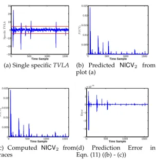
To verify the relationship between TVLA and NICV2 (see

Eqn. (11)) practically, we start with partitioning the traces based on the first-byte value (𝑘 = 256) of the output of round 9 as the intermediate state, following step 1 of Algo. 1.

Next, we compute TVLA and NICV2 from the partitions

again following Algo. 1. The results are shown in Fig. 3. A specific TVLA trace is shown in Fig. 3 (a). Next, the TVLA

trace in Fig. 3 (a) is used to compute NICV2using Eqn. (11)

and shown in Fig. 3 (b). We also compute NICV2from power

measurement as shown in Fig. 3 (c). The error between

predicted and computed NICV2is in the order of 10−15i.e.

negligible and coming from truncation error (Fig. 3 (d)), which confirms Eqn. (11).

5.3 Validation of NICV𝑘and NICV2relationship

Similar validation is also done for Eqn. (17) that relates NICV2

and NICV𝑘. Using the same set of traces and no. of partitions

(𝑘 = 256), we compute NICV𝑘from the traces and predict it

from previously computed NICV2. The results are shown in

Fig. 4. As the computed NICV𝑘(Fig. 4 (a)) follows closely the

predicted NICV𝑘(Fig. 4 (b)), the prediction error (Fig. 4 (c))

also stays in the range of 10−15.

0 500 1000 1500 0 0.2 0.4 0.6 0.8 1 Time Sample Ac tu al N I C Vk

(a) Computed NICV𝑘

0 500 1000 1500 0 0.2 0.4 0.6 0.8 1 Time Sample P re d ic te d N I C V k (b) Predicted NICV𝑘 0 500 1000 1500 −1.5 −1 −0.5 0 0.5 1 1.5 2 2.5x 10 −15 Time Sample E rr or (c) Prediction Error in Eqn. (17) ((a) - (b))

Fig. 4: Prediction of NICV𝑘

6

C

S

: A

AES

The equivalence of TVLA and SNR was theoretically derived and experimentally verified in the previous sections. The step by step procedure to compute SNR (and SR) from the specific TVLA value was presented in Algo. 1. In this section, we focus on the application of these relations towards testing AES in three different settings. First results are shown on simulated power traces, followed by application of the evaluation methodology on actual power traces acquired from unprotected AES implementation running on the same ATMEGA-8515 smart-card which was used in section 5. Finally, the methodology is tested on publicly available DPA Contest v4.0 traces corresponding to a protected AES-256 implementation with some first order leakage.

6.1 Under Simulated Setting

Simulated traces are generated for an 8−bit microcontroller, assuming perfect Hamming weight leakage and added zero

mean Gaussian noise (𝒩 (0, 𝜎2)), where 𝜎2 _{denotes the}

variance of the noise distribution. The side channel trace can be represented as 𝑌 = 𝐻𝑊 (𝑣) + 𝒩 , where 𝑣 is the chosen intermediate value, which in this case is first 8-bits of round 9 output. We have generated side channel traces for different SNR values ranging from 0.03 to 2.

0 0.5 1 1.5 2 0 100 200 300 400 500 600 SNR

#traces for success rate 80%

Practical Theoretical

Fig. 5: Estimation of Number of Traces to Reach 80% SR For Theoretical SR and Practical SR for different SNRs

Next, we directly apply Algo. 1 to first derive SNR and then Eqn. (10) to estimate the number of traces required to achieve 80% SR. A practical CPA attack is also performed

repeatedly on the set of the simulated traces to compute the number of traces required to achieve 80% SR. The corresponding result is shown in Fig. 5, which shows a very close match between the theoretical and practical evaluation. It can be observed that under perfect HW model as-sumption, the estimated theoretical estimation and practical computation fits quite closely. A minor overshoot for prac-tical SR is seen for high SNR (> 0.5). This overshoot is an approximation glitch in the theoretical formulation under central limit theorem and law of large numbers, which needs few dozen traces to converge. Otherwise, the approximation overshoot remains constant even for extremely high SNR (tested up to SNR=20). The overshoot can be seen in real traces as well for high SNR scenarios in the next subsection.

0 20 40 60 80 100 −2 0 2 4 6 8 10x 10 −3 Sampling Points

Power Value (Watt)

p 1 p 2 number of traces/30 0 2 4 6 8 10 SR 0 0.2 0.4 0.6 0.8 1 Theoretical (SNR=0.73) Practical (SNR=0.73) Theoretical (SNR=0.16) Practical (SNR=0.16)

(a) sample point𝑝1

number of traces/30 0 2 4 6 8 10 SR 0 0.2 0.4 0.6 0.8 1 Theoretical (SNR=0.72) Practical (SNR=0.72) Theoretical (SNR=0.14) Practical (SNR=0.14) (b) sample point𝑝2

Fig. 6: Comparison Between Theoretical SR and Practical SR for different SNRs using Hamming weight model at different sample points

6.2 On Real Power Traces

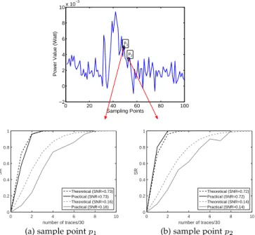
The experimental setup for the acquisition of power traces is equivalent to the one described in section 5.1. Further white Gaussian noise is added to experiment in low-SNR scenarios. The experiments were performed with 20,000 traces. For practical SR, a CPA was mounted on a randomly chosen set of 300 traces (from those 20000), repeated 50 times. Following Algo. 1 and assuming that the ATMEGA-8515 smart-card on the SAKURA-GW board leaks in HW model, we generate plots for estimated theoretical success rate.

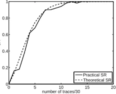
The results are shown in Fig. 6 for two distinct points

𝑝1 and 𝑝2 on the trace. We compute the practical SR and

theoretical SR in the interval of 30 traces. The x-axis in the Fig. 6 denotes the number of such intervals (which is equal to number of traces/30) and the y-axis denotes the corresponding SR value. As we can see, in the low SNR scenario, there is a gap between theoretical SR and practical SR which is due to the improper leakage model.

Finding a device with perfect HW leakage model is a

very strong assumption. The two distinct points: 𝑝1and 𝑝2

are chosen as such that one point has leakage very close to

1 2 3 4 5 6 7 8 1 2 3 4 5 6 7 8 9 10x 10 −4 bit position weightage value

(a) sample point𝑝1with

imperfect HW leakage model

1 2 3 4 5 6 7 8 5 6 7 x 10−4 bit position weightage value

(b) sample point𝑝2which is more close

to HW leakage model

Fig. 7: Sample points with perfect and imperfect HW leakage model

HW model while the other deviates from the model. More

specifically, the sample point 𝑝2has a leakage model closer

to HW model, whereas the sample point 𝑝1has a leakage

model which deviates significantly from the HW model. A closer estimation to the actual model is computed using profiling based on stochastic modeling [24] of leakage into

9 dimensions as Σ8𝑖=1𝛽𝑖𝑣𝑖. The 𝛽 weights of different points

are shown in Fig. 7. Fig. 7(a) shows that in case of point

𝑝1, the leakage model deviates from HW model, whereas

Fig. 7(b) shows that leakage model of point 𝑝2stays close

to HW model. Referring back to Fig. 6, when the SNR is

high, the practical SR for both sampling point 𝑝1 and 𝑝2

closely matches the theoretical prediction. However, as the SNR reduces, the deviation between theoretical and practical SR increases. This deviation is even worse when the model is imperfect (see Fig. 6(a)).

number of traces/30 0 2 4 6 8 10 SR 0 0.2 0.4 0.6 0.8 1 Theoretical (SNR=0.73) Practical (SNR=0.73) Theoretical (SNR=0.16) Practical (SNR=0.16)

(a) sample point𝑝1

number of traces/30 0 2 4 6 8 10 SR 0 0.2 0.4 0.6 0.8 1 Theoretical (SNR=0.72) Practical (SNR=0.72) Theoretical (SNR=0.14) Practical (SNR=0.14) (b) sample point𝑝2

Fig. 8: Comparison Between Theoretical SR and Practical SR for different SNRs using first order stochastic model at different sample points

We repeat the experiments by taking the actual model

into the account and re-running Algo. 11. Precisely it is only

the last step of Algo. 1 which is affected by the leakage model as stated in Eqn. (10). The results are shown in Fig. 8. Again under high SNR, the practical attack results match with the theoretical estimation. However, by taking the correct leakage model into the account, the theoretical estimation of SR and

practical SR also matches closely for sample point 𝑝1(with

imperfect HW leakage model) and sample point 𝑝2 (with

leakage model close to HW leakage model). This match is due to the application of correct leakage model in Algo. 1 which confirms the importance of leakage modeling in a side channel attack. From the methodology aspect, it shows that the better profiled the model is, the more realistic prediction 1. The computation of SR using HW model and stochastic modeling can be executed in parallel.

of SR can be made from the TVLA results. Nevertheless, the evaluator can test several leakage models in parallel at negligible computation overhead.

0 5 10 15 20 0 0.2 0.4 0.6 0.8 1 SR number of traces/30 Practical SR Theoretical SR

Fig. 9: Comparison Between Theoretical SR and Practical SR on DPA Contest v4.0 Traces

6.3 First Order Protected Implementation with Leakage:

DPA Contest v4.0 Traces

Till now, we have discussed the application of the proposed methodology on the unprotected implementations. The proposed hybrid testing methodology can be also applied to the flawed first order protected implementation which exhibits first order leakages due to inefficient implementation or glitches inside the circuits. The side channel traces used in DPA Contest v4.0 [12] is an example of such scenarios. The AES-256 implementation used in DPA Contest v4.0 is based on rotating S-Box making scheme. However, it was shown in [13] that the implementation exhibits univariate first order leakage. Precisely, the attack in [13] exploits the accidental leakage on a single bit when the round 0 key addition result is overwritten by the round 1 Sbox output. The leakage is exploited over a single bit and denoted as (((𝑥 ⊕ 𝑘) ⊕ 𝑆(𝑥 ⊕ 𝑘))&1) (& is logical AND function). In the following, we first compute the practical SR for the attack published in [13], on the available traces with this model to use it as a benchmark. Next, the proposed methodology is applied to predict the SR from specific TVLA testing using the same leakage model.

The practical and theoretical SR are shown in Fig. 9. As shown in Fig. 9, the values of practical and theoretical SR matches very closely which in turn proves the efficiency of the proposed methodology. (((𝑥 ⊕ 𝑘) ⊕ 𝑆(𝑥 ⊕ 𝑘))&1) is used as a intermediate value and the applied leakage model is identity, i.e. specific TVLA and thus SNR are computed for a single bit of model.

7

M

A

Traditionally, multivariate side channel analysis is applied for higher order attacks where leakages from multiple points are combined. Multivariate analysis can be useful even in a first order leakage context because an adversary can retrieve the key much earlier if he combines multiple leakage points in an optimal manner. A relevant scenario where such analysis can be useful is a real industrial product with clock jitter that leads to side-channel measurement misalignment. The leakage is thus spread over multiple time samples due to the jitter. While a univariate analysis in such scenario might be sub-optimal, a multivariate approach can lead to fair evaluation.

In its current form, TVLA metric can not be applied in multivariate analysis without modifying its formulation. Recently in [18], the limitations of TVLA in detection of multivariate side channel vulnerabilities were addressed in details for higher order analysis. In [5], the authors have focussed on extending TVLA methodology to higher order leakage detection. Consequently, a strategy for applying d-th order d-variate TVLA test is given. A typical application for

such analysis can be a software implementation of 𝑑𝑡ℎorder

masking, where shares are executed sequentially.

Our approach in this section is different from them as we focus on 1st order d-variate TVLA test where 𝑑 denotes the dimension of a single side channel trace. We investigate the extension of proposed methodology for unprotected imple-mentation in the multivariate setting for side-channel vulner-ability quantification. Therefore, the weaknesses pointed out in [18], do not apply to our setting. Moreover, in this section, we try to extend the applicability of TVLA from univariate to multivariate settings to address one of the shortcomings of traditional TVLA [18].

7.1 Proposed Formulation

To obtain SR for multivariate side channel analysis, we can follow two different approaches. We can either compute TVLA on each sample and then combine those values to get the corresponding SR in multivariate settings or combine the different sample points using an optimal dimensionality re-duction formulation to convert the multivariate side channel traces into a single point. For latter, we use the framework of [26]. In particular, the traces 𝑌 arise from a single leakage

model 𝐿, which depends on the correct key 𝑘 = 𝑘*, and

which is taken standard (i.e., E(𝐿) = 0, Var(𝐿) = 1), through the relationship:

𝑌𝑑 = 𝛼𝑑𝐿(𝑘*) + 𝑁𝑑,

where 𝑑 is the dimensionality (1 ≤ 𝑑 ≤ 𝐷).

Remark 4. This equation implies E(𝑌 ) = 0. When computing a t-test, using non-specific or specific, the evaluator also

has to evaluate E(𝑌 |𝑋 = 𝑥0) for a given plaintext (or a

given byte value of the plaintext) 𝑥0. Let’s assume that

E(𝑌 |𝑋 = 𝑥0) = 𝑐 ̸= 0. The condition ̸= 0 is here to avoid

having E(𝑌 ) = E(𝑌 |𝑋 = 𝑥0), in which case the attacker

would conclude the device is secure whereas in practice

it is not (e.g. for a different value of 𝑥′0, we would have

E(𝑌 ) ̸= E(𝑌 |𝑋 = 𝑥′

0)).

In matrix form, for 𝑄 number of side channel traces, we can write the above equation as below:

𝑌𝐷,𝑄= 𝛼𝐷𝐿𝑄(𝑘*) + 𝑁𝐷,

Here 𝛼𝐷 is a non-zero vector of length 𝐷, and can be

calculated as follows [26]:

𝛼𝐷= 𝑌

𝐷_(𝐿𝑄_(𝑘*₎₎𝑇

𝐿𝑄_(𝑘*_)𝐿𝑄_(𝑘*₎𝑇. (24)

We assume that the noise 𝑁𝐷 is multivariate normal, and

we denote by Σ its 𝐷 × 𝐷 covariance matrix. The value of Σ can be computed as below [26]:

Σ = 1

𝑄 − 1(𝑌

With the knowledge of 𝛼𝐷and Σ, we can now calculate the optimal dimensionality reduction formulation which is

(𝛼𝐷)𝑇Σ−1𝑌𝐷,𝑄

(𝛼𝐷₎𝑇_Σ−1_𝛼𝐷 [26].

7.1.1 SNR and TVLA in multivariate settings

To compute the SNR and TVLA in multivariate settings, we propose following pre-processing steps. Hereby 𝑏𝑜𝑙𝑑𝑓 𝑎𝑐𝑒 we denote multivariate trace of dimension 𝐷.

∙ Step 1: Compute Σ,

∙ Step 2: Standardize the measurements, that is: 𝑌

becomes 𝑌′= Σ−1/2_{𝑌 .}

Notice that 𝑌′ = (Σ−1/2_{𝛼)𝐿 + 𝑁}′_{, where 𝑁}′ _{is now an}

isotropic standard noise (all 𝐷 samples of noise are i.i.d., of mean 0 and variance 1). Indeed,

E(𝑁′(𝑁′)T_{) = E(Σ}−1/2_{𝑁 𝑁}T_Σ−1/2₎

= Σ−1/2_{E(𝑁 𝑁}T_)Σ−1/2_{= 𝐼, (26)}

where 𝐼 is the 𝐷 × 𝐷 identity matrix.

On step 2, we can now re-estimate 𝜇′1, as E(𝑌′). For the

sake of clarity, we drop index 1 and 2 in 𝜇 (when it is clear given the context). We see that the optimal dimensionality reduction is (theorem 1 of [26]) (𝜇′₎T_𝑌′ (𝜇′₎T_𝜇′ = ‖𝜇 ′_‖−2 (𝜇′₎T_𝑌′_. (27) Consequently, we can define multivariate SNR and multi-variate TVLA as follow:

SNR= (𝜇′₎T_𝜇′₌ 𝐷 ∑︁ 𝑑=1 (𝜇′ 𝑑)2. (28) TVLA2= 𝐷 ∑︁ 𝑑=1 (𝜇′ 1,𝑑− 𝜇′2,𝑑)2 1 𝑛1 + 1 𝑛2 (29) because 𝜎_1,𝑑′ = 𝜎′ 2,𝑑= 1 (by Eqn. (26)).

Remark 5. This is equal to (up to an irrelevant 1₄

proportion-ality factor) the Hotelling’s T-Square [27]). Indeed, let us

consider that 𝑛1= 𝑛2= 𝑛/2. We have:

TVLA2= 𝐷 ∑︁ 𝑑=1 (𝜇′ 1,𝑑− 𝜇′2,𝑑)2 1 𝑛1 + 1 𝑛2 =1 4𝑛(𝜇1− 𝜇2) T_Σ−1_(𝜇 1− 𝜇2). (30)

The definition of multivariate SNR (Eqn. (28)) and multivariate TVLA (Eqn. (29)) remains consistent with the dimensionality reduction (Eqn. (27)). Namely, we have: Proposition 3. The application of univariate SNR (resp TVLA)

of reduced trace (Eqn. (27)) yields multivariate SNR (Eqn. (28)) (resp. multivariate TVLA (Eqn. (29))).

Proof 8. After dimensionality reduction, we get:

𝑌′′= 𝐿 + 1

𝜇𝑇_Σ−1_𝜇𝜇

′𝑇_𝑁′_.

For the SNR, we thus have:

∙ signal: Var(𝐿) = 1; ∙ noise: 1 (𝜇𝑇_Σ−1_𝜇)2Var(𝜇 ′𝑇_𝑁′_{) =} 1 𝜇𝑇_Σ−1_𝜇. (31)

Hence SNR is 𝜇𝑇Σ−1_{𝜇, which is equal to Eqn. (28).}

Regarding TVLA, we will assume that E(𝑌 ) = 𝜇1= 0,

and E(𝑌 |𝑋 = 𝑥0) = 𝜇2= 𝑐𝜇. Hence, after

dimensional-ity reduction (Eqn. (27)), one gets

∙ reduced average for random plaintext: 0,

∙ reduced average for fixed plaintext = 𝑥0: 𝑐,

∙ reduced noise has variance (Eqn. (31)).

Hence the univariate (squared) TVLA on reduced traces is

𝑐2(𝜇𝑇_Σ−1_𝜇).

Now, the multivariate (squared) TVLA (Eqn. (29)) is (using Hotteling formula (Eqn. (30))):

1

4𝑛(0 − 𝑐𝜇)

𝑇_Σ−1_{(0 − 𝑐𝜇),}

which also match with the TVLA expression obtained after dimensionality reduction. It must be noted that this formulation is applicable to both specific and non-specific TVLA test.

7.2 Experimental Results

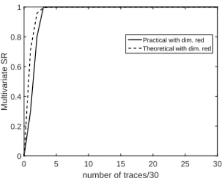
The multivariate setting of the proposed methodology is now experimentally validated on real power traces of an unprotected AES-128 (same as section 6.2). We first apply optimal dimension reduction on the acquired traces to project the multivariate leakage to a single point. As shown in Prop. 3 multivariate SNR computed on the multivariate traces is equivalent to the univariate SNR computed on the dimension reduced traces. Hence, we can use our proposed methodology for univariate traces on the dimension reduced traces and can compute the theoretical SR and practical SR (see Fig. 10). Firstly, the practical SR on dimension reduced traces (multivariate) is much better than traces without dimension reduction (univariate). This shows that if an adversary applies multivariate analysis for first order side channel attack, he can obtain the correct key within very few traces compared to univariate analysis. Even on an unprotected implementation, the leakage is spread over samples and cannot be optimally exploited in a univariate setting. This observation validates the motivation behind developing our 1st order d-variate side channel vulnerability quantification methodology. Figure 10 also shows that the proposed formulation for computation of the theoretical SR follows the practical SR which successfully validates our proposed methodology for computation of SR in first order multivariate settings. It must be noted that the SNR shown in Fig. 10 is computed after applying dimension reduction.

7.3 Application to Jitter-based Countermeasures

As stated before, the proposed hybrid evaluation methodol-ogy can be applied to any first order side-channel leakage. The analysis was extended from univariate to multivariate setting in the previous subsection. The extension to multivari-ate setting brings several countermeasures under the scope of this scheme. We next apply the proposed methodology to a jitter based countermeasure.

number of traces/30 0 5 10 15 20 25 30 Multicariate SR 0 0.2 0.4 0.6 0.8 1

Practical with dim. red.(SNR=0.20) Theoretical with dim. red. (SNR=0.20) Practical without dim. red.

(a)

Fig. 10: Comparison Between Theoretical SR and Practical SR in multivariate settings

Insertion of jitter during computation of cryptographic operations, results in misalignment of traces. The misalign-ment causes reduction of SNR. Such countermeasure are often deployed in commercial products and also used to strengthen other countermeasures like masking. To perform a successful attack the attacker has to increase the number of traces or apply realignment methods or multivariate attacks or a combination of these methods. Fr our experiments, ee introduce jitter on the acquired traces using the same methodology as [28] and the ASCAD database [29]. A jitter in the power trace was introduced by shifting each power trace by a random number (∈ [0, 75]) of sample points. An instance of such jittery power trace is shown in Fig.11.

As expected, the application of univariate attack on 300 unprotected AES-128 traces (same as section 6.2) failed. Next, we apply the previously proposed hybrid methodology in multivariate setting.

In Fig. 12, we show the practical and theoretical success rate of the multivariate analysis on the jittery power traces. The theoritical prediction stays close to practical attacks, even in presencce of jitter-based countermeasure, expanding the applicability of the proposed hybrid evaluation methodology.

Time Sample

0 100 200 300 400 500 600

Power Value in Volts

#10-3 -5 0 5 10 15 Power Trace 1 Power Trace 2

Fig. 11: Sample power traces after introduced jitter

8

C

Though conformance-style testing methodology is becoming popular due to its simplicity and integrability with standard testing mechanism, it does not give much information about the side-channel resistance of the target. In this paper, we make a first attempt to extend the TVLA based conformance-style testing methodology beyond its current scope. The analytic relationship between specific TVLA and SNR is derived, which allows to directly compute SR from

number of traces/30 0 5 10 15 20 25 30 Multivariate SR 0 0.2 0.4 0.6 0.8 1

Practical with dim. red Theoretical with dim. red

Fig. 12: Comparison between theoretical SR and practical SR on jitter-based countermeasure in multivariate setting specific TVLA test with the knowledge of leakage model and intermediate variable. We have also shown that non-specific TVLA can not be used in this context due to computational infeasibility. By connecting specific TVLA with SR, an attempt is made to bridge the gap between conformance based testing and evaluation based testing, addressing both side channel leakage detection and side channel leakage quantification. The methodology is successfully verified on an unprotected AES smart-card implementation in a simulated setting as well as practical measurements. The proposed methodology is further extended to address multivariate leakage. As the proposed methodology addresses only first-order side-channel leakage, it can be applied to test several counter-measures. We verified this methodology on two specific countermeasures: a masking countermeasure with accidental first-order leakage (in publicly available DPA Contest v4.0 traces) and jitter based countermeasures. The theoretical and practical results are shown to match, especially under a well profiled model. Further extension of this approach to protected implementation, especially using the formulation of [5], [19] would be an interesting direction.

R

[1] Paul Kocher, Joshua Jaffe, and Benjamin Jun. Differential power

analysis. In Annual International Cryptology Conference, pages 388– 397. Springer, 1999.

[2] The Common Criteria. https://www.commoncriteriaportal.org/.

Accessed: 2016-09-25.

[3] FIPS 1403 DRAFT Security Requirements for

Crypto-graphic Modules (Revised Draft). http://csrc.nist.gov/

publications/drafts/fips1403/reviseddraftfips1403 PDFzip documentannexAtoannexG.zip.

[4] Jaffe J. Goodwill G., Jun B. and Rohatgi P. A testing methodology

for side-channel resistance validation. http://csrc.nist.gov/

news events/non-invasive-attack-testing-workshop/papers/08 Goodwill.pdf, 2011.

[5] Tobias Schneider and Amir Moradi. Leakage assessment

method-ology - extended version. J. Cryptographic Engineering, 6(2):85–99, 2016.

[6] G. Becker, J. Cooper, E. DeMulder, G. Goodwill, J. Jaffe, G.

Ken-worthy, T. Kouzminov, A. Leiserson, M.Marson, P. Rohatgi, and S. Saab. Test Vector Leakage Assessment (TVLA) methodology in practice. http://icmc-2013.org/wp/wp-content/uploads/2013/ 09/Rohatgi Test-Vector-Leakage-Assessment.pdf, 2013.

[7] Franc¸ois-Xavier Standaert, Tal G Malkin, and Moti Yung. A unified

framework for the analysis of side-channel key recovery attacks. In Annual International Conference on the Theory and Applications of Cryptographic Techniques, pages 443–461. Springer, 2009.

[8] Yunsi Fei, Qiasi Luo, and A. Adam Ding. A statistical model for

DPA with novel algorithmic confusion analysis. In Cryptographic Hardware and Embedded Systems - CHES 2012 - 14th International Workshop, Leuven, Belgium, September 9-12, 2012. Proceedings, pages 233–250, 2012.