General methodology for exergy balance in ProSimPlus® process simulator

O

pen

A

rchive

T

OULOUSE

A

rchive

O

uverte (

OATAO

)

OATAO is an open access repository that collects the work of Toulouse researchers and

makes it freely available over the web where possible.

This is an author-deposited version published in :

http://oatao.univ-toulouse.fr/

Eprints ID : 10013

To link to this article : DOI:10.1016/j.energy.2012.02.017

URL :

http://dx.doi.org/10.1016/j.energy.2012.02.017

To cite this version : Ghannadzadeh, Ali and Thery, Raphaële and

Baudouin, Olivier and Baudet, Philippe and Floquet, Pascal and Joulia,

Xavier General methodology for exergy balance in ProSimPlus®

process simulator. (2012) Energy, vol. 44 (n° 1). pp. 38 -59. ISSN

0360-5442

Any correspondance concerning this service should be sent to the repository

administrator:

staff-oatao@listes-diff.inp-toulouse.fr

General methodology for exergy balance in ProSimPlus



process simulator

Ali Ghannadzadeh

a,b,c,*

_{, Raphaële Thery-Hetreux}

a,b

_{, Olivier Baudouin}

c

_{, Philippe Baudet}

c

_,

Pascal Floquet

a,b

_{, Xavier Joulia}

a,b

a_{Université de Toulouse, INPT, UPS, Laboratoire de Génie Chimique, 4 Allée Emile Monso, F-31030 Toulouse, France} b_{CNRS, Laboratoire de Génie Chimique, F-31030 Toulouse, France}

c_{ProSim SA, Stratège Bâtiment A, BP 27210, F-31672 Labège Cedex, France}

Keywords: Exergy analysis Process design Process integration Process simulator

a b s t r a c t

This paper presents a general methodology for exergy balance in chemical and thermal processes integrated in ProSimPlus

as a well-adapted process simulator for energy efficiency analysis. In this work, as well as using the general expressions for heat and work streams, the whole exergy balance is presented within only one software in order to fully automate exergy analysis. In addition, after exergy balance, the essential elements such as source of irreversibility for exergy analysis are presented to help the user for modifications on either process or utility system. The applicability of the proposed meth-odology in ProSimPlus_{is shown through a simple scheme of Natural Gas Liquids (NGL) recovery process} and its steam utility system. The methodology does not only provide the user with necessary exergetic criteria to pinpoint the source of exergy losses, it also helps the user to find the way to reduce the exergy losses. These features of the proposed exergy calculator make it preferable for its implementation in ProSimPlus

to define the most realistic and profitable retrofit projects on the existing chemical and thermal plants.

1. Introduction

Industrial sector accounts for one third of global energy consumption. A common feature of industrial processes is reliance on fossil fuels as the primary source of energy and a large part of the energy consumption is spent on production of utilities (electricity, steam at various pressure levels, hot/cold water, hot flue gas,.). As this reliance on fossil fuels has huge negative impact on the envi-ronment, the scientific world makes a significant effort to find alternative sources of energy. However, even by the most optimistic assessments, all these alternatives are long-term solutions and many projections show that in near future fossil fuels will remain as primary sources of energy.

The mode of production and management of utilities provide a great potential source for energy savings in the industrial sector as a whole but most particularly in the process industry. In this regard, recently in France, the working group, “Lutter contre les change-ments climatiques et maîtriser l’énergie” (“Fight against climate change and control of energy”), gathered at the recent “Grenelle de l’environnement” concluded that “approximately one third of the

energy consumption of industrial (or final energy 11 Mtep) comes from processes called “utility” (steam, hot air, heaters, electricity, etc.). The margins for improving the effectiveness of these processes exist. The dissemination and implementation of best practices can save up to 2 Mtep without requiring technological breakthroughs.” One of the mechanisms identified by the working group to reduce energy consumption and greenhouse gas emis-sions is “the establishment of more efficient means of using process utilities” within production units. Then, efforts must be made to seek best practice that will minimize the damage caused by the fossil fuels. A short term and sustainable solution consists in improving energy efficiency of industrial processes[1].

Among the approaches existing to tackle this challenge, exergy analysis has been shown by Kotas[2]to be a useful tool as it exploits the concept of energy quality to quantify the portion of energy that can be practically recovered. Unfortunately, contrary to enthalpy, this concept is rather difficult to handle and this physical quantity is rarely implemented in process simulators. In order to make exergy analysis more understandable and to demonstrate its value for the analysis of the energy efficiency of the process and its utilities, this paper presents a fully-automated exergy analysis tool integrated in a process simulator. This paper starts with some basic exergy concepts and then presents the exergy calculation methodologies for material, heat and work streams as well as their implementation aspects in ProSimPlus

. To provide the essential elements for * Corresponding author. Université de Toulouse, INPT, UPS, Laboratoire de Génie

Chimique, 4 Allée Emile Monso, F-31030 Toulouse, France. E-mail address:ali.ghannadzadeh@ensiacet.fr(A. Ghannadzadeh).

exergy analysis, exergy balance and the most commonly used exergy efficiencies are also presented. Finally, the applicability of our methodology developed in ProSimPlus

is shown through a simple scheme of Natural Gas Liquids (NGL) recovery process.

In process simulators, implementation of exergy analysis as a useful tool in evaluating processes along with the traditional energy- and mass- balances needs at first exergy calculation. For a given unit operation, the exergy inputs and outputs have different forms corresponding to work, heat, and material streams. For the purpose of exergy balance, one needs to deal with all of these types of exergy and calculate the exergy of all material, heat and work streams in a process and utilities. To facilitate this step of exergy analysis, there are some exergy methodologies integrated with process simulator[3e6].

Hinderink et al.[3]developed ExerCom as an exergy calculator of material streams for Aspen Plus

. Exergy is considered to be composed of three components of physical, chemical and mixing exergy. The value of mixing exergy is dependent on the thermo-dynamic model chosen in the process simulator. The most commonly used standard chemical exergy table defined by Szargut et al.[7]is used. To implement this exergy calculation methodology, two different tools integrated with Aspen Plus

have to be used. As a first tool, ExerCom uses the output of the Aspen Plus

simulation, along with internal databases of standard chemical exergies and enthalpies to calculate exergy of material steams. An additional tool like Psage-developed program [8] which interfaces with both Aspen Plus

and ExerCom must to be used to calculate the exergies of heat and work. Dealing with more than one interface makes exergy analysis inconvenient for the user. ExerCom was used for exergy analysis of advanced separation enhanced water-gas-shift

membrane reactors [9] and an oxy-combustion process for a supercritical pulverized coal power plant with CO2capture[10]. Later, based on the method described by Hinderink et al.[3], Montelongo-Luna et al. [4] developed an open-source exergy calculator of material streams for the open-source chemical process simulator Sim42[11]. As Sim42 is an open source program, this permitted the seamless inclusion of the exergy calculations into the source code of the simulator without linking any external computer routines to the simulator. Unlike most chemical exergy calculators, its chemical exergy is calculated based on the reference environ-ment defined by van Gool[12]. This exergy calculator does not carry out the full exergy balance including heat and work streams. This open-source exergy calculator was recently used for development of the relative exergy array [13] which is a tool to measure the relative exergetic efficiency and the controllability of a process when a proposed process and control structure is postulated.

Zargarzadeh et al.[5]developed Olexan as a tool for online exergy analysis which interfaces with the plant online data system to gather the required stream data and also with a process simulator to compute the missing data. It also provides various thermodynamic measures of effectiveness of the process such as second law efficiency, exergy effectiveness, exergy improvement potentials and irrevers-ibilities. However, Olexan cannot deal with unit operations such as reactors and distillation columns where chemical exergy changes.

Recently, Querol et al.[14] has developed a Microsoft Excel-based exergy calculator for Aspen Plus

which facilitates the ther-moeconomic analysis. It calculates exergy of heat, work and material streams where the mixing exergy is being considered to be a part of physical exergy. The reference environment is based on Szargut et al.[7].

Nomenclature

General symbols

B exergy flow, W

b molar exergy, J/mol

G Gibbs free energy flow, W

g molar Gibbs free energy, J/mol

H enthalpy flow, W

h molar enthalpy, J/mol

n molar flowrate, mol/s

N number of species, e

NS number of streams, e

P pressure, bar

Q heat flow, W

q heat per mole, J/mol

R universal gas constant, J/(mol.K)

S entropy flow, W/K

s molar entropy, J/(mol K)

T absolute temperature, K

W power, W

w work per mole, J/mol

x liquid fraction, e

y vapour fraction, e

z global composition of material stream, e Greek symbols

u

vapour ratio

D

Gv_1L standard Gibbs energy of condensation (J/mol)

D

G_f standard Gibbs energy of formation (J/mol)

h

simple exergy efficiency

J

rational exergy efficiency

Subscripts

c components in the given material stream

el reference element

f formation

gen generated entropy

j reference substance

j, i reference substance j from process substance i M related to material stream

Q related to heat stream

ref reference substance

rev reversible

useful useful stream

W related to work stream

waste waste stream Superscripts

* perfect gas

ch chemical

E excess enthalpy or entropy

l liquid phase

ph physical

v vapour phase

W work

D

P mechanical component of physical exergy

D

T thermal component of physical exergy

in input streams

out output streams

0 standard state (pure-component, perfect gas, T0¼ 298.15 K, P0¼ 1 atm)

More recently, Abdollahi-Demneh et al.[6]has developed a VB-based exergy calculator of material streams for Aspen HYSYS where the chemical exergy is itself being considered to be composed of different components. The reference environment is based on Szargut et al.[7]and can be adapted to the case under study by modifying the reference temperature, pressure and composition but its database covers a limited number of chemical elements.

Although such computer-aided exergy calculations (seeTable 1) make exergy analysis more accessible, exergy analysis within process simulators is not still straightforward. This paper presents a general methodology for exergy balance in chemical and thermal processes integrated in ProSimPlus

as a well-adapted process simulator for energy efficiency analysis. In this work, as well as using the general expressions for heat and work streams, all of exergy balance is presented within only one software in order to fully automate exergy analysis. In other words, unlike the most of existing methodology which use the some VB-based subroutines in integration of process simulators, this papers presents a calculator which becomes a part of ProSimPlus

process simulator without further need to any other external programs to perform exergy balance like the traditional enthalpy balance. In addition, after exergy balance, the essential elements (e.g. sources of irrevers-ibility) for exergy analysis are presented to help the user for modifications on either process or utility system. These features of our methodology make it preferable for its implementation in process simulators to analyze the process and its utilities, to define the most profitable retrofit projects. In addition, the exergy effi-ciency can be chosen as a variable in exergetic optimizations. 2. Calculation of exergy of streams

For the purpose of exergy balance, all types of exergy associated with material, heat and work streams in a process and its related utilities, has to be calculated. In this section, after reviewing basic exergy concepts, formulations for exergy calculations and their implementation aspects in ProSimPlus

are presented. 2.1. Basic exergy concepts and definitions

According to Szargut et al.[7]and as illustrated onFig. 1, exergy is defined as “the maximum work which can be extracted when a material stream is brought to a state of thermodynamic equilib-rium with the common components of the natural surroundings by means of reversible processes, involving interaction only with the above mentioned components of nature”.

To complete the definition of exergy, we have to define the Exergy Reference Environment (RE) such as the one defined by Szargut et al.[7]which is partially shown inTable 2. Moreover, to easily define the different components of exergy, it is necessary to define the concepts of process state, environmental state and stan-dard dead state.

B Process state: The process state refers to the initial state of the

system under study (T,P,z).

B Environmental state: The restricted equilibrium refers to

a state where the conditions of mechanical and thermal equilibrium between the system and the environment are satisfied. It requires the pressure and the temperature of the system and environment to be equal. The state that satisfies the condition of restricted equilibrium with the environment will be referred as the environmental state (T00, P00, z).

B Standard dead state: In the unrestricted equilibrium not only the

pressure and the temperature but also the chemical potentials of the substances of the system and environment must be equal

to satisfy the conditions of full thermodynamic equilibrium Table

1 A comparison of existing ex ergy calculat ors with process simulat ors. Reference Simulator Exergy components RE Possibility to change T 00 and P 00

Chemical exergy data

b ase Heat & work Implementation Thermoeconomic Depende nt on the thermodynamic mo del Comments Application ExerCom Hinderink et al. [3] Aspen Plus 

Physical, chemical and

mixi ng Szargut et al. [7] No Complete No External subroutine No Yes Highly dependent on the thermodynamic model Water-gas-shift membrane reactors [9] , CO2 capture [10] Montelongo-Luna et al. [4] Sim42

Physical, chemical and

mixi ng van Gool [12] No Complete No Included in simulator N o Yes No external subroutines Development of the relative exergy array [13] Olexan Zargarzadeh et al. [5] Online Physical e No e Yes External calculator No No Interface with the online data Lique fi ed natural gas (LNG) process [5] Querol et al. [14] Aspen Plus  Physical and chemical Szargut et al. [7] No Complete Yes Excel-based Yes Yes Suitable for thermoeconomic analysis Air separation unit [14] Abdollahi-Demneh et al. [6] Aspen HYSYS  Physical and chemical Szargut et al. [7] Yes Partial No VB-based No Yes A limited number of chemical elements Combustion [6] e

between the system and the environment. Under these condi-tions, the value of exergy of the system is zero because the system cannot undergo any changes of state through any form of interaction with the environment. This state of the system is called the standard dead state (T00_{, P}00_{, z}00_).

2.2. Exergy component of a material stream

Like energy, exergy of a material stream can be divided into distinct components: kinetic exergy, potential exergy, physical exergy, chemical exergy (seeFig. 2). Neglecting kinetic and poten-tial exergy, physical exergy and chemical exergy will be the two major contributors. The total exergy of a material stream at given conditions is then expressed as the sum of chemical exergy and physical exergy. Physical exergy as a first component of exergy is defined as: “the maximum amount of work obtainable when it is brought from its process state to the environmental state, by physical process involving thermal and mechanical interaction only with the environment” whereas chemical exergy is defined as “the maximum work obtainable when a given system is brought from environmental state to the standard dead state”.

Using these definitions, the following sections will establish general expressions for physical and chemical exergy.

2.2.1. Physical exergy

Thermal and mechanical exergy modules shown in Fig. 3

represent ideal devices in which the material stream undergoes some reversible processes. The state of the stream at the entrance of the module is defined by the process state and the exit state corresponds to the environmental state, i.e. the pressure and temperature of the stream are P00_{and T}00_{. The first law of} ther-modynamics for the thermal exergy module provides:

hðT; P; zÞ $ h T00_{;P; z}!

þ qrev;Iþ wrev;I ¼ 0 (1)

Then the second law of thermodynamics leads to the following relation:

sðT; P; zÞ $ s T00;P; z

! þqrev;I

T00 ¼ 0 (2)

Eliminating the heat transfer rate between the last two equa-tions the specific thermal exergy can be finally defined as follows:

bDT _{¼ $ w} rev;I ¼ hðT; P; zÞ $ T00sðT; P; zÞ $hh T00;P; z ! $ T00s T00;P; z !i ð3Þ Likewise for mechanical exergy module, the definition for the specific mechanical exergy is obtained:

bDP ¼ $ wrev;II ¼ h T00;P; z ! $ T00s T00;P; z! $hh T00;P00;z ! $ T00s T00;P00;z !i ð4Þ Then, the physical exergy as shown by Kotas[2]is the sum of thermal and mechanical exergies:

bph ¼ bDTþ bDP (5) bph ¼ $ wrev;I$ wrev;II ¼ hðT; P; zÞ $ T00sðT; P; zÞ $hh T00;P00;z ! $ T00s T00;P00;z !i ð6Þ 2.2.2. Chemical exergy

In determining physical exergy, the final state of stream is the environmental state. Now, this state will be the initial state in the reversible processes which are dedicated to determine the chem-ical exergy of this material stream. According to the definition of exergy, the final state to which the substance will be reduced is the standard dead state. Thus, chemical exergy is defined as “the maximum work obtainable when the substance under consider-ation is brought from environmental state to the standard dead state by process involving heat transfer and exchange of substances only with the environment”.

To assess the work potential (i.e. exergy) of a stream of substance by virtue of the difference between its chemical potential and that of the environment, the properties of the chemical elements comprising the stream must be referred to the properties of some corresponding suitably selected substances in the environment (i.e. Reference Substances, RS). Reference Substances can either be gaseous components from the atmosphere, species dissolved in seawater, or solid compounds presents on the earth’s surface.

Fig. 1.Defintion of exergy of material stream. Table 2

Partial data of the reference environment from Szargut et al.[7](partial pressure of components is calculated at the mean atmospheric pressure 99.31 kPa).

T00 _{25 C}

P00 _{101.325 kPa}

Reference substance Partial pressure (kPa)

CO2 0.0335 H2O 2.2 N2 75.78 O2 20.39 Ar 0.9 D2 0.000 342 He 0.000 485 Kr 0.000 485 Ne 0.001 77 Xe 0.000 000 09

To understand the physical meaning of chemical exergy, let us take a general example illustrated inFig. 4a. Two cases must be examined:

B If the substance under consideration is a RS (for example CO2

which is present in the atmosphere as illustrated onFig. 4b), the evaluation of exergy of material stream only requires a change in the composition of this substance. The partial pressure of gas to a state of chemical equilibrium can be reached by means of Module CHEM II.

B On the other hand, if the substance under consideration is

a Non-RS (for example CH4onFig. 4c), calculating chemical exergy will involve an additional module (i.e. CHEM I) to include a reversible chemical reaction to transform the Non-RS under consideration into one or more Non-RS with the aid of Non-RS brought from the environment. This reaction, which is called Reference Reaction, occurs in Module CHEM I.

From this simple example, the general formulation of the chemical exergy of a given mixture is:

bch T00;P00;z ! ¼ h T00;P00;z ! $ T00s T00;P00;z ! $1_nX Nc i 2 4 X Nref ;i j ¼ 1 nj;i h hj T00;P00;z00 ! $ T00sj T00;P00;z00 !i 3 5 (7) where,

e nj,iis the flowrate of the reference substance j generated by the process substance i

e Nref,iis the number of reference substance j generated by the process substance i

It results from Eq. (7) that one needs to evaluate the molar enthalpy of each reference substance which is present in the environment. Reference species can be either gaseous component from atmosphere, species dissolved in seawater or solid

compounds from the earth crust. This task requires very precise assumptions concerning the mean concentration of all the reference substances in the reference environment and complex thermody-namic calculations. To simplify this step, Szargut et al.[7]defined the concept of molar standard chemical exergy as the chemical exergy obtained in the standard state at T0,P0.

b0_i ¼ h* i T0;P0 ! $ T00s* i T0;P0 ! $X Nref ;i j ¼ 1 ni;j n_i h hj T00;P00;z00 ! $ T00s_j T00_;P00_;z00!i (8) The standard chemical exergy can be defined for elements or components. For the given standard chemical exergy value of elements bj, the standard chemical exergy of component i can be defined as follows[11]:

b0_i ¼

D

G_fþX

Nel;i j ¼ 1

ni;jbj (9)

A first table of the chemical exergy of reference substances has been established by Szargut et al. [7] and recently updated by Rivero and Garfias[15].

Assuming that the reference environment is in the standard conditions (i.e. T00_{¼ T}0_{and P}00_{¼ P}0_{), it is then possible to extract the} standard molar chemical exergy b_jof the component i from Eq.(9).

B First case: The process mixture is in the vapour phase. In that

case, Eq.(7)can be rewritten as follows:

bch;V T00;P00;y ! ¼ hV T00;P00;y ! $ T00sV T00;P00;y ! $1 n XNc i 2 4 X Nref ;i j ¼ 1 n_j;ihh_j T00_;P00_;z00! $ T00s_j T00;P00;z00 !i 3 5 (10)

Fig. 3.Definition of physical exergy (thermal and mechanical modules).

Exergy Kinetic Exergy Potential Exergy Chemical Exergy Physical Exergy Thermal Exergy Mechanical Exergy Negligible Internal Exergy

Assuming that the vapour phase at T00 and P00 behaves as a perfect gas, we can write:

bch;V T00;P00;y ! ¼X Nc i yi 2 4h* i T00;P00 ! $ T00s* i T00;P00 ! þ RT00lnðyiÞ $ X Nref ;i j ¼ 1 ni;j y_in h hj T00;P00;z00 ! $ T00s_j T00_;P00_;z00!i 3 5 (11)

Eq.(11)can be expressed as a function of the standard molar chemical exergy, we finally obtain:

bch ¼ X Nc i yi biþ RT00lnðyiÞ ! (12)

B Second case: The process mixture is in the liquid phase. In the

case of non-ideal mixture, chemical potential is:

m

_iðT; PÞ ¼

m

0_iðT; PÞ þ RTlnð

g

_ixiÞ (13)

Therefore, the term

g

ihas to be introduced as follows:

bch T00;P00;z!¼bch;L T00;P00;x!¼X Nc i xi 2 4h0;L_i T00;P00! $ T00s0;L_i T00;P00!þ RT00lnð

g

_ixiÞ $X Nref ;i j¼1 ni;j xi$n h_j T00_;P00_;z00! $ T00s_j T00;P00;z00!! 3 5 (14)

Note also that standard molar chemical exergy was defined for vapour species. As a consequence, if the chemical exergy concerns a liquid mixture, it is necessary to add a term corresponding to Gibbs free energy of condensation. Finally, Eq.(7)becomes:

bch _¼ XNc i x_i b_iþ

D

Gv_1Lþ RT 00_lnð

_g

ixiÞ ! (15)

B Third case: The process mixture is in the vapoureliquid phase.

In that case, the chemical exergy is expressed as a function of the vapour ratio:

bch ¼ ð1 $

u

Þ " XNc i xi biþ

D

Gv_1Lþ RT 00_lnð

_g

ixiÞ ! # þ

u

" XNc i yi biþ RT00lnðyiÞ ! # (16)

B Fourth case: The process stream is a mixture of liquideliquid.

In that case, the chemical exergy is expressed as a function of fractions of liquid I and II:

bch _¼

_u

I " XNc i xI i biþ

D

Gv_1Lþ RT 00_ln

_g

ixIi !! # þ 1 $

u

I! & " XNc i xII i biþ

D

Gv_1Lþ RT 00_ln

_g

ixIIi !! # (17)

B Fifth case: The process stream is a mixture of liquid/liquid/

vapour. In this case, the chemical exergy is expressed as a function of fraction of liquid and vaporisation ratio:

bch_{ðT;P;zÞ ¼ ð1 $}

_u

_Þ

_u

I " XNc i xI i biþ

D

Gv_1Lþ RT 00_ln

_g

ixIi !! # þ 1 $

u

I! " XNc i xII_i b_iþ

D

Gv_1Lþ RT 00_ln

_g

ixIIi !! #! þ

u

X Nc i y_i b_iþ RT00lnðyiÞ ! ! Fig. 4.Definition of chemical exergy.

Calculation of the molar chemical exergy of a mixture by the equations given above, results in 1.5% and 5.8% deviation from the examples given in Kotas[2]and Hinderink at al.[3].

2.2.3. Exergy of work stream

Exergy is defined as the equivalent work of a given energy form. Consequently, shaft-work (either mechanical or electrical work) is equivalent to exergy[16].

2.2.4. Exergy of heat stream

The exergy of a heat stream is determined from the maximum work that could be obtained from it using the environment as a reservoir of zero-grade thermal energy. For the specified control surface of the Carnot cycle shown inFig. 5, first and second laws of thermodynamics result in Eqs.(18) and (19).

jQHj $ jWMAXj $ jQCj ¼ 0 (18) jQHj TH $ jQCj T_C ¼ 0 (19) jWMAXj ¼ jQCj -1 $TC TH . (20) Considering a heat stream provided by a given utility (e.g. heat source) to a process unit operation, the temperature of the cold source (TC) becomes equal to the ambient temperature (T00). Temperature of heat source (TH) is regarded as the temperature at the system boundary at which the heat transfer occurs. When the heat transfer occurs at a varying temperature such as the case of heat exchanger, the thermodynamic average temperature (T)[17]

can be defined. It can be determined by combining first and second laws around the heat source. Heat transfer shown inFig. 6is assumed to be reversible, therefore in accordance with second law of thermodynamic we have:

sout$ sin ¼

Z _dq

T (21)

According to the first law of thermodynamics we also have:

hout$ hin ¼

Z

dq (22)

By definition, the thermodynamic average temperature (T) is equal to: T ¼ Z dq Z _dq T (23)

Substituting Eqs.(21) and (22)in Eq.(23), T can be evaluated:

T ¼ -_h out$ hin sout$ sin . (24) 2.3. ProSimPlus implementation

To implement exergy balance in ProSimPlus

[18], a set of subroutines are integrated in the flowsheet as a programming module. The exergy calculator in ProSimPlus

allows the user to call the available functions from Simulis

thermodynamics.

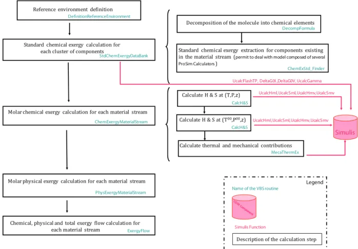
Fig. 7shows the flowchart of the exergy calculator dedicated to the calculation of physical and chemical exergy of a material stream. Three main procedures to calculate exergy of a material stream are explained as follows:

B Definition Reference Environment: This procedure is used to

define the conditions for the reference environment. The database of standard chemical exergy proposed by Rivero and Garfias[15] is used at the fixed temperature, pressure and composition.

B PhysExergy Material Stream: This procedure calculates the

physical exergy of the material stream. It uses procedure of CalcH&S to call enthalpy and entropy functions from Simulis thermodynamics.

B ChemExergy Material Stream: This procedure calculates the

chemical exergy of the material stream starting with calling StdChemExergy DataBank as a procedure to calculate the standard chemical exergy of the component found in the flowsheet based on the calculation methodology of Rivero and Garfias[15]. ElementStdChemEx as a database containing the chemical exergy of all elements including the standard database available with Simulis

thermodynamics with a subroutine of DecompFormula which break down each chemical compound into its constituent chemical elements, are matched together to calculate the chemical exergy.

3. Exergy balance and exergy analysis

Given the procedure dedicated to the calculation of exergy of individual streams, it is now possible to carry out exergy balance. Contrary to energy balance directly deduced from the first law of thermodynamics, exergy balance is deduced from the first and second laws of thermodynamics and requires a contribution of the engineer. Indeed, to enable the evaluation of internal and external losses thanks to exergy balances, first waste streams have to be distinguished from useful ones.

Fig. 5.Carnot cycle.

in in

s

h ,

h ,

_out

s

_out

Process Module Q Utility (Heat Source)

3.1. Waste stream vs. useful streams

The generic system illustrated in Fig. 8. can either represent a single unit operation, a global flowsheet or a part of a flowsheet. In this system, inputs material, heat and work are transformed into output ones by thermal and chemical operations. In such a system, some material and heat output streams are not useful ones and can be considered as waste streams (it can be waste materials that need to be recycled). Energy and exergy balances do not consider these waste streams in the same way.

As illustrated in Eq.(25), for energy balances deduced from the first law of thermodynamics, waste and useful streams do not need to be distinguished:

H_Minþ Qinþ Win ¼ HoutM þ Qoutþ Wout (25)

Likewise, to write exergy balance, total exergy input and total exergy output are given by the sum of input and output exergy associated with material, work and heat:

Bin ¼ X NSin M i ¼ 1 Bin_M;iþX NSin Q i ¼ 1 Bin_{Q ;i}þX NSin W i ¼ 1 Bin_W;i (26) Bout _¼ X NSout M i ¼ 1 Bout M;iþ X NSout Q i ¼ 1 Bout Q ;iþ X NSout W i ¼ 1 Bout W;i (27)

Fig. 7.Calculation of exergy of material streams in ProSimPlus

S

y

st

e

m

Waste Material Streams

Waste Heat out waste Q,

B

out waste M,

B

out waste

B

Product & By-Product Material Streams Heat Output out useful Q,

B

out useful M,

B

Work Output out useful W,

B

out useful

B

out

B

Inlet Material Streams Work Input in W

B

in M

B

Heat Input in Q

B

in

B

Contrary to energy balance, the strength of exergy balance relies on the capacity to estimate the exergetic efficiency of the process by classifying the output stream into “useful” or “waste” streams. As a consequence, the exergy of heat and material streams must be expressed as follows:

Bout

M ¼ BoutM;usefulþ BoutM;waste (28)

Bout

Q ¼ BoutQ ;usefulþ BoutQ;waste (29)

Furthermore, as all work output is assumed to be as “useful”, one can write:

Bout W;waste ¼ 0 (30) Bout_waste ¼ X NSout M;waste i ¼ 1 Bout_M;waste;i (31)

As a consequence, the total output exergy flow can be expressed as follows: Bout useful¼ X NSout M;useful i¼1 Bout M;useful;iþ X NSout Q;useful i¼1 Bout Q;useful;iþ X NSout W;useful i¼1 Bout W;i (32)

Using the “useful” and “waste” streams concept, the exergy balance can now be written. However, contrary to energy balance, another term corresponding to the exergy destroyed in the system (due to irreversibility of the process) must be introduced in the output terms. Then we have:

Bin _{¼ B}out

usefulþ BoutwasteþI (33)

where underlined term is “external exergy loss” and “I” represents the “internal exergy loss”. These two terms will be discussed in detail in the next section.

Finally, the resulting exergy balance can be written as follows:

X NSin M i¼1 Bin M;iþ X NSin Q i¼1 Bin Q;iþ X NSin W i¼1 Bin W;i¼ X NSout M;useful i¼1 Bout M;useful;iþ X NSout Q ;useful i¼1 Bout Q;useful;i þ X NSout W;useful i¼1 Bout_W;iþ X NSout M;waste i¼1 Bout_M;waste;iþ I ð34Þ The second law of thermodynamics complements and enhances the energy balance by enabling evaluation of both the thermody-namic value of an energy carrier, and the real thermodythermody-namic inefficiencies and losses of processes or systems[17].

3.2. Internal and external exergy loss 3.2.1. Internal exergy loss

Internal exergy losses, also called “irreversibility” or “exergy destruction” by Tsatsaronis [17], is deduced from the entropy generation and the environment temperature. According to the second law of thermodynamics, irreversibility is always positive.

In practice, for all real processes the exergy input always exceeds the exergy output, this unbalance is due to irreversibilities induced by the thermodynamic imperfection of process operations. The irreversibility phenomena fall in three types: non-homogeneities, dissipative processes and chemical reactions. Non-homogeneities are caused by mixing of two or more systems with different

temperature (T), pressure (P) or concentration (z). Regarding the dissipative effects, mechanical friction can be evoked. Finally, the entropy generated in chemical reactors is proportional to the advancement of the reaction and the affinity of the reaction itself defined using the stoichiometric coefficients and chemical poten-tials[19]. AlthoughTable 3is not exhaustive, it enumerates the major sources of irreversibility and gives us some clues taken from literature[2,7,20e23] for process improvement on each class of unit operation.Table 3can be extended to cover all the unit oper-ations especially using general commandments by Leites et al.[24]

for reducing energy consumption. 3.2.2. External exergy loss

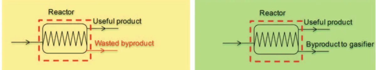
External exergy loss is associated with material streams rejected into the environment. For example, the flue gas emitted from a fired heater is still hot enough relative to the reference environment temperature (usually 25 C). By definition, the exergy associated with the flue gas is called external exergy loss of the fired heater.

To see how to reduce external exergy losses, let us take an example of a reactor represented inFig. 9. Depending on the use of the output byproduct of the reaction, external exergy losses will take different values. In the first case, output byproduct is simply emitted to envi-ronment. In this situation, output byproduct must be considered as a waste material and the absolute value of external exergy loss will be equal to the exergy associated with byproduct rejected to the envi-ronment. The exergy balance can be written as follows:

Bin_M ¼ Bout_M;usefulþ Bout_M;wasteþ I (35) and

Bout_M;useful ¼ Bproduct (36)

In the second case, on the contrary, the byproduct of the reaction can be valorized in a gasifier as a fuel. In that situation, the byproduct can be considered as a useful stream and the external exergy loss for the control surface inclosing the reactor will be zero:

Bout

M;waste ¼ 0 (37)

Here, the exergy balance becomes:

Bin_M ¼ Bout_M;usefulþ BoutM;wasteþ I (38) This simple example shows that exergy balance is highly dependent on the utilization of streams. Therefore, systematic calculation of such balances in process simulators such as ProSimPlus

requires a more precise definition of the role of the streams. There are different possible ways to exploit the exergy associated with the waste streams as addressed by Szargut et al.[7]. For example, if the temperature of the waste heat is high enough, waste heat recovery using heat exchanger networks can be an alternative. However, for the low-grade waste heat[25], heat pump

[26]or absorption refrigerator[27]can be installed to exploit its physical exergy. To reduce external exergy losses associated with chemical exergy, combustible waste can be used as a fuel for combustion. Utilization of the non-combustible waste as a secondary raw material is an alternative to recuperate wasted chemical exergy[7].

3.3. Exergy efficiency

To perform an effective exergy analysis, it seems essential to define indicators measuring the exergetic performance of a process

and identifying the unit operations that need to be improved. In the literature, several formulations have been proposed for the exergy efficiency. The simple efficiency[28]is simply the ratio between all exergy inputs and all exergy outputs.

h

_I ¼ B out

B_in ¼ 1 $

I

B_in (39)

Although it is easy to be calculated, the simple exergy efficiency does not provide a clear vision for the cases in which the significant amount of waste (i.e. external exergy loss) is produced.

To solve this problem, coefficient of exergy efficiency taking into account external losses[29]is defined:

h

_II ¼ B out_{$ B}out waste Bin ¼ BPRODUCT Bin ¼

h

I$ Bout waste Bin (40)

However, this new formulation for exergy efficiency gives a valid evaluation of the performance of a system only when all the components of the incoming exergy flow are transformed to other components of exergy. For example, a hydrocarbon stream heating up in a heat exchanger where only its physical exergy changes, has a high chemical exergy which does not affect at all. In other words, the role of the heater is to heat up the hydrocarbon stream (i.e. physical exergy change) not to change its chemical composition (i.e. chemical exergy change). Although this exergy efficiency gives a value close to unity for the case of this heater, it does not mean the heater is operating perfectly. Therefore, one might deduce the transiting exergy[29]as the unchanged part of exergy which does not participate in the process. This might be the main idea to develop the intrinsic exergy efficiency [29] which deduces the transiting exergy from both the exergy input and the exergy output. However, intrinsic exergy efficiency is not only complicated, but it also does not account for the external exergy losses. Utilizable exergy coefficient [30] might be regarded as the most rigorous exergy efficiency despite its complicated calculation procedure as it can measure the energy efficiency, the waste reduction and the efficient use of raw materials.

Besides these exergy efficiencies, rational efficiency[2]is a ratio of the desired exergy output to the used exergy. It is rigorous enough to evaluate the performance of the most commonly used unit operations if their objective are precisely defined and different components of exergy of material stream (e.g. chemical, thermal and mechanical) are known.

J

¼ Desired Exergetic Effect

Used Exergy ¼

D

B_{desired output}

D

B_used (41) where

D

Bdesired outputis determined by examining the function of the system and of course does not include external exergy loss. The

D

Bdesired outputrepresents the desired result produced in the system.

D

Busedrepresents the net resources which were spent to generate the product.

The major difficulty in this type of efficiency is the evaluation of

D

Busedand

D

BDesired Output. Contrary to the simple efficiency, it is necessary to define precisely the objective of the operation. This is not straightforward as it will be shown later. It is sometimes possible to define this objective in different ways for a single unit operation. The desired exergy output of the unit operation is defined by the user. After introducing Busedand Bdesired output, the exergy balance becomes:

D

B_used ¼

D

B_{desired output}þ I þ Boutwaste (42) Using Eq. (41)in connection with the Eq.(42), the following alternative form of the rational efficiency can also be obtained:

J

¼ 1 $I þ B

out waste

D

B_used (43)

Eq.(42)shows that if external exergy losses and desired exer-getic effect are known, the exergy balance will allow deducing the Bused. To illustrate this methodology, let us take the example of a two-stream heat exchanger shown inFig. 10.

Table 3

Internal exergy loss and its sources. Unit

operation

Sources of irreversibility Improvement ways

Reactor Low conversion Recycle the non-converted feed Exothermic reaction Raise the temperature Endothermic reaction Reduce the temperature Temperature difference

of cold feed and hot reaction medium

Pre-heating of feed

Concentration gradients Increase reaction stages as much as possible

Mixing of streams Mixing as uniform as possible Distillation

column

Concentration gradients Use intermediate reboiler Equal partition of driving force Improper separation

sequence

Optimize distillation sequencing Pressure drop and

mechanical friction

Optimize the hydraulic of the column

Bubble-liquid mass transfer on the tray[23]

Optimize the hydraulic of the column

Thermal gradients Introduce feed in a proper tray[20]

Splitting feed Heat

exchanger

Temperature difference Use as low as possible driving force

Non-uniform gradient Use an uniform gradient Pressure drop Reduction of number

of baffles

Low heat transfer Optimize the flow velocity[7]

Cold utility

Refrigeration Minimize use of sub-ambient system and replace it with cooling water[21]

Thermal difference Use as high level as possible Use of external utilities Maximize process steam

generation Throttling

valve

Pressure drop Replacement by a steam turbine (for temperature greater than the ambient) Steam

boiler

A chemical reaction for oxidation of the fuel[22]

Preheating of combustion air An internal heat transfer

between high temperature product and the unburned reactant[22]

Use as low driving force as possible

A physical mixing process[22]

Mix it as uniform as possible

A diffusion process where the fuel and oxygen molecules are drawn together[22]

Make it as gradually as possible

High heat capacity of combustion products

Oxygen enrichment[2]

Isobar combustion Isochoric combustion[2]

Compressor Hot inlet streams Temperature reduction of inlet streams or between the stages by intercooler Steam

turbine

Low temperature of steam

Use inter-heater (e.g. super-heater) between the stages Pump Hydraulic friction Optimize the hydraulic of

system

Mixer Temperature difference Isothermal mixing Pressure difference Isobar mixing Composition difference Mixing as close as

Basically the function of a heat exchanger is to change the thermal exergy of one stream at the expense of exergy change of the other stream. Let us assume the function of heat exchanger under consideration to be increase of thermal exergy of cold stream:

D

Bdesired output ¼ BDcold outT $ BDcold inT (44) Rewriting the exergy balance around the heat exchanger considering all component of exergy, we obtain:

BDT

cold inþ BDcold inP þ Bchcold in !

þ BDT

hot inþ BDhot inP þ Bchhot in !

¼ BD_{cold out}T þ BDcold outP þ Bchcold out !

þ BDT

hot outþ BDhot outP þ Bchhot out !

þ I þ Boutwaste (45)

Separating the term that is equal to function of the unit opera-tion, we have:

BD_{cold out}T $ BD_{cold in}T ¼ BD_{cold in}P $ BD_{cold out}P !þ Bch_{cold in}$ Bch_{cold out}!

þ BDT

hot inþ BDhot inP þ Bchhot in !

$ BDT

hot outþ BDhot outP þ Bchhot out !

$ I $ Bout_waste (46)

Canceling out the chemical exergy at the inlet and outlet and rearranging Eq.(45)based on the Eq.(46), Busedis the right side of the Eq.(47).

BDT

cold out$ BDcold inT !

þ I þ Boutwaste ¼ BDcold inP $ BDcold outP

!

þ BDT

hot inþ BDhot inP !

$ BD_{hot out}T þ BD_{hot out}P ! (47) Then applying Eq.(41), rational exergy efficiency will be given:

If pressure drop is negligible, we get the traditional form of exergy efficiency:

J

¼

D

Bdesired output

D

Bused ¼

BDT

cold out$ BDcold inT

BDT

hot in$ BDhot outT

(49) This example shows that for each unit operation, a function needs to first be defined to calculate the rational exergy efficiency. It means that it needs interaction of the user as always one unit operation does not have the same function. Rational efficiency needs to be defined precisely for all unit operations as listed in

Table 4. In addition, rational efficiency needs a drastic breakdown of different components of exergy of material stream as chemical, thermal and mechanical.

Having reviewed the different kinds of exergy efficiencies, it can be concluded that the rational exergy efficiency is not complicated as the “exergy efficiency with transiting exergy” and is rigorous enough unlike “simple exergy efficiency”. Therefore, the rational exergy efficiency has been chosen to be implemented in ProSimPlus

for an adequate exergy analysis.

3.4. ProSimPlus

implementation

As pointed out in the previous section, rational exergy efficiency needs a clear function per each unit operation. In addition, the Fig. 9.External exergy loss for a reactor.

HOT IN HOT OUT

COLD IN COLD OUT

Fig. 10.Two-stream heat exchanger.

J

¼

D

Bdesired output

D

Bused ¼

BDT

cold out$ BDcold inT

BDP cold in$ B DP cold out ! þ BDT hot inþ B DP hot in ! $ BDT hot outþ B DP hot out ! (48)

T able 4 Rational ef fi ciency for the most commonly used unit oper ations.

–

waste streams should be specified. Having known the function of the unit operation and waste streams, the

D

Busedcan be calculated based on the exergy balance around the given unit operation. Therefore, to implement rational exergy efficiency a semi-automated way has to be followed as shown inFig. 11. As a first step a zone is defined by the user. Then, the simulator automatically provides us with a table (see Table 5) as well as exergy of all streams. Next, the role of each stream (waste vs. useful) is defined by the user in the table given by ProSimPlus

. However, ProSimPlus

can consider all the output streams as waste streams by default. Then the user can change it to the useful. Finally, the process simulator can provide the necessary criteria for analysis such as rational exergy efficiency. To facilitate calculation of the rational exergy efficiency, the desired exergy effect can be auto-mated and embedded in ProSimPlus

for the most commonly used unit operations. In addition, for units which do not have always the same function, a set of possible efficiencies can be proposed by ProSimPlus

which will be finally chosen by the user. 4. Case study

To show the applicability of exergy analysis for energy optimi-zation of a chemical or thermal process in ProSimPlus

, a simple process found in the literature[4]has been enriched and analyzed.

4.1. Process description

Fig. 12represents ProSimPlus

flowsheet for a stabilization train of natural gas containing traces of oil[4]. To satisfy the specification of marketing, natural gas needs to be stabilized. In this process, the natural gas (C1 to C8 hydrocarbons) is separated into a stabilized condensate (C4 to C8 hydrocarbons) and a saleable gas (C1 to C4 hydrocarbons). As the amount of natural gas in our case is not so high, a full Natural Gas Liquid (NGL) recovery train is not economically justifiable and the simple stabilization scheme shown in the right section ofFig. 12is chosen[4].

Along of this process, a rich gas is heated in three heaters followed by separators (F101, F102 and F103) where the inlet gas streams are flashed. At each step, the outlet liquid stream is sent to the next flash where the pressure is reduced further. The liquid stream from the last flash is the stabilized condensate. On the other hand, the outlet gas streams from all of the separators (F101, F102 and F103) are mixed together with same pressure to obtain a stabilized gas product stream with the desired specifi-cations[4].

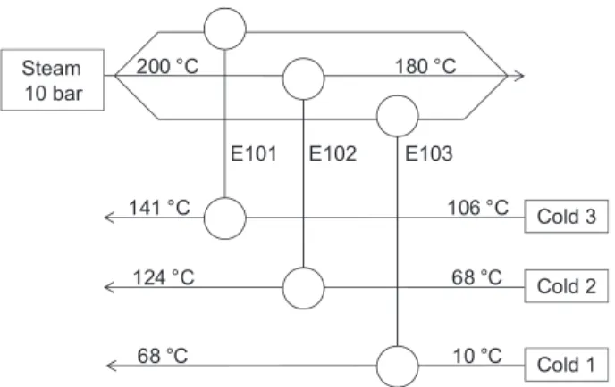
To meet heating requirement of the process, a relative high pressure (HP) steam at 10 bar with 80 C degree of superheat for all three separation stages is used as shown inFig. 13. The process streams are heated up by the steam condensation in heat exchangers and condensate is throttled down to 3 bar. The condensate is returned at 3 bar and is mixed with the boiler water makeup to feed the steam boiler. Note that a small portion of steam at 10 bar is used in the deaerator to separate air from return-condensate. As well as steam heating, electricity is required to drive the compressors (C101 and C102) at the second and third stages of stabilization where pressure drop causes the flash sepa-ration. The required electricity for the base case is imported from the external electricity grid.

4.2. Simulation

All the required data and specifications for the simulation of the process and the utility system are given inTables 6e8. As reported inTable 7, the outlet temperature of heater E101, E102 and E103 has to be fixed at 68, 124 and 134 C. Therefore, splitting ratio of the splitter distributing the steam among the three heaters, and water make-up flowrate will be varied to obtain a converged simulation. In addition, to keep the flue gas temper-ature equal to 200 C (higher than the acid dew point), the fuel flowrate will be varied.

To calculate the thermodynamic properties, two different ther-modynamic models are defined:

B The PengeRobinson equation of state: for the NGL process

and the fuel combustion sections.

B The water specific thermodynamic model: for simulation of

the utility system.

Note that in this case study, heat losses to the environment has been neglected.

4.3. Exergy analysis

By offering the possibility to make automatic calculation of exergy of material and heat streams and to present the result of exergy balance in different forms such as pie or bar diagram for the given process or utility zone in an automated way, ProSimPlus simulator facilitates exergy analysis on the process[31].

As demonstrated earlier, the exergy analysis requires the defi-nition of the utilization of streams (i.e. waste or useful) by the user. In this case study, all the material streams leaving the process are useful whereas all the material output streams in the utilities system are considered as waste streams as they are directly rejected

into the environment. As a consequence, in this specific case study, external exergy loss will only be associated with the utility system. 4.3.1. Internal/external losses

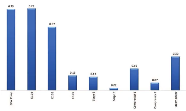
By representing the external and internal exergy losses occur-ring in each of the unit operations are on a bar diagram (seeFig. 14), one can identify technical solutions to improve the performances of the process. While the internal exergy losses (or irreversibilities) can be reduced through development of the process or technology improvement, reduction of external exergy losses requires a thermal, mechanical and chemical treatment of effluents.

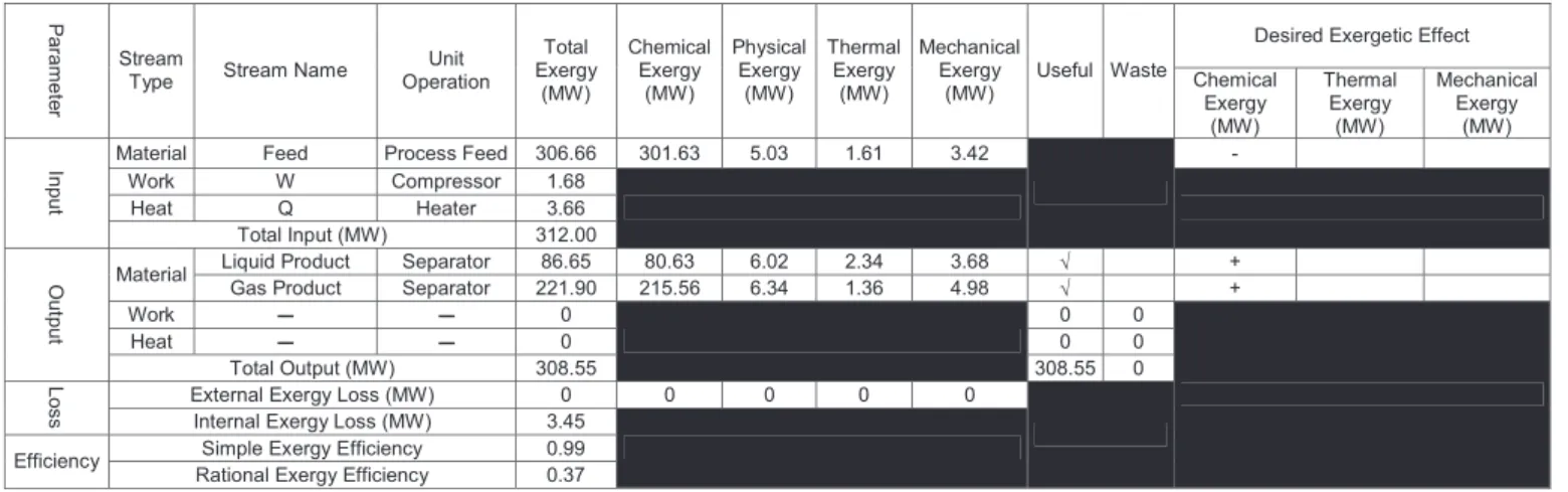
As can be seen inFig. 14, the largest irreversibilities occur in the steam boiler. Intrinsic irreversibility due to the combustion is unavoidable; however, according to Table 3 solutions exist to reduce the internal exergy loss such as prehearing of combustion air though an economizer. The second-largest irreversibility occurs in the heat exchanger network because of the large temperature difference between hot and cold streams. As listed inTable 3, to reduce exergy losses, as low as possible driving force between the hot (steam) and cold (process) streams have to be used. In addition, Table 5

A typical table given by the exergy assistant in ProSimPlus

to distinguish waste vs. useful streams.

Desired Exergetic Effect

P a ra m e te r Stream

Type Stream Name

Unit Operation Total Exergy (MW) Chemical Exergy (MW) Physical Exergy (MW) Thermal Exergy (MW) Mechanical Exergy (MW)

Useful Waste _Chemical Exergy (MW) Thermal Exergy (MW) Mechanical Exergy (MW)

Material Feed Process Feed 306.66 301.63 5.03 1.61 3.42

-Work W Compressor 1.68 Heat Q Heater 3.66 In p u t Total Input (MW) 312.00

Liquid Product Separator 86.65 80.63 6.02 2.34 3.68 √ + Material

Gas Product Separator 221.90 215.56 6.34 1.36 4.98 √ +

Work 0 0 0 Heat 0 0 0 O u tp u t Total Output (MW) 308.55 308.55 0

External Exergy Loss (MW) 0 0 0 0 0

L

o

s

s _{Internal Exergy Loss (MW) 3.45}

Simple Exergy Efficiency 0.99 Efficiency

Rational Exergy Efficiency 0.37

Steam 10 bar 260 °C Return Condensate 3 bar, 134 °C Deaerator Boiler E101 E102 E103 Condensate Purge Water Make-up Water Loss Vent Flue Gas Cold 1 Hot 1 Cold 2 Hot 2 Cold 3 Hot 3 BFW Pump F101 F102 F103 68 °C 124 °C 141 °C Gas Product NGL Process Feed 10 °C, 4125 kPa, 490 kmol/hr Legends Utility Process C102 C101 Fuel Air

throttling valves cause relatively high irreversibilities that could have been easily avoided by their replacement with steam turbines as reported inTable 3.

The external exergy losses associated with the steam boiler is due to its flue gas. To reduce this external loss chemical recu-peration of flue gas [32]can be applied. To exploit the thermal component of exergy of hot streams such as the vent of dearetor and condensate purge, a waste heat exchanger might be a solution.

Exergy analysis of this flowsheet has so far identified and quantified the available thermal energy in a process that could have been potentially exploited to meet energy demands elsewhere on the process or even on the industrial site. At this point, however, exergy analysis cannot deal with the energy integration of the process. Coupling of exergy analysis with a pinch analysis [33]

could be helpful to provide solutions relevant to the reduction of exergy losses in the process.

4.3.2. Exergy efficiency

Figs.15and16represent the simple and the rational exergetic efficiencies of each unit operation. Whereas simple exergy effi-ciencies are very easy to calculate (see Eq.(39)), a desired exergetic effect has to be defined for calculation of rational exergy efficiency. For example, the major desired exergetic effect for the three heaters is to heat up the process streams. Concerning the NGL process as a whole, its desired effect relies on the chemical exergy change between input and output. The part of chemical exergy which remains unchanged between the input and the outputs of the process is not included in the rational exergetic efficiency calcula-tion. As shown in Fig. 15, the simple exergy efficiency is quite restrictive for this case where the major part of exergy input consists in the chemical exergy which remains unchanged. As can be seen from comparison between Figs.15and16, rational exergy efficiency is much more informative.Fig. 15shows that most units

operations are operating with efficiency close to unity, but rational exergy efficiency inFig. 16gives a real thermodynamic picture by presenting the imperfection occurring in the unit operations. The units which suffer from thermodynamic imperfection can be identified and improved to obtain a better performance. For example, comparing the heater E101, E102 and E103, the lowest rational exergy efficiency belongs to heater E101 where a relative high pressure steam is used to heat up the process stream of the first stage. Working with a low pressure steam can significantly reduce irreversibility by reduction of minimum approach temperature.

The advantage of analysis of exergy efficiencies rather than the exergy losses relies on the possibility to quantify the potential for improvement of each unit operations[34]: the lower exergy effi-ciency, the higher will be the potential for improvement. For example, although BFW pump has the same exergy efficiency as E103, its small exergy losses do not justify its revamping for exergy loss reduction. On the other hand, E101 has lower exergy efficiency, but it has higher exergy losses which means its small potential for improvement can finally reduce significantly the total exergy losses.

Comparing the absolute exergy losses with exergy efficiency, the order of unit operations is different. In addition, two unit opera-tions with the close exergy efficiency can have different exergy losses. For example, exergy efficiency of BFW Pump is the same of E103, but it has 0.5 kW exergy losses which is very small compared to E103 with 36.6 kW exergy losses. This is mainly due to the properties of flow coming into and out of the given unit operation such as temperature, pressure, composition and flowrate. As boiler feed water in the liquid state does not carry high quantity of exergy, 73% exergy efficiency cannot cause significant exergy losses. On other hand, exergy input of E103 is very high as the high exergetic steam (relative high pressure and temperature) are entering into the E103. Therefore, 73% exergy efficiency for E103 causes 36.6 kW exergy losses. E103 E102 E101 180 °C 200 °C Steam 10 bar 68 °C 10 °C _{Cold 1} 124 °C 68 °C _{Cold 2} 141 °C 106 °C _{Cold 3}

Fig. 13. Grid diagram of heat exchanger network for the base case.

Table 6

Specifications and variables of action for the base case.

Specification Variable of action

Outlet temperature of heater E101 ¼ 68 C

Splitting ratio of the splitter 1 and 2 Outlet temperature of heater

E102 ¼ 124 C

Splitting ratio of the splitter 1 and 2 Outlet temperature of heater

E103 ¼ 134 C

Water makeup flowrate Flue gas temperature ¼ 200 C Fuel flowrate

Table 7

Composition of feed.

Compound Mole fraction

Methane 0.316 Ethane 0.158 Propane 0.105 i -Butane 0.105 n-Butane 0.105 i -Pentane 0.053 n-Pentane 0.053 n-Hexane 0.027 n-Heptane 0.026 n-Octane 0.026 n-Nonane 0.026 Table 8

Input data for simulation of process.

Feed conditions 10 C and 4125 kPa

Outlet temperature of Heater E101 68 Outlet temperature of Heater E102 124 Outlet temperature of Heater E103 134

Feed flowrate 490 kmol/h

Stage 1 pressure drop 0 kPa

Stage 2 pressure drop 2075 kPa

Stage 3 pressure drop 1700 kPa

Gas Product pressure 4125 kPa

C101 adiabatic efficiency 75%

4.3.3. Proposal of a retrofit scheme

Having pinpointed the sources of exergy losses, the next step consists in determining a retrofit scheme based on the analysis of sources of irreversibilities. Although external exergy losses contribute in total exergy losses as well as internal exergy losses, reduction of internal exergy losses which originate from the heart of thermal and chemical process can consequently reduce external exergy losses. In other word, if the internal exergy losses are reduced, consequently the external exergy losses will be reduced as well.

The analysis ofFig. 16permits to identify the less efficient unit operations that need to be improved:

( Steam boiler: Prehearing of combustion air though an econo-mizer as pointed out earlier.

( Compressor: Although the temperature reduction of inlet stream can reduce exergy looses (seeTable 3), there is a risk of condensation of natural gas liquid in the compressor.

Therefore, the temperature of inlet stream has to be kept as it is in the base case.

( Heat exchanger: To reduce its irreversibilities, it is necessary to reduce the driving force between hot and cold stream. For obvious reasons, the process streams cannot be modified; thus, it is decided to reduce the inlet temperatures of the steam by its expansion. For that purpose, steam turbines are preferred over the simple expanding valves as the steam turbines can provide the required shaft power for stages 2 and 3. To keep the steam hot enough to meet the heating demand of the process, the steam is expanded to 4.5 bar for the last stage and 3 bar for the first and second stages. Note that compared to the base case, the degree of superheat of steam generated by the boiler, is fixed to be 80 C to avoid the steam condensation in the steam turbine which can damage the machine.

The improved configuration of the process and its grid diagram are presented in Figs.17and18. To simulate the modified flowsheet, Fig. 14.Internal and external exergy losses (kW) for the base case.

as reported inTable 7, the outlet temperature of process streams in heater E101, E102 and E103 has to be fixed to 68, 124 and 134 C. Therefore, splitting ratio of the splitter 1 and 2 distributing the steam among the heaters, and water make-up flowrate will be modified by the simulator. In addition to keep the flue gas temperature equal to 200 C (higher than the acid dew point), the fuel flowrate will be modified as listed inTable 6.

Table 10 shows that use of low-pressure steam for heating reduces both fuel and water demand while increases cogeneration potential as more latent heat can be taken from the condensation of steam in the lower pressure. As listed in Table 9, performance improvement of the integrated process is noticeable based on several criteria which makes analysis of the process very complex. To fill this gap and facilitate further optimization of the process, the rational exergy efficiency proposes an aggregated criterion including all the aspects listed in theTable 9. As the process cannot undergo any modification, therefore it is left out of the optimiza-tion. The exergy efficiency will be defined only for the utility system where the ‘desired effect’ of the utility can be defined as heating of the three process streams (Cold 1, Cold 2 and Cold 3) and produc-tion of shaft power required for compression of the streams coming out of stages 2 and 3:

where the underlined terms in the nominator represent the process, and the rest is standing for the utility system. The desired exergetic effect is taken to generate shaft power and heat up the process streams at the expenses of exergy supplied by the differ-ence between input material (i.e. fuel of steam boiler, water make-up, required shaft power of pump) and effluents (i.e. flue gas, vent, water loss and condensate purge). As noted earlier, this term

includes the excess shaft power available for the electricity grid, the consumption of all natural resources (e.g. fuel, water) and the wastes rejected to the environment (e.g. flue gas, steam vent) in a single criterion which is useful for analysis of performance of the system as a whole.

4.4. Estimation of the capital cost of the retrofit schemes

Reducing the provided stream pressure necessarily results in a reduction of the minimum temperature approach and of course an increasing of the required surface area of heat exchangers E101, E102 and E103. To complete the analysis of the process, estimation the capital cost (CAPEX) of heat exchanger network (HEN) as a function of surface area needs to be performed. For that study, the costing law proposed by Hall et al.[35]has been adapted:

CostðUSDÞ ¼ 30800 þ 750A0:81 (51)

where A represents total heat transfer area. To use this costing law it is assumed that plant life is 6 years and capital interest is 10% per year. The heat exchangers are assumed to be made of carbon steel and operate under 10 bar in both sides of shell and tube.

Note that use of ProSimPlus

simulator permits to implement very easily the cost calculation. The use of another law more rele-vant for the considered case study would not be difficult to be implemented.

Using Eq.(51), investment cost of economizer will be 32 822.32 USD. Taking into account a profit from fuel saving, the installation of economizer results in 22% return on investment.

Fig. 16.Rational exergy efficiency for unit operations.

J

¼ BDT Cold 1$ BDHot 1T ! þ BDT Cold 2$ BDHot 2T ! þ BDT Cold 3$ BDHot 3T ! þWTurbine B_Fuelþ BWater Make$upþ WPump$ BFlue Gasþ BVentþ BWater Lossþ BCondensate Purge

4.5. Sensitivity analysis for exergetic optimization of the process As shown earlier, to reduce the exergy losses occurring in the steam distribution system, throttling valves have been replaced by steam turbines. The exhaust pressure of steam turbine have been fixed arbitrary to 4.5 and 3 bar to keep the steam hot enough to meet the heating demand of the process. The choice of steam levels in the design of utility systems is critical to ensure cost-effective generation of heat and power, and its distribution to the process. In a new design, pressures of steam levels can be readily optimized.

The results of a sensitivity analysis of the rational exergy effi-ciency and capital cost with the exhaust pressures of steam turbines are presented in Figs.19 and20. When fixing medium pressure (MP) steam level, the decrease of low pressure (LP) steam level results in an increase of the rational exergy efficiency: indeed in these conditions, the shaft power increases and the fuel demand decreases. The lower pressure of LP steam level, the higher is the potential for steam to be expanded in the turbine for power generation. In addition, the lower pressure the higher will be the latent heat taken from condensation of steam, consequently less

fuel is required to be fed to the steam boiler. As shown inFig. 19the rational exergy efficiency has the same trend when pressure of MP steam changes under the fixed conditions of LP steam main. Furthermore, as a consequence of pressure reduction, temperature of steam is reduced which leads to less minimum temperature approach in heat exchangers. Consequently, more area is required to exchange the fixed amount of heat which finally leads to higher capital cost of the heat exchangers.

As shown in Figs.19and20, both HEN cost and rational exergy efficiency are more sensitive to the pressure of LP steam level compared to the MP steam level due to use of LP steam in two out of the three stages. Therefore, minimum and maximum limit for LP steam main as a variable of optimization should be chosen with more precaution.

Note that this sensitivity analysis serves as a necessary step to create the required data for construction of Pareto frontier curve which will be used in an exergetic optimization described in the following section.

4.6. Bi-criteria optimization

In addition to the sensitivity analysis and due to the difficult interpretation of some results in rational exergy efficiency (Fig. 19) in terms of steam levels, a bi-criteria optimization task has been performed by ProSimPlus

to offer a decision support in retrofitting steps. However, it should be kept in mind that for retrofitting of existing systems, opportunities to change the steam level condi-tions are limited. The mechanical limitation for the steam mains limits a significant increase in steam pressure. Indeed, long term investment with a proper optimization of the steam levels may be economically viable, in spite of the fact that the short term investment cannot be justified[21].

E103 E102 E101 134 °C 154 °C LP Steam 3 bar 68 °C 10 °C _{Cold 1} 124 °C 68 °C _{Cold 2} 141 °C 106 °C _{Cold 3} 148 °C 188 °C MP Steam 4.5 bar

Fig. 18.Grid diagram of heat exchanger network for the retrofit scheme.

Table 9

Input data for simulation of utility.

Stack temperature 200 C

Degree of superheat of HP steam 80 C

Temperature of return condensate 134 C

Pressure of return condensate 3 bar

For revamped case: steam turbine isentropic efficiency (stage 1 and 2)

75% Fig. 17.Improved process & utility flowsheet.

4.6.1. Optimization framework

In this study, optimization tool of ProSimPlus

is used to perform a bicriteria (exergetic efficiency/investment cost) optimi-zation. The details of the optimization model are as follows: 4.6.1.1. Objective function. The purpose is to maximize the exer-getic efficiency calculated by Eq.(50)and minimize the HEN cost calculated by Eq.(51). It should be noted that minimizing the HEN cost does not correspond to minimum overall cost of utility systems. However, it is extremely difficult to generalize the capital investment to be required in the conceptual stage of process design, and the current study focuses on the maximizing exergy efficiency for the utility systems, which provides sufficient information and reliable guidance for achieving an effective design in the later stage of detailed design. Two steam mains (MP and LP) are used in the current optimization model based on the needs and operating characteristics on the plant. An ε-constraint procedure is carried out and a Pareto frontier curve[36]is constructed for support of decisions making.

4.6.1.2. Model constraints. In order to maintain feasibility of heat recovery across steam mains, a set of constraints is needed.

Temperature of all hot streams (steam) should be always greater than temperature of all cold streams (process) as follows:

T_{LP SteamðinÞ}$ THot 1) 10 (52) T_{LP SteamðinÞ}$ THot 2) 10 (53) T_{MP SteamðinÞ}$ THot 3) 10 (54) TLP SteamðoutÞ$ Tcold 1) 10 (55) TLP SteamðoutÞ$ Tcold 2) 10 (56) T_{MP SteamðoutÞ}$ Tcold 3) 10 (57)

Obviously, the exhaust pressure of second stage of turbine should be lower than the first stage:

PMP SteamðinÞ$ PLP SteamðinÞ>0 (58)

4.6.1.3. Equality constraints. The utility system has only one equality constraint which is to fix the flue gas temperature to a temperature higher than the acid dew point (473 K).

Table 10

Comparison of performance of the base case and integrated retrofit configurations. Fuel demand

(kg/hr)

Water makeup (t/hr)

Degree of superheat of steam from boiler

Electricity requirement Internal exergy losses (MW) External exergy losses (MW) Base case 224.6 1.03 20 C 191 (kW) 3.007 0.292 Retrofit 220.1 0.63 80 C 0 2.628 0.170 0.12 0.13 0.14 0.15 0.16 0.17 0.18 2 3 4 5 6 7 8 9

Rational Exergy Efficiency

LP Pressure (bar) MPPressure = 8 bar MPPressure = 7.5 bar MPPressure = 7 bar MPPressure = 6.5 bar MPPressure = 6 bar MPPressure = 5.5 bar MPPressure = 5 bar MPPressure = 4.5 bar

120000 121000 122000 123000 124000 125000 126000 127000 128000 129000 130000 131000 132000 133000 134000 135000 136000 137000 138000 139000 2 3 4 5 6 7 8 9

HEN Cost (USD)

LP Pressure (bar) MPPressure = 8 bar MPPressure = 7.5 bar MPPressure = 7 bar MPPressure = 6.5 bar MPPressure = 6 bar MPPressure = 5.5 bar MPPressure = 5 bar MPPressure = 4.5 bar

Fig. 20.HEN cost (USD).

0.12 0.13 0.14 0.15 0.16 0.17 0.18 120000 122000 124000 126000 128000 130000 132000 134000 136000 138000

Rational Exergy Efficiency

HEN CAPEX (USD) MP=6.5bar, LP=4.9 bar