The Effects of Penalty Information on Tax Compliance: Evidence from a New Zealand Field Experiment
by
Norman Gemmell† and Marisa Ratto‡
January 2017
ABSTRACT
The ‘standard’ Allingham-Sandmo-Yitzhaki (ASY) model of tax evasion predicts effects on compliance which depend on the perceived probability of detection, tax rate and penalty for evasion. Compliance effects of detection probabilities and tax rates have been extensively tested empirically, but penalty effects are rarely tested explicitly. This paper examines the effects of late payment penalties on tax compliance based on an experiment involving thousands of New Zealand goods and service tax (GST) payers. Firstly, we adapt the ASY model to allow for less than full enforcement of discovered evasion, and apply this to the late tax payment context. Secondly, based on a field experiment involving a specific compliance intervention, we examine how taxpayers respond when given different penalty information. We also consider differences between taxpayers’ stated intentions to comply during the experiment and subsequently observed compliance. Results suggest that differences in penalty information given to taxpayers, and reductions in penalty rates both affect taxpayers stated intentions to comply (pay overdue tax and penalties) as predicted. However, subsequently observed responses generally appear unresponsive to penalties. Nevertheless, various individual taxpayer characteristics are identifiable that affect both compliance intentions and actual behaviour.
JEL codes: H26, C93
Keywords: tax evasion, late payment penalties, tax experiment, goods and service tax
† Victoria University of Wellington, Wellington, New Zealand
‡ Corresponding author : Université Paris-Dauphine, Place du Maréchal de Lattre de Tassigny
1. Introduction
The so-called ‘standard model’ of tax evasion due to Allingham and Sandmo (1972) and Yitzhaki (1974) – hereafter labelled the ‘ASY model’ – has been subjected to widespread challenge and empirical testing – the former mainly with respect to its apparently counter-intuitive prediction that evasion is expected to be decreasing in the tax rate. Less controversially, the ASY model also predicts that compliance increases in the penalty rate applied to evaded tax. However, as Slemrod (2007, p.38) noted: “there has been no compelling empirical evidence addressing how noncompliance is affected by the penalty for detected evasion, as distinct from the probability that a given act of noncompliance will be subject to punishment”. Specific under-researched aspects include: whether high penalties elicit greater compliance as the ASY model predicts; how well taxpayers understand the penalty regime they face, and whether providing more accurate penalty information necessarily improves compliance?1
This paper explores these questions using the specific example of New Zealand’s Goods & Service Tax (GST) penalties,2 based on evidence from a field experiment involving several
thousand New Zealand GST payers in debt to the revenue authority. This was designed to test for the effect on GST debt repayment choices of differing levels of, and taxpayer information on, GST late payment penalties. The experiment involved offering a random sample of tax debtors a penalty discount if they agreed to enter a repayment arrangement, after first providing those taxpayers with penalty regime information in differing degrees of detail.
A particular advantage of the test in this context is that the ‘evaded’ outstanding tax is known to both the taxpayer and the revenue authority – New Zealand’s Inland Revenue department (IRD). The probability of detection in this case can therefore reasonably be treated as unity. That is, the experiment can be expected to reveal pure penalty effects uncontaminated by ‘probability of detection’ effects, allowing us to consider the degree of support for this aspect of the ASY model.
The remainder of the paper is organised as follows. Section 2 describes the New Zealand GST penalty regime and the compliance experiment undertaken by Inland Revenue. Section 3 then considers how the ASY model may be adapted to capture this particular form of non-compliance and penalty regime. Section 4 describes our empirical framework and the experiment data. Section 5 discusses the results for the experiment, and section 6 concludes.
2. The New Zealand (NZ) Penalty Regime and Experiment
As in many OECD countries, the Goods & Service Tax (GST) – NZ’s form of value added tax – is an important part of the overall tax system. It is also responsible for a large fraction of late tax payments in New Zealand. For example, IRD data show that in July 2015 total unpaid GST liabilities were around $1.5 billion, representing around 25% of all unpaid tax, second only to personal income tax debt at around 44% of the total. GST debt was owed by 81,689 GST
1 See Slemrod et al. (1995) and Skov (2016) for some evidence on penalties and the timing of tax payments for the
US and Denmark respectively. 2
GST is New Zealand’s version of a value added tax. Unusually among OECD VAT regimes it applies to almost all value added at a uniform rate (currently 15%), excluding financial services (exempt) but including all government value added activities.
payers in July 2015: 13.2% of total registered GST payers. However, almost half (46.5%) of all registered GST payers had been in GST debt at some point either currently or in the past.
IRD also groups the length of time GST payments have been overdue into three categories: <60 days, 60-90 days and >90 days, with the latter acknowledged as especially difficult to collect. Of the 13.2% of taxpayers in debt in 2015, over two-thirds (9.3%) had been in debt for longer than 90 days, representing almost 95% of the $1.5bn. total outstanding GST liability. In short, unpaid GST affects a large fraction of registered taxpayers and represents a large amount of outstanding tax liability, collection of which is a substantial non-compliance and enforcement resource issue.
2.1 The Penalty Regime
In common with a number of countries, the two main types of penalties levied on NZ taxpayers are a late filing penalty and late payment penalties. The late filing penalty is fixed as a dollar amount, from $50 to $500, differing by the type of tax (e.g. income tax, GST, etc.) and by some taxpayer characteristics (e.g. net income, accounting basis).
Late payment penalties have two components.
(i) An initial penalty in two stages: a 1% late payment penalty charged on the day after the due date and a further 4% penalty charged on amounts of tax and penalties unpaid seven days after the due date. Since the taxpayers considered here all have overdue tax of 60 days or more, below we simplify this penalty as a single 5% initial penalty, ignoring the 1/7 day distinction.
(ii) An incremental penalty charged at 1% per month for outstanding debt including initial penalties. This is equivalent to approximately 12.7% per year.
In addition, use-of-money interest (UOMI) is charged on all outstanding debt inclusive of penalties, with the rate varying according to market conditions. Since May 2016, this is 8.3% per year, reduced from a high of 14.2% in March 2007.3
When an individual owing penalties is unwilling or unable to pay outstanding debt to IRD immediately, the tax authority may offer an instalment arrangement to the taxpayer, or agree to one proposed by the taxpayer. This agreement triggers the cessation only of the incremental penalty, remaining in place as long as the taxpayer adheres to the instalment agreement. The initial 5% penalty remains payable, and UOMI continues to apply to all outstanding tax including penalties.
Letting
φ
be the initial 5% penalty and f represent the incremental penalty, the effective fine rate for the first $ of debt (the ‘extensive margin’) is given by (1 +φ
+ f)(1 + r) = 1.276 or 27.6%, while the ‘intensive’ marginal penalty rate applicable to each additional $ of debt is (1 + f)(1 + r) = 1.226 or 22.6%. Since f = 0 when in an instalment arrangement, this reduces the effective
3 Since 1997, the rate peaked at 14.7% in 1998. These are ‘debit rates’, linked to short-term market borrowing rates,
charged on outstanding debt to IRD. A much lower ‘credit rate’ (currently 1.6%) is paid on overpayments to IRD, linked to market-based short-term deposit rates.
‘extensive’ and ‘intensive’ penalties to 13.8% and 8.8% respectively.4 The percentage effective
penalty rates are therefore more than halved in an instalment arrangement.
The analysis below ignores late filing penalties, and concentrates on late payment penalties which were the focus of the experiment.
2.2 The Field Experiment
This experiment was undertaken by IRD from August 2014 to September 2014 and was part of a compliance ‘campaign’ or ‘intervention’ to encourage taxpayers with GST debt outstanding for between 60 and 90 days to repay their debts.5 From a total of over 4,400 debtors in the
campaign, a sample was randomly selected to enter the experiment, split into three treatment groups each of 333 or 334 taxpayers. The campaign sought to communicate with debtors by various means but those selected for treatment in the experiment were all targeted to receive a specific phone call to encourage them to pay their debts using one of three possible ‘scripts’ to open the conversation. All debtors had previously received at least one IRD letter seeking payment and mentioning penalties. The phone call (a standard IRD compliance tool) first requested immediate payment of the outstanding debt – a requirement of IRD’s code of practice. In the absence of an initial positive response, taxpayers in the treatment groups were offered a reduced-penalty instalment arrangement in which debt is repaid over a negotiated period, usually up to 2 years.
Specifically, the phone call differed between the three groups in terms of the information about debt-related penalties that was given to the taxpayer before offering the instalment option. In addition to the benefits of the delayed payment schedule via lower interest payments, the instalment option ‘turns off’ the incremental penalty, at 1% per month, that otherwise accumulates on outstanding debt.
3. Modelling Taxpayer Choices
In our context the non-compliance decision does not consist of under-declaring true income, as in the ASY model, but relates to late payment of the assessed due tax. Both the taxpayer and the tax authority are aware of the tax debt outstanding, even if the value of that debt may not be agreed. Though this ‘evasion’ has already been detected, where the taxpayer perceives a probability of permanently avoiding all or part of the debt (e.g. via a write-off), this may be treated as analogous to the ASY model’s perceived probability of detection. Rather than failing to detect the full tax liability, the tax authority in this case fails to enforce it. We define this more formally below as a perceived ‘probability of enforcement’,
π
.Before setting out the late tax payment model it is useful to summarise the key ASY model results (sub-section 3.1) before adapting those to the late payment context in 3.2.
4
The effective marginal penalty rate in instalments exceeds the interest rate since interest continues to apply to the fixed penalty; i.e. (1 + r + rφ).
5 IRD regularly undertakes compliance ‘campaigns’ as a tool to improve compliance for various taxes or tax credits.
These campaigns target specific segments of the non-compliant taxpayer population with strategies involving, for example, targeted phone calls, specially designed letters, and offers to negotiate over repayment periods, etc.
3.1 Allingham-Sandmo-Yitzhaki Model Results
The ASY model, as summarised by Sandmo (2005), takes gross income, W, as given, and considers the decision to evade some income, E, from tax, for a given tax rate, t, applied to declared income and a ‘penalty tax rate’, F > t, applied to evaded income if detected. With declared income equal to W – E, the taxpayer’s objective is to maximise utility, V, from income in two possible states – where evasion is undetected (hence net income, Y = (1 – t)W + tE) and where evasion is detected (hence net income, Z = (1 – t)W –( F – t)E.)
AS (1972) and Yitzhaki (1974) show that for a risk-averse taxpayer, and where penalties are levied as a fraction of evaded tax, tE, rather than evaded income, then some tax evasion is optimal if:
pF < 1 (1)
where F > 1 is the ‘penalty rate’ and FtE is the evaded tax inclusive of penalties; see Sandmo (2005, p.647). 6 Hence, the taxpayer prefers to evade some tax if the ‘expected penalty rate’, pF, is less than 1. It is this result that has generated extensive debate over the ‘puzzle’ that, for plausible values of p and F, it should be optimal for the vast majority of taxpayers to evade.7
The inequality in (1) may alternatively be expressed as:
p < 1/F (2)
that is, the probability of detection is less than the inverse of the penalty rate. Following Sandmo (2005), the right–hand side of (2) can be interpreted as a relative price of income in the states of detection and non–detection. The numerator of (2) is simply the ‘price’ of undetected evasion - each dollar of evaded tax is worth one dollar to the taxpayer, while the denominator is the price of a dollar of detected evasion, namely the penalty rate F > 1, giving a relative price of 1/F.
3.2 Applying the ASY Model to Late Tax Payments
Once their tax liability has been assessed, taxpayers have the choice of paying immediately, at time t, without penalty or delaying and incur penalties on the outstanding debt, at time t+1. Gemmell (2016) sets out a simplified two-period model of an individual taxpayer’s payment choice to clarify the incentives that may drive these taxpayer’s choices. We build on that analysis and consider a taxpayer who is already in debt (has already decided not to pay immediately) and is offered an instalment option, as this is the context of our experiment.
6
As in Sandmo (2005), the ‘penalty rate’ is defined here to include both the evaded tax and the added penalties applied; hence F > 1. The original AS paper, and some subsequent literature, use the term ‘penalty tax rate’ which is applied to evaded income, given here by tF; see Sandmo (2005, pp.646-7), Gahramanov (2009) and Gemmell (2016) for exposition.
7
For example if the perceived probability of detection is 0.10 (an order of magnitude suggested by various empirical studies), then the penalty tax rate, F, would have to exceed 10 before it becomes optimal not to evaded tax. That is, if the model is correct, there should be very few non-evaders; a result that seems at variance with general observation. However, as we show below, for the case of New Zealand’s GST debt, with F around 1.25 there appears to be no such ‘puzzle’. Some recent studies (e.g. Kleven et al., 2011) have also questioned the ‘puzzle’ even in the traditional ASY context, arguing that evasion may be much more common among those tax types where it is feasible; with third-party reporting, for example, effectively rendering some taxable income (such as PAYE) evasion infeasible.
As shown in Gemmell (2016), a taxpayer chooses to delay an outstanding debt rather than paying immediately when the expected cost of delaying the payment (expected fine) is lower than the cost of paying immediately (the borrowing rate). We define the “total effective penalty rate” as:
≡ 1 +
φ
+ 1 + > 1 (3)where
φ
is the initial late payment penalty, f is the incremental late payment penalty and r is the interest rate applied to overdue tax payments8. The expected fine depends on the perceived probability of enforcement of full tax liability, and this is a subjective probability that differs across taxpayers. Hence, delaying tax payment will be preferred to paying immediately by individual j if:< 1 + (4)
where is taxpayer j’s perceived probability of full debt enforcement and is taxpayer j’s borrowing rate, i.e. the opportunity cost of each $ paid in tax.
Introducing an instalment option adds two new dimensions to the payment choice problem. Firstly, the applicable penalty is lower but the perceived probability of enforcement of the instalment penalty, , may differ from the perceived probability of debt enforcement with no instalment option. We consider two cases: a ‘benchmark’ case where = 1; and < 1.9 Secondly, instalments involve a mixture of immediate and delayed payment and hence might be expected to reflect some of the properties of both of those payment options.
The instalment payment option is simplified here as an agreement by the indebted taxpayer to pay a fraction of the late tax owed,
α
j, at t, with (1 –α
j) paid at t+1. In this case, the portion delayed to t+1 is liable to a reduced penalty rate of:=(1 +
φ
)(1 + r) (5)The indebted taxpayer’s expected income under the two options (remaining in debt or agreeing to instalments) can be expressed as:
= + − (6)
= + 1 − − 1 − (7)
where ZD and ZI are respectively expected income obtained in the debt and instalment cases respectively. In (6), income is simply gross income, W, plus the value of the debt less the expected debt (repaid) inclusive of fines if enforced,
π
j(F/(1 +ρ
j))D. As previously, enforcement occurs in period t+1, hence is discounted at (1 +ρ
j). In (7), the instalment regime boosts gross income immediately by (1 –α
)D – the component of debt not paid immediately by agreement –8
We abstract from inflation hence r may be thought of as a real (=nominal) interest rate. 9
Where taxpayers have defaulted on a previous instalment option (as occurs in our dataset), for example, it might be expected that their perceived probability of enforcement while in an instalment arrangement is less than one.
but income is reduced by {(1 –
α
) /(1 +ρ
j)}D when the second instalment fraction is paid at t+1, if enforced.The taxpayer is indifferent between these two options where:
= 1 1 (8)
Hence taxpayers for whom
π
j is greater than the right-hand-side of (8) will prefer to agree to an instalment arrangement with its lower penalties, whereas taxpayers withπ
j less than the right-hand-side of (8) will prefer to remain in debt, risking subsequent enforcement.We illustrate the conditions under which an instalment agreement is preferred to remaining in debt in Figure 1.
With on the vertical axis and 1 on the horizontal axis, the line AB, with slope and intercept 1/F, shows points at which the taxpayer is indifferent between paying the tax debt immediately or delaying payment: 1 . At 1, the line segment BC becomes horizontal. The taxpayers that prefer to delay payment are those below the line AB and those to the right of point B.
In the experiment, contacted taxpayers were first proposed to pay their outstanding debt immediately, and in the absence of a positive response were offered an instalment arrangement. It is possible that some of those taxpayers declared an intention to pay immediately. In terms of our model, this can be represented as an increase in the perceived probability of enforcement due to being directly contacted by the tax agency, moving them above the line AB.
The line DE shows points at which equation (8) holds, for a perceived probability 1. This is our benchmark case where the taxpayers expects the tax authority to fully enforce debt payment under an instalment option. Compared to the line AB it has a higher intercept and a lower slope ( instead of ). Above the line the expected costs of delaying payment are greater
than the expected costs of agreeing an instalment option and the taxpayers will opt for the instalment agreement. Indebted taxpayers that were already within the area FBCE will now prefer instalments.
If the taxpayer does not think that the penalty will be fully enforced in the instalment option, i.e. <1, the intercept of the line DE decreases and the line shifts downwards. The area over which taxpayers previously in debt switch to instalment increases. Note that if > , then the intercept of the line DE will always be above point A, but for < , the intercept of line DE will be below point A.
If the perceived probability of enforcement under instalments is considered the same as the perceived probability of enforcement it can be shown that the intercept of the line DE will be below 1/F and its slope will increase. Hence in this case (not shown in the diagram), the area over which taxpayers will switch to instalments may be smaller (especially for those with higher borrowing rates).
Note also that the higher the value of alpha, the greater will be the slope of the line DE, and hence the smaller the area of switching into instalment for high levels of borrowing rates.
3.3 Penalty Misperceptions
The analysis so far has assumed that the effective penalty rate, F (= 1 +
φ
+ f)(1 + r)), is known to taxpayers. But the New Zealand effective penalty system is relatively complex, with three elements (φ
, f and r) combining multiplicatively and with the interest rate element fluctuating over time with market conditions; the other elements have remained fixed for several years. As a result there was an opportunity to discover, via the experiment, how awareness of the penalty regime might affect taxpayers’ willingness to resolve their indebtedness to IRD.Clearly, in the absence of full information, taxpayers may under- or over-estimate penalty rates. However, given the large size of the effective penalty and the complexity of the regime, our null hypothesis is that taxpayers who lack full information on penalty rates, tend to under-estimate the effective penalty rate. This rate, of around 27%, is high (perhaps surprisingly high?) relative to private market borrowing options.10
In terms of figure 1, a lower (perceived) value of F increases both the intercept and the slope of the line AB, which rotates anti-clockwise.
Unsurprisingly the combinations of
π
j andρ
j for which immediate payment, rather than delay, is perceived as optimal are reduced. Hence, compared to a taxpayer who is fully informed, those who initially underestimated penalties but are informed of the penalty regime and offered the instalment penalty/payment option during the intervention are now much more likely to view the instalment option as optimal.3.4 Testable Hypotheses
10 For example typical rates of interest on New Zealand credit cards were around 18-21%, and bank business lending
and overdraft rates around 8-11%, at the time of the intervention. See
The above analysis may be summarised in a number of specific hypothesis that in principle can may be tested with data from the tax compliance experiment.
H1: Direct (telephone) contact by IRD, ceteris paribus, increases taxpayers’ perceived probability of enforcement of their tax debt,
π
j, thereby increasing the likelihood of increased compliance; that is, greater willingness to agree to pay immediately, given that this was the initial option offered to indebted taxpayers.H2: Taxpayers with relative high borrowing costs
ρ
j, and previously opting to delay tax payment, are more likely to accept an instalment option. This is less likely to be the case for low borrowing cost taxpayers and with a low perceived probability of debt enforcement.H3: The lower the perceived probability of enforcement to repay, the less likely indebted taxpayers will agree to comply, especially for taxpayers with relatively higher borrowing costs.
H4: The lower the perceived probability of enforcement of the instalment agreement, the more likely taxpayers will accept it, especially for taxpayers with relatively higher borrowing costs.
H5: For taxpayers underestimating effective penalty rates, providing more accurate information on existing penalties increases the probability that an instalment option (with lower penalties) will be chosen when offered. The immediate payment option is more likely for low borrowing cost taxpayers.
H6: The higher the proportion of the tax debt to be paid as a first instalment, the lower the incentives to accept the instalment option, especially for those taxpayers with relatively higher borrowing costs.
A challenge in testing any of those hypotheses empirically is how to capture or proxy for the key subjective variables: the taxpayer’s perceived probabilities of enforcement, and , and taxpayers’ borrowing costs,
ρ
j. Nevertheless, a number of taxpayer-specific characteristics collected as part of the experiment can be expected to be correlated with those unobservable characteristics. In later sections we describe these and their potential ability to capture the effects of interest.4. Empirical Analysis
4.1 Selecting Treatment and Non-treatment Groups
In June 2014, New Zealand Inland Revenue (IRD) selected taxpayers with Goods & Service Tax (GST) liabilities unpaid between 60 and 90 days after the due date, for an intervention campaign seeking improved compliance via payment of outstanding GST debt. Of the total 60-90 day GST debtor population of 4,403, 2,498 remained in GST debt when the intervention began to target debtors in August 2014. Of the 4,403 total, over half (2,512; 57%) had some other form of concurrent debt to IRD, such as income tax debt (which faces a similar penalty regime to GST), family tax credit debt, employer debt etc. Such taxpayers might be expected to
have some awareness that penalties and interest are applied to their current GST debts.11 In
addition, all indebted taxpayers in the experiment had previously been sent letters or other communications that included reminders that “penalties and interest” are applied to unpaid tax. Some debtors were ‘first time debtors’ for GST (i.e. they had no previous record of late payment) while others had several past records of late or non-payment.
From the original total of 4,403 debtor population, three samples each of 333 taxpayers were randomly selected for treatment and given different penalty/instalment information (labelled groups A, B and C below), with the remaining group receiving a ‘business as usual’ compliance intervention.12 However prior to random selection, debtors were stratified according to their debt
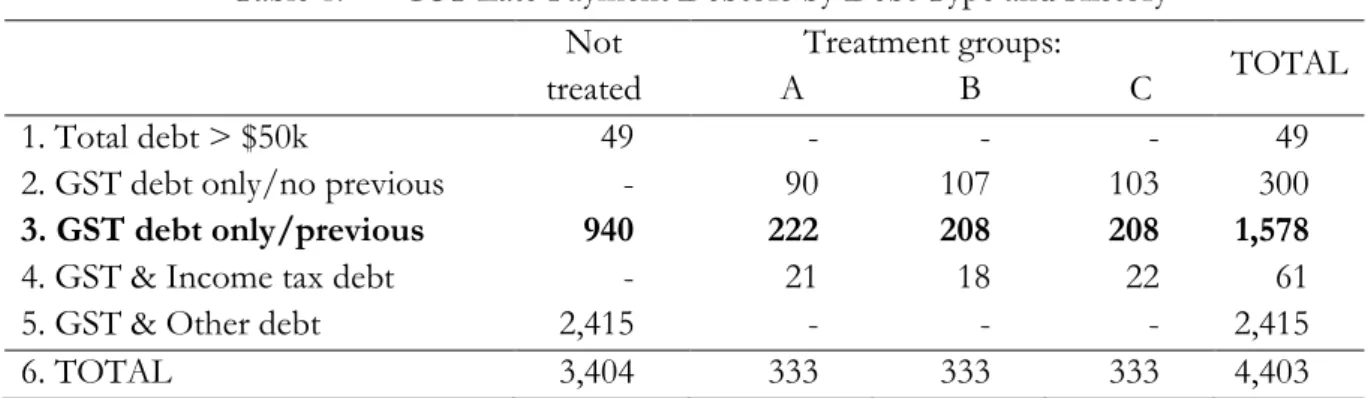
type/history as shown in Table 1. This stratification was chosen for IRD operational reasons (e.g. to focus attention on particular debtor characteristics of interest, such that the ‘treated’ included all taxpayers with both income tax and GST debt). Of course, this interferes with the random selection design, potentially limiting its usefulness as a random field experiment. Our analysis therefore proceeds by first identifying the relevant stratified taxpayer groups in Table 1, lines 1 – 5.
Table 1: GST Late Payment Debtors by Debt Type and History Not treated Treatment groups: TOTAL A B C 1. Total debt > $50k 49 - - - 49
2. GST debt only/no previous - 90 107 103 300
3. GST debt only/previous 940 222 208 208 1,578
4. GST & Income tax debt - 21 18 22 61
5. GST & Other debt 2,415 - - - 2,415
6. TOTAL 3,404 333 333 333 4,403
Line 2 shows that all of those with only GST debt, but no previous GST debt record, were selected for treatment in the intervention. A similar selection applied to the small sub-sample with both GST and income tax debt (line 4). A relatively small number of GST payers with especially large total debts (>$50,000) were also excluded from the treatment groups. We therefore focus our analysis on the 1,578 debtors in the “GST debt only, with previous GST debts” sub-sample (line 3) since their allocation was random without pre-selection. This also has the advantages of being a more homogeneous sub-sample and, having a history of GST debt, all have previous experience of the penalty regime. On the other hand, with a history of GST debt, they may be a more difficult group to induce to comply.
As noted earlier, treatment groups A, B and C were selected to receive different information on late payment penalties at the opening of the phone conversation. Group A received no penalty information before being offered an instalment arrangement (hence the instalment penalty discount was also not mentioned). Group B was first asked “did you know that you are being charged penalties on your debt to IR?”, before being told that if an instalment arrangement is entered
11
The telephone calls used in the intervention sought, at the end of the call, to obtain qualitative information on each respondent’s prior knowledge of penalties before the call. However, this was not coded, is not readily quantifiable, and may be unreliable given that (except for Group A) penalties were discussed earlier in the phone conversation.
12 An additional 30 taxpayers with 60-90 day GST debt were separately selected by IRD to receive no contact during the
into: “we’ll stop your penalties”. Groups C faced a similar conversation but received quantitative penalty information “… If you enter into an instalment arrangement, we’ll stop penalties of 1% per month from applying”.
Of most interest in the empirical analysis are groups A and C since these represent the two extremes of initiating the conversation with no penalty information, and with precise quantitative penalty information. Group B represents a less specific ‘intermediate’ penalty information set. The non-treatment group – the remaining debtors in the campaign – were also subject to increased compliance effort. However, they were not subjected to the same intensity of phone calls (to achieve contact) and were not necessarily offered an instalment arrangement. Also, some independently initiated contact with IRD during the campaign, and ‘non-treated’ conversations with IRD were not scripted to link penalty information directly with an instalment offer. Many within this non-treatment group were not successfully contacted by IRD during the campaign and hence provide a large group of ‘no response’ debtors that serve as a convenient default group in our multinomial logit analysis.
4.2 Taxpayer Responses and characteristics Data
We have information on the following taxpayer responses and characteristics:
1. Taxpayers’ initial phone responses on their intention to repay debt, obtained during the experiment’s conversations (in August-September 2014). Responses were classified as follows:
a) Immediate payment agreed
b) Instalment arrangement set-up agreed (documentation to be sent to taxpayer)
c) Postponement of decision agreed pending further communication (penalties continue) d) Miscellaneous, including unclassifiable responses
e) No response (failed to contact &/or obtain response) f) Not in debt (identified as debt cleared during the campaign)
The miscellaneous category represents a number of hard-to-classify responses including those in the treatment groups where the phone conversation proceeded in ways that prevented a clear A, B or C coding. ‘No response’ captures taxpayers with whom no successful contact was established or who were successfully contacted but from whom no response could be obtained. For the purposes of our analysis we amalgamate categories c) and d) and label as “other”. The ‘not in debt’ category are taxpayers who cleared their debt by the time the intervention succeeded in making contact with them. Since the campaign lasted approximately 2 months, numerous taxpayers paid off their debt before receiving the campaign phone call. 13 In our empirical logit
analysis below this group provide an interesting sub-sample because their payment behaviour might reasonably be regarded as not influenced by the intervention. Relative those who were not successfully contacted and who did not subsequently pay their overdue tax, the former group might be expected to display fewer non-compliance characteristics.
13 In addition a small number of taxpayers (57), indebted at the time of selection for the experiment (in May/June 2014),
were no longer indebted when the intervention began in August 2014, leaving a sample of 1,521 observations. The included ‘no longer in debt’ category refers to those who paid their GST debt during the period of the intervention but prior to being contacted by phone.
2. Taxpayers’ actual debt repayment responses (as coded by IRD) six months after the end of the experiment in March 2015. These observed outcomes were classified as follows:
(i) Immediate (within 1 month) full payment agreement is in place. (ii) Instalment arrangement is in place.
(iii) Auto-seizure action in place (i.e. following failure to obtain a voluntarily agreement, IRD is auto-seizing payment from the taxpayer’s employer or bank accounts.
(iv) Case Open: the case is unresolved – the taxpayer is considered to be ‘non-compliant’. (v) Other Action.
‘Other action’ includes cases for which debt was either cleared, or subject to an agreement to delay (e.g. due to a ‘grace period’, or ‘hardship’; hence the taxpayer is considered as ‘compliant’) or there was on-going negotiation.
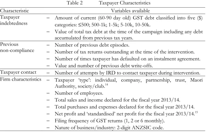
In addition, data were collected on several relevant taxpayer characteristics at the time of the intervention including levels of tax indebtedness, indicators of precious non-compliance, and other taxpayer-specific characteristics. There are listed in Table 2.
Table 2 Taxpayer Characteristics
Characteristic Variables available
Taxpayer
indebtedness −
Amount of current (60-90 day old) GST debt classified into five ($) categories: ≤500; 500-1k; 1-5k; 5-10k, 10-50k.
− Value of total tax debt at the time of the campaign including any debt accumulated from previous tax years.
Previous
non-compliance −− Number of previous debt episodes. Number of tax returns outstanding at the time of the intervention.
− Number of times taxpayer has defaulted on an instalment agreement.
− Value and number of previous debt write-offs.
Taxpayer contact − Number of attempts by IRD to contact taxpayer during intervention. Firm characteristics − Taxpayer ‘type’: individual, company, partnership, trust, Maori
Authority, society/club.14
− Number of employees.
− Total sales and income declared for the fiscal year 2013/14.
− Total purchases and expenses declared for the fiscal year 2013/14.
− Net profit and ‘standardised’ net profit for the fiscal year 2013/14.15 − Filing frequency of GST returns (1, 2 or 6 monthly).
− Nature of business/industry: 2-digit ANZSIC code. 4.3 Testing Compliance Hypothesis with Available Variables
The ASY model adapted in section 3 suggests that the taxpayer-specific perceived enforcement probability,
π
j, and borrowing costs, ρj, are expected to impact late payment/debt repayment choices in a number of ways. These subjective variables are directly unobservable but might be expected to be correlated with some of our variables available in our dataset.
14 A Māori authorities acts as a trust or company administering communally owned Māori property. 15 Firms’ profits are standardisation using the relevant industry mean and standard deviation.
For example, current debt levels should be correlated with the borrowing cost (ρj) of delayed payments, since greater amounts of debt might be expected to be associated with higher borrowing costs to repay the debt. This includes both a ‘volume effect’ (a higher amount borrowed is required) and a ‘price effect’ where larger amounts borrowed imply greater risk; hence a higher interest rate on loans. We therefore expect lower compliance – less likelihood of agreeing to repay debt – the larger is the amount of current debt.
Taxpayers’ previous non-compliance behaviour should be correlated with their perceived probability of debt enforcement,
π
j. Previous experience of non-compliance can be expected to give such taxpayers greater awareness thatπ
j. < 1. Hence the greater is previous non-compliance (e.g. more often in debt, greater the number of tax returns outstanding) the less likely is the individual to respond to an intervention with increased compliance in the form of immediate repayment or instalments. In addition greater numbers of contact attempts by IRD (before successfully making contact or failing) typically indicate that such taxpayers are harder to get hold of. Less compliant taxpayers, who are aware that avoiding/delaying contact reducesπ
j, can be expected to be disproportionately represented in this group.Similarly, taxpayers who have previously experienced more and/or higher valued debt write-offs conceded by IRD can be expected to have lower perceived probabilities of debt enforcement and hence are less likely to respond to the intervention with increased compliance.
Previous defaults on instalment agreements could affect the perceived probability of enforcement when in an instalment arrangement ( < 1). In line with the discussion proposed in section 3 we expect that the greater the number of previous defaults on instalment agreements, the more likely is a taxpayer to accept an instalment option in this case.
For firms’ characteristics, we generally do not have a priori sign predictions of their effect on compliance, but we nevertheless consider them as potentially important observable firm-level controls that can affect compliance. For example, compliance more generally is often alleged to differ by industry with some evidence that small construction sector firms, or industries dominated be self-employment entities, for example, are less compliant. Firm size measures (e.g. number of employees, earnings, profit size etc.) might be expected to be correlated with compliance if, for example, larger or more profitable firms face lower borrowing costs (via lower risk). Additionally they may be more able to reduce
π
j through resistance to enforcement efforts (e.g. via negotiations or legal procedures with IRD).For industrial sectors, in the regressions we control for the four industries where our sample is concentrated (46% of taxpayers): Construction (16.4%), Property Operators & Real Estate Services (13.8%) Professional, Scientific & Technical Services (8.3%), and Agriculture (7.7%). 4.4 Empirical Specification
To examine the role of the intervention and compliance-related factors discussed above, we examine separately the taxpayer’s declared response during the experiment, and recorded response six months later. Hence our dependent variables are declared intentions and actual behaviour six months after the period of the intervention. We group declared intentions into the five categories listed as a) to e) above, noting that c) and d) are combined. These are labelled as: ‘Pay
Now’, ‘Instalments’, ‘Other’, ‘No response’ and ‘Not in debt’. We use ‘No response’ as the base/default category in our analysis; all other declared intention categories are measured relative to this default.
We use a multinomial logistic regression model to estimate response probabilities for the five categories above of declared intention using the following four equations:
X TreatC TreatB TreatA sponse No tention DeclaredIn P PayNow tention DeclaredIn P 14 13 12 11 10 ) Re ( ) ( ln =α +α +α +α +α = = (R1) X TreatC TreatB TreatA sponse No tention DeclaredIn P s Instalment tention DeclaredIn P 24 23 22 21 20 ) Re ( ) ( ln =α +α +α +α +α = = (R2) X TreatC TreatB TreatA sponse No tention DeclaredIn P NotInDebt tention DeclaredIn P 34 33 32 31 30 ) Re ( ) ( ln =α +α +α +α +α = = (R3) X TreatC TreatB TreatA sponse No tention DeclaredIn P Other tention DeclaredIn P 44 43 42 41 40 ) Re ( ) ( ln =α +α +α +α +α = = (R4)
TreatA, TreatB and TreatC are dummy variables for treatment groups A, B and C respectively (the ‘business as usual’ group being the reference category), X is a set of control variables as described above, and the
α
’s are regression coefficients. We apply the same model to the analysis of actual behaviour, for which we consider the five categories above, namely: Pay now, Instalments, Auto-seizure, Case open and Other. Case open is our base category.By exponentiating the linear equations in (R1-R4) above we obtain the ratio of the probability of intention to ‘pay now’ (or enter instalments, etc.) to the probability of ‘no response’. These are the relative risk (odds) ratios, RRRs, shown in the tables below which provide a more straightforward interpretation. A relative risk ratio greater (less) than one implies that the likelihood of the relevant category under consideration is larger (smaller) than the likelihood of the base case. In addition the relative size of RRRs across variables and specifications indicate the relative sizes of the relevant responses.
5. Experiment Results
5.1 Declared Intentions
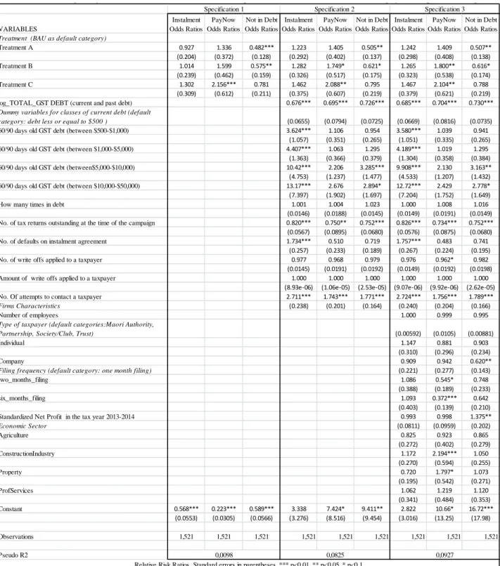
Evidence on declared intentions is presented in Table 3, showing results for two categories of intentions to repay/comply (Pay Now and Instalments) relative to the base category No Response (the least compliant).
We also include results for the category, Not in Debt. Obviously we do not expect any positive compliance effect of the experiment on this category since those taxpayers repaid their debt before they were contacted during the intervention. Nevertheless it is interesting to consider whether the ‘early’ repayment of debt by this group without the additional IRD effort is associated with particular taxpayer characteristics such as previous non-compliance, number of IRD contact attempts during the intervention, or whether some particular firm characteristics are associated with the likelihood of being in this early debt repayment category. Within our sample these represent the least non-compliant, at least in terms of the length of their payment delay.
Table 3 shows results for three specifications: specification 1 includes only the three treatment group dummy variables; specification 2 includes debt-related control variables, while specification 3 adds further firm characteristics.
All three specifications show that treatments B and C have a positive impact on the Pay Now probability, statistically significant for 5 of the 6 estimated parameters: that is, the likelihood of the taxpayer responding with an intention to pay immediately, relative to the likelihood of no response, is higher (RRR > 1) for taxpayers in treatments B and C who received penalty information/reminders. A positive effect (with lower point estimates) is also obtained for treatment group A (RRR > 1), but these are not statistically significant.
Positive effects (RRR > 1) in the treatment groups are also observed for the probability of agreeing to an instalment arrangement, but these are not statistically significant and estimated RRRs are generally lower than for the equivalent Pay Now cases across the three specifications. These results therefore suggest that, other things equal, the experimental intervention specifically targeted by IRD at groups A, B and C, succeeded in eliciting a greater intention to comply with payment of late GST liabilities, relative to non-contacted taxpayers. However, this effect appears to be associated most robustly with intentions to pay immediately (within a month) rather than to agree an instalment plan. Specifically with respect to penalty information given in the experiment, this appears to have had some effect on stated intentions to comply when mentioned to taxpayers (groups B and C), compared to those for whom no prior penalty reminders were given (group A).
In discussing the impact of control variables on payment intentions we concentrate on specification 3 which includes all controls; results are very similar for control variables that appear in both specifications 2 and 3.
Table 3 suggests that the size of taxpayers’ total debt negatively affects compliance, as expected. Before interpreting this result, recall that this sample of taxpayers only have GST debt. Therefore their total debt in this case is all GST of whatever vintage (outstanding for <60 days, 60-90 days, >90 days), whereas the intervention related specifically to the 60-90 GST debt component. The results in Table 3 however indicate that all three taxpayer intention categories which signal greater compliance (Pay Now, Instalments and Not in Debt) are less likely if taxpayers have greater total (GST) debt. We suggested earlier that such high-debt taxpayers can be expected to face higher costs of borrowing from the private sector (higher ρj) to repay tax debt. If so, ceteris paribus, they are thus less likely (than those with lower debt) to respond to the intervention by increasing compliance.
For a given size of total GST debt, higher ‘60-90day’ GST debt is expected to encourage greater compliance. This may be due to the 60-90 day specific intervention raising πj for this debt element, such that taxpayers prefer to pay off this debt rather than other tax debt they hold, and/or because the offer of a reduced instalment penalty for this GST element has greatest benefit when this element is large. As expected, Table 3 results indicate that taxpayers with greater ‘60-90 day’ GST debt are associated with being more likely to intend to enter an instalment agreement: the RRR estimates increase with the five debt size bands and are statistically significant. However, there is no significant effect on the declared intention to pay
immediately. This is consistent with the reduced penalty being a primary motivator for the increased compliance by high ‘60-90 day’ GST debtors.
More puzzling is the Table 3 result for those Not in Debt, indicating that especially large ‘60-90 day’ GST debts (>$5,000) are associated with a greater likelihood of the taxpayer being in this relatively compliant category – having paid off their late payment debt without the added incentive of the intervention.16 For those taxpayers a potential increase in πj via the intervention is irrelevant, and they did not receive an offer of an instalment arrangement for this debt. One possible reason for this result is that, with total GST debt held constant in those regressions, this variable indicates where a larger fraction of that debt is of the ‘60-90 day’ form. Hence the observation that where this fraction is high, a Not in Debt outcome is more likely may simply indicate that paying off this debt element held for a relatively short period (and hence subject to smaller penalties) involves lower costs for those taxpayers than paying off the more costly and prevalent ‘>90 day’ GST debt.
Next we consider the impact of the taxpayer’s previous record of non-compliance on their debt repayment intentions. Of the five variables listed in Table 2, we find statistically significant effects associated with two of them.17 Specifically, as expected a larger number of tax returns outstanding (not submitted to IRD), is associated with a negative impact on compliance: the greater the number of returns outstanding the less likely is a taxpayer to indicate an intention to pursue all of the three more compliant options: Pay now, Instalment, or Not in Debt, relative to the no response case.
Secondly, confirming our expectations, taxpayers with a greater number of previous defaults on an instalment agreement are statistically more likely to indicate an intention to enter an instalment agreement during the experiment, whilst reducing the likelihood of paying now (and Not in Debt – though the latter RRRs are not significantly different from one). It seems likely that this past experience of instalment defaulting by the taxpayer gives them knowledge of the system that effectively reduced their perceived probability of enforcement of such instalment arrangements, hence inducing participation in instalments, largely at the expense of immediate repayment.
None of the taxpayers’ personal characteristics is statistically significant for Instalments. Finally, other firm characteristics in general are at most weakly associated with differences in declared intentions by the taxpayer. None is statistically significant for Instalment intentions. For Pay Now intentions, less frequent filing has a negative effect, while taxpayers in two specific economic sectors (Construction, and Professional, Scientific & Technical Services) appear more likely to respond with intentions to pay immediately. There is also some evidence that firms with
16 Note that for those taxpayers, this is not a compliance intention, but actual compliance since their GST debts have
already been paid.
17 The three variable that are generally statistically insignificant are the number of times a taxpayer has previously
been in debt and the number and amount of past debt write-offs obtained, though there is some evidence in Table 3 that a greater number of past write-offs is associated with lower compliance intentions. Since taxpayers who file more often (e.g. monthly rather than 2- or 6-monthly) can have a much higher number of recorded ‘episodes’ of non-compliance or debt, and hence number of write-offs, it is possible that controlling for the filing frequency limits the regression impact of those non-compliance variables. We tested this with our data and found results did not change.
a higher standardized net profit (relative to others in their industry) are more likely to have paid their tax debt early (Not in Debt). If, as is often argued, internal sources of funds are cheaper to the firm than externally borrowed funds, this may indicate that firm-specific debt repayment costs are lower (lower ρi) when firms are more profitable.
5.2 Observed Debt Repayment Responses
Table 4 show the results for actual debt repayment behaviour, as recorded by the IRD six months after the end of the intervention, using the same three logit model specifications – with only the treatment groups (A, B, C) included in specification 1 and control variables introduced in specifications 2 and 3. Results are reported for three outcomes: Pay now, Instalments and Auto-seizure. While the former two represent increased compliance relative to the ‘No response’ category, auto-seizure represents relatively extreme non-compliance with IRD forced to sequester payment from the taxpayer’s bank.18 Comparing with results in Table 3 there is a clear difference
between taxpayers’ declared compliance intentions in response to the intervention and their subsequently observed compliance responses.
For example, being in one of the three experiment treatment groups (receiving different penalty information and reduced instalment penalties) appears to have no statistically significant effect either on the probability that a taxpayer entered an instalment arrangement, or on immediate debt repayment. Hence it would seem that any effect that the intervention’s penalty information differences had on taxpayers’ declared intentions to repay debts immediately, were not realised six months later.
Only for Auto-seizure is there evidence of significantly different effects on the treated (A, B, C) compared to the non-treated. For all three treatment groups, auto-seizure is less likely compared to the default of ‘no action’ (Case still open). This is consistent with the intervention succeeding in reducing the probability that a taxpayer is in the least compliant category (those subjected to auto-seizure). However, it may simply indicate that the IRD was less likely to pursue the auto-seizure option for the taxpayers who were in the experiment than for the non-treated group, though there was no explicit intention by IRD to differentiate between treated and no-treated taxpayer after the experiment.
The evidence on these, at most limited, actual responses by the treatment groups suggests a number of possible interpretations of the earlier evidence on taxpayers declared intentions during the experiment. Firstly, we might interpret taxpayer initial responses as a framing effect. That is, presenting taxpayers with new or repeated information on penalties generated a genuine but temporary intention to improve compliance and repay outstanding debt. However, for whatever reasons (e.g. procrastination, subsequent changes to their information sets) they failed to act consistent with increased compliance.
Secondly, treated taxpayers’ initial stated intentions to improve compliance during the experiment may have been a strategic response, for example to delay further any IRD action such as auto-seizure. If so, in the case of auto-seizure it appears to have been successful. Thirdly, this intervention involved a two-way conversation, as opposed to a letter received by the taxpayer
18 Auto-seizure of tax debt out of employee wages, via employers, is also used though in the case of GST debt this
which could be ignored. Taxpayers may therefore have felt some pressure to respond positively when contacted personally by an IRD compliance team member, even if they intended subsequently to ignore any commitments made – consistent with the way these taxpayers had responded to previous written communications from IRD.
Notwithstanding limited ‘treatment effects’ associated with penalties on actual compliance, does the evidence from control variables confirm any taxpayer-specific characteristics are associated with actual compliance behaviour?
For taxpayers who entered an instalment agreement, only one control variable appears to be statistically significant for this choice: the number of returns outstanding is associated with a negative effect (lower odds ratio) on Instalments (see specification 3). This at least is a plausible outcome – regularly non-compliant taxpayers (who persistently fail to file GST returns) are relatively unlikely to agree an instalment arrangement on their current GST debt in response to the intervention.
Of course, six months after the experiment, many of the indebted taxpayers have paid off the 60-90 day GST debt that was the focus of the intervention and are therefore recorded in the (actual) ‘Pay Now’ category.19
Table 4 indicates that a number of taxpayer characteristics increase or reduce the likelihood of paying their GST debt. Characteristics which (statistically) lower the probability of payment include:
(i) larger 60-90 day GST debt levels;
(ii) larger numbers of outstanding tax returns;
(iii) more defaults on past instalment arrangements; and
(iv) more attempts to contact the taxpayer were required in the campaign.20
Characteristics (i) – (iii) suggest plausibly that a poorer compliance record is likely to be associated with a lower probability that the taxpayer will respond positively to this compliance intervention. Characteristic (iv) is consistent with taxpayers who are more difficult to contact (perhaps by intention) also likely to be less compliant.21 Both of these effects are consistent with
the predictions from the model described earlier.
5.3 Are the Hypotheses Supported?
Section 3 suggested a number of hypotheses that could, in principle, be tested with data such as that produced by our field experiment. These hypotheses relate to the expected increase in compliance by already indebted taxpayers; that is, those already in the sub-set of taxpayers who are ‘evading’ – in this case, paying late and incurring debt. This increased compliance may occur
19 Out of a total of 179 taxpayers observed in the (actual) Pay Now category, 28 declared an intention to enter an
instalment agreement and 46 declared an intention to Pay Now. However, since over half of the total observations (787 out of 1,521) are in the ‘other’ actual category (i.e. their actual outcome is unresolved in some respect), it is possible that the limited evidence of actual compliance effects in Table 4 is partly attributable to the low number of observations whose outcomes could be analysed.
20 The table also indicates that taxpayers who have been in debt more often in the past are statistically, but
counter-intuitively, more likely to Pay Now. However with an odds ratio very close to one (1.062), any positive effect, if it exists, is very small.
21 When unable to reach a specific taxpayer by phone, IRD will typically leave a message; hence non-compliant
either through agreeing immediate debt repayment or acceptance of an offer of an instalment agreement involving lower penalties.
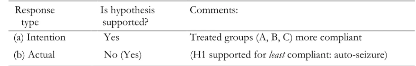
Table 5 summarises the six hypotheses and considers whether they are supported by our evidence based on (a) taxpayers stated intentions during the experiment; and (b) actual compliance outcomes after the end of it. Since these hypotheses typically relate to directly unobservable variables such as perceived probabilities and penalty rates, the ‘comments’ column in the table identifies the relevant proxy variables from our empirical results.
It can be seen that, with the exception of H6 – which cannot be tested with our available data – there is some support for each hypothesis from taxpayers’ response intentions. Based on actual improvements to compliance following the experiment there is also support for hypotheses H3 and H4. These is some, more limited, support for H1 and H5 based on evidence for some of the least compliant taxpayers in the sample (those whose tax debt was auto-seized by the revenue authority). H2 – that taxpayers with relative high borrowing costs are more likely to accept an instalment option – is not supported by actual data. However, as Figure 1 shows, taxpayers with relatively high borrowing costs are also expected to shift to immediate payment if the increase in their probability of enforcement induced by the intervention is sufficiently large. Our field experiment outcomes do provide some support for such a response, with more indebted taxpayers more likely to have paid off their debt. In this sense, a proxy for higher borrowing costs is associated with increased compliance following the enforcement intervention.
Table 5 Compliance Hypotheses and Field Experiment Outcomes
H1: Intervention (contact) raises compliance via increased perceived probability of enforcement Response
type
Is hypothesis supported?
Comments:
(a) Intention Yes Treated groups (A, B, C) more compliant
(b) Actual No (Yes) (H1 supported for least compliant: auto-seizure) H2: Taxpayers with relative high borrowing costs more likely to accept an instalment option
(a) Intention Yes Higher borrowing costs proxied by higher debt levels
(b) Actual No But higher debt levels are associated with greater
immediate repayment
H3: Taxpayers with lower perceived probability of enforcement are less likely comply
(a) Intention Yes Probability ( ) proxied by no. of outstanding returns; no. of IRD contact attempts
(b) Actual Yes
H4: Taxpayers with lower the perceived probability of enforcement of instalment agreement more likely to comply via instalments
(a) Intention Yes Probability ( ) proxied by no. of previous instalment defaults
(b) Actual No
H5: If taxpayers underestimate penalty rates, providing more accurate penalty information increases the probability that instalment, and immediate payment, options are chosen
(a) Intention Yes Greater compliance by treatment groups B & C (b) Actual No (Yes?) No greater compliance by B & C (but less
auto-seizure for B & C)
H6: The higher the proportion of the tax debt repaid as a first instalment, the lower the probability the instalment option is chosen
(a) & (b) Unable to test No data available on instalment scheduling
6. Conclusions
The ‘standard’ Allingham-Sandmo-Yitzhaki (ASY) model of tax evasion predicts effects on the extent of evasion which depend on the perceived probability of detection, the tax rate and the penalties for evasion. Despite considerable evidence on the ASY model in general, as Slemrod (2007) noted, there is very little evidence specifically on the role of penalties.
Using a field experiment involving New Zealand taxpayers’ late Goods and Service Tax (GST) payments, this paper has sought to provide evidence on the effects of late payment penalties on tax compliance. We argued that the ASY model can be applied to the late payment context by adapting it to allow for less than full enforcement of discovered evasion. It was shown that in the late payment case, the standard ASY result that evasion is optimal if the taxpayer’s expected penalty is less than one (" <1; where " is the probability of detection and is the ‘penalty rate’),22 simply becomes: < 1 + , where is the probability of enforcement and is the
taxpayer’s cost of borrowing (from the private sector) to pay overdue tax.
In testing the model using our field experiment data we sought to capture empirical proxies for the taxpayer-specific (and hard-to-observe) variables, and . In addition, especially in the context of New Zealand’s complex and relatively high penalty regime, we recognise that taxpayer awareness of the penalty rate, F, may vary, causing responses to penalties to be conditioned by the degree of awareness or salience of the penalty rate.
Our experiment involved a specific compliance intervention targeted at a random sample of around 1,500 GST payers with late payment debt owed to New Zealand’s Inland Revenue department (IRD). Selected taxpayers were contacted by phone to encourage debt repayment. Three treatment sub-groups were provided with differing degrees of information about the penalty rates applicable to their debt, and (where relevant) offered a reduced penalty rate if they entered an agreement to repay outstanding debt by instalments. Coding of taxpayers’ immediate responses allowed us to test for the impact of the intervention on intentions to pay tax. In addition, data collected after the intervention provided information on actual compliance responses.
Our empirical results suggest that differences in penalty information given to taxpayers, and reductions in penalty rates, both affect taxpayers stated intentions to comply (pay overdue tax and penalties) as predicted. For example, taxpayers given more specific information about penalties are more likely to agree to pay their tax debt immediately or to enter an instalment agreement. They are also more likely to select the instalment option where our proxies for their cost of borrowing are greater, as the adapted ASY model predicts. Likewise, a record of greater defaulting on past instalment agreements (which we hypothesised reduces their perceived
22 The ‘penalty rate’ is defined such that F > 1 and the ‘penalty rate of tax’ (for the detected non-compliant) is Ft; see
probability of enforcement for this specific arrangement) increased their likelihood of intending to adopt this option.
Analysing subsequently observed responses, however, generally suggested that taxpayers were unresponsive to penalties. Results indicated that the treatment groups, whether receiving penalty information or not, were no more or less likely to have increased their compliance (via full payment or an instalment agreement) than the non-treated. Nevertheless, a number of individual taxpayer characteristics associated with their perceived probabilities of enforcement or cost of borrowing were identifiable as affecting observed compliance by fully repaying debt. Thus for example, taxpayers with larger GST debt levels, or with a worse previous non-compliance record (greater numbers of outstanding tax returns), were found to be less likely to have become compliant by repaying their GST debt.
Finally, the results suggested some substantive differences between taxpayers’ stated intentions to comply and their subsequently observed compliance. We noted earlier that this might partly reflect the smaller numbers of taxpayers for whom actual outcomes were suitably resolved at the six month deadline when this was assessed. Nevertheless, if these intention-actual differences are genuine, at least two possible interpretations are possible (but which the field experiment, by its design, cannot resolve). Firstly, it may be that the telephone intervention (both in general and the specific presentation of penalty information) generated a framing effect whereby taxpayers were induced to respond as predicted by increasing their intention to comply. But this effect on attitudes was temporary so that taxpayers failed to follow through on their intentions. Secondly, taxpayers may have behaved strategically when faced with a person-to-person discussion with the tax authority over their tax debt. Specifically, they may have sought to gain further delay in repaying debt (hence delaying additional sanctions such as auto-seizure) by verbally agreeing to the tax authority’s suggested repayment options, even if they had little or no intention of implementing those agreements.
References
Allingham, M. G. and Sandmo, A. (1972) Income tax evasion: a theoretical analysis. Journal of Public Economics, 1, 323-338.
Gahramanov, E. (2009) The theoretical analysis of income tax evasion revisited. Economic Issues, 14, 35-41.
Kleven, H.J., Knudsen, M.B and Thustrup, C. (2011) Unwilling or unable to cheat? Evidence from a tax audit experiment in Denmark. Econometrica, 79, 651-692.
Sandmo, A. (2005) The theory of tax evasion: a retrospective view. National Tax Journal, 58, 643-663. Skov, P.E. (2013) Pay Now or Pay Later: Danish Evidence on Owed Taxes and the Impact of Small
Penalties. Working Paper, Rockwool Foundation Research Unit and University of Copenhagen. Slemrod, J. (2007) The economics of tax evasion. Journal of Economic Perspectives, 21, 25-48.
Slemrod, J., Christian, C., London, C. and Parker, J.A. (1995) April 15 syndrome. Economic Inquiry, 35, 695-709.
Yitzhaki, S. (1974) A note on: Income tax evasion: a theoretical analysis. Journal of Public Economics, 3, 201-202.