HAL Id: dumas-00981445
https://dumas.ccsd.cnrs.fr/dumas-00981445
Submitted on 22 Apr 2014HAL is a multi-disciplinary open access archive for the deposit and dissemination of sci-entific research documents, whether they are pub-lished or not. The documents may come from teaching and research institutions in France or abroad, or from public or private research centers.
L’archive ouverte pluridisciplinaire HAL, est destinée au dépôt et à la diffusion de documents scientifiques de niveau recherche, publiés ou non, émanant des établissements d’enseignement et de recherche français ou étrangers, des laboratoires publics ou privés.
Studying genetic control fo partial resistance to
Aphanomyces cochlioides (Drech) in Sugar-Beet (Beta
vulgaris L.)
Mathilde Liorzou
To cite this version:
Mathilde Liorzou. Studying genetic control fo partial resistance to Aphanomyces cochlioides (Drech) in Sugar-Beet (Beta vulgaris L.). Sciences agricoles. 2013. �dumas-00981445�
Mémoire de Fin d'Études
Diplôme d’Ingénieur de l’Institut Supérieur des Sciences Agronomiques,
Agroalimentaires, Horticoles et du Paysage
Année universitaire : 2012-2013 Spécialité : Ingénieur en Horticulture
Spécialisation : Sciences et production végétales, Amélioration des plantes
Studying genetic control of partial resistance to Aphanomyces cochlioides (Drech) in
Sugar-beet (Beta vulgaris L.)
Mathilde LIORZOU
Volet à renseigner par l’enseignant responsable de l’option/spécialisation* Bon pour dépôt (version définitive) ! ou son représentant
Date : !./!/! Signature Autorisation de diffusion : Oui ! Non!
Devant le jury : Soutenu à Rennes le 13/09/2013
Sous la présidence de : Maria Manzanares-Dauleux
Maître de stage : Stefaan Horemans
Enseignant référent : Maria Manzanares-Dauleux
Autres membres du jury (Nom, Qualité) :Mélanie Jubault et Régine Delourme
"Les analyses et les conclusions de ce travail d'étudiant n'engagent
que la responsabilité de son auteur et non celle d’AGROCAMPUS OUEST".
AGROCAMPUS OUEST CFR Angers
2 rue Le Notre 49045 Angers SESVANDERHAVE N.V. Industriepark Soldatenplein Z 2 Nr 15 3300 Tienen BELGIUM
!"#$%&'()*+($,-!
!
I would like to take this opportunity to thank all the people who have contributed in some way to my internship, particularly Stefaan Horemans, senior breeder, who initiated the project. I would like to thank him for the time and advices he gave me during my time in SESVANDERHAVE. My thanks also go to Olivier Amand who helped me a lot in my work, for his attention, and for all the time he awarded to me, his advice was really useful and appreciated.
I also thank all the members of the microbiology laboratory team who were always ready to help me. I think particularly of Erik de Bruyne, Nathalie Dupuis and Lindsey Broos. I give a particular thanks to the genetic laboratory team, who have been very helpful, especially Alexandra Burkholz and the technical staff. I am also grateful to Steve Barnes, for his advices during the redaction of my report.
Finally, I would like to thank all the members of SESVANDERHAVE "#$! %&'(! %)! "$*+! ,-&.(%(/0!12.#!&!,-(&1&/0!10&), for their warm welcome, their patience and the time they spent to explain their work to me.
Table of contents
I
NTRODUCTION... 1
B
IBLIOGRAPHY... 3
A. TAXONOMY AND BIOLOGY OF SUGAR BEET ... 3
B. APHANOMYCES COCHLIOIDES IN SUGAR BEET ... 3
1. LIFE CYCLE ... 3
2. SYMPTOMS ... 3
C. GENETICS AND GENOMICS OF SUGAR BEET ... 4
1. GENOME FACTS ... 4
2. BREEDING IN SUGAR BEET ... 4
3. BREEDING FOR DISEASE RESISTANCE ... 5
D. QUANTITATIVE TRAIT LOCI (QTL) ANALYSIS ... 7
1. QTL DEFINITION ... 7
2. PRINCIPLE OF QTL MAPPING ... 7
3. STATISTICAL METHODS FOR QTLMAPPING ... 8
4. TESTS FOR QTL SIGNIFICANCE ... 9
5. ESTIMATED PARAMETERS ... 10
6. QTL DETECTION IN SUGAR BEET ... 10
M
ATERIAL AND METHODS... 11
A. PLANT MATERIAL ... 11
1. PLANT MATERIAL USED TO DEVELOP THE BIOASSAY ... 11
2. PLANT MATERIAL USED IN REPEATING THE 2012 ASSAY ... 11
3. PLANT MATERIAL USED FOR RESISTANCE FINE MAPPING ... 11
B. SEED TREATMENT ... 11 C. INOCULUM PREPARATION ... 11 D. GROWTH CONDITIONS ... 12 1. SOWING ... 12 2. TUBE PREPARATION ... 12 3. TRANSPLANTATION ... 12 4. GROWTH CONDITIONS ... 12 5. NUTRITIVE SOLUTION ... 12 6. INOCULATION ... 12 E. EXPERIMENTAL DESIGN ... 12
F. EVALUATIONS AND ANALYSES ... 13
1. EVALUATION OF RESISTANCE ... 13 2. WATERING HOMOGENEITY ... 13 3. STATISTICAL ANALYSIS ... 13 4. QTL DETECTION ... 14
R
ESULTS... 16
A. BIOASSAY DEVELOPMENT ... 161. PATHOGEN VERIFICATION ... 16 2. HOMOGENEITY OF WATERING ... 16 C. EXPERIMENT 1 ... 17 1. STATISTICAL ANALYSIS ... 17 2. GENETIC ANALYSIS ... 17 D. EXPERIMENT 2 ... 18 1. STATISTICAL ANALYSIS ... 18 2. GENETIC ANALYSIS ... 18
D
ISCUSSION... 20
A. BIOASSAY DEVELOPMENT ... 20 B. EXPERIMENT 1 ... 21 C. EXPERIMENT 2 ... 21C
ONCLUSION... 23
LIST OF FIGURES ... 24 LIST OF TABLES ... 24ANNEXES TABLE OF CONTENTS ... 24
ABBREVIATIONS ... 24
BIBLIOGRAPHY ... 24
1
Introduction
In the current developing world, there is a need to produce more food to feed the growing population. This will require an increase in the yield of cultivated crops. Today, these yields are limited by several biotic and abiotic factors such as diseases, pests or environmental conditions.
Sugar beet (Beta vulgaris spp.vulgaris L.) is the second most important source of sugar after sugarcane, and is grown as a root crop in more than 50 countries in temperate climates. In 2011, about 270 million tons of sugar beet were produced, worldwide. The top 5 producers are France (31 million tons), USA (28 million tons), Germany (25 million tons), Russia (21 million tons) and Ukraine (18 million tons) (FAO, 2012).
SESVanderHave is an international company specialized in developing, producing and commercializing sugar beet seeds. This company exists since 2005, when the company “Maison Florimond Desprez” bought the sugar beet breeding part of Advanta seeds (which was a fusion between Zeneca seeds and VanderHave). They are continuously investing in breeding for resistance to diseases including the fungus Aphanomyces cochlioides.
The sugar beet root disease Aphanomyces cochlioides is omnipresent and causes significant yield losses mostly in the United States, in eastern and northern Europe (Metzger, et al., 2008) (Moliszewska, et al., 2008) (Piszczek, 2004) (Amein, 2006). Control of A. cochlioides has been attempted by biological, chemical, agronomic and breeding methods, but currently no really effective methods have been developed to control this disease. The most effective chemical control is Hymexazol (Tachigarin, 3-hydroxy-5-methyl-isoxazole), but its efficacy remains variable, it is expensive and is ineffective past the seedling stage (Payne, et al., 1990), (Whipps, et al., 1993), (Rush, et al., 1993). The best approach seems to be resistance breeding (Yu, 2004). Until now, only partial resistance to Aphanomyces cochlioides has been found (Bockstahler, et al., 1950).
Resistance breeding can be supported by molecular tests that may be more precise than conventional techniques. To use those molecular tests, genetic control of partial resistance to Aphanomyces cochlioides has to be found. The aim was to search for quantitative trait loci (QTL) that are potentially involved in partial resistance to Aphanomyces cochlioides. In 2012, a study was made by SESVanderHave that placed QTL for resistance on chromosomes 4 and 6 of the SESVanderHave map. The objective of the present study was to locate these more precisely and to search for flanking markers. The major problem was to evaluate and quantify resistance to A. cochlioides. Some tests already exist in the literature (Windels, et al., 1989) (Peterson, et al., 1988) (Rao, et al., 1995) (Davis, et al., 1995) (Infantino, et al., 2006) (Panella, et al., 2008). At SESVanderHave, the current screening test was based on the inhibition of plant growth related to the growth of the fungus into the root. The parameter tested was the root wet weight, but there was confusion between the inherent capacity of the plant to grow and the real effect of the disease. Therefore it has been proposed to create a new screening system based on the observation of symptoms. It has been developed on seedlings in order to get results quicker and reduce heterogeneity between plants. Several parameters have been tested such as substrate, date of inoculation or inoculum concentration. A method of scoring has also been developed. Having this method established, the assay from 2012 has been retested with the newly developed protocol to compare the obtained results with both techniques. Another set of recombinant lines has been tested to evaluate their resistance level. With the SNP (Single Nucleotide Polymorphism) marker data available, phenotypic and genotypic data have been analysed by statistical methods in order to study linkage between the data and discover loci potentially involved in the resistance; this aims to define markers linked to resistance.
2 In this report, some bibliographic information will first be summarized, to provide a better understanding of the subject. Then, material and methods will be explained, including the explanation of the screening system developed. Results will then be shown followed by a discussion.
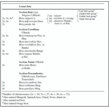
Figure 1 : Sugar beet classification (Bosemark, 2006)
Figure 2 : Phenological stages of sugar beet during the vegetative growth (ITB)
Figure 3 : Aphanomyces cochlioides (personal photography)
3
Bibliography
A. Taxonomy and biology of sugar beet
Sugar beet (Beta vulgaris) is a dicotyledonous plant belonging to the Chenopodiaceous family (Figure 1). It has a biennial cycle (UFS, 2013). It is propagated with seeds (Doré, et al., 2006).
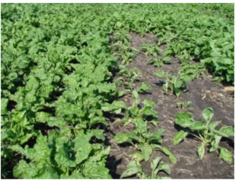
The first year of the reproduction cycle is the vegetative phase. The plant grows (Figure 2) and accumulates reserves in what we call the root, but which is actually 90% root, the upper 10% being derived from the hypocotyl (Cooke, et al., 1993). The plant reaches its final weight around October, depending on the sowing date, region! At this stage, the root can be harvested to produce sugar. This root has a truncated form and has a zone that is particularly rich in sugar named sacchariferous furrow (Doré, et al., 2006).
The optimal growth temperature is between 20 and 28°C, depending on the variety. (AgroParisTech, 2003)
B. Aphanomyces cochlioides in sugar beet
1. Life cycle
Aphanomyces cochlioides Drechsler is an oomycete water mold which causes damping-off
and root-rot diseases in Sugar beet. (Figure 3) It has a facultative necrotrophic growth habit (Garrison, 2008).
This disease occurs in all sugar beet-growing regions of the United-States, Canada, Europe and Japan. It can also cause damage on other crops like Spinacia oleracea and wild Beta spp. This contributes to the survival and increase of inoculum levels in the soil by serving as source of colonization. (Harveson, et al., 2009)
Oospores are stimulated to germinate by root exudate components including Cochliophilin A (5-hydroxy-6,7–methylenedioxyflavone, 1) (Wen, et al., 2006) when the soil is warm (22-28°C optimal) and wet. Those oospores may either form biflagellate zoospores or produce germ tubes that are capable of penetrating the tissues directly (Cerenius, et al., 1985) and infect roots. More typically, the germ tube of an oospore develops into a sporangium that produces motile zoospores (100 to 200 per sporangium (Harveson, et al., 2009)) that move through the soil water and infect roots. These zoospores can swim limited distances (<50cm) in the soil water column (Yu, 2004). In infected tissue, mycelia form sporangia and release zoospores into the soil profile or form oospores within the infected root tissues. (Figure 4)
The disease develops in light soils but development is favored in heavy-textured soils and parts of fields that tend to remain wet (Harveson, et al., 2009). A. cochlioides oospores can survive several years in soil and debris of infected weed hosts or sugar beet (Kirk, et al., 2001).
A previous study made by SESVanderHave demonstrated that the optimal temperature of growth for Aphanomyces is 28.8°C.
2. Symptoms
The fungus penetrates elongating zones of the plants that are weaker. This induces that the fungus can attack the plant from the germination and at each stage of plant development. At the seedling stage, the hypocotyl and the roots are elongating. When attacked, it causes seed-rot and damping-off. During the rest of the plant life cycle it can attack the growing roots, causing root growth reduction, sprangling (tap root
Figure 5: Damping-off (SESVANDERHAVE)
Figure 6: symptoms on older roots (SESVANDERHAVE)
4 disappearance) and sometimes plant death. All of this results in yield decreases. This is the reason why breeders are trying to create varieties that are resistant to this disease. Most of the infection occurs on older roots. Aboveground symptoms initially include undersized, non-vigorous plants with yellow leaves that wilt on hot sunny days, but recover overnight and on cool, cloudy days. Leaves can have a scorched appearance and become brittle. Severely infected plants often die. (Figures 5,6,7)
On the taproot and at the junctions with lateral roots, symptoms begin as water soaked lesions with a tan yellow color and can be superficial, turning light to medium brown as they dry. These lesions can result in stunting of the root as well as rotting of the root tip and sometimes in shriveled vascular tissue. This latter syndrome is known as taproot tip rot. Infection on younger plants may induce the excessive production of lateral roots. This reaction allows the plant to compensate for the loss of a root tip and can be confused with symptoms of rhizomania. In severe cases, the disease can destroy most of the taproot. (Harveson, et al., 2009)
Roots with active or inactive infections show reduced yield and sucrose content and higher levels of impurities (non-sucrose constituents), which make sucrose extraction difficult and expensive. Aphanomyces cochlioides also negatively affects the storability of sugar beet roots (Harveson, et al., 2009).
C. Genetics and genomics of sugar beet
1. Genome facts
Sugar beet has a genome of nine chromosomes. It is diploid at the natural stage (n=9), but it also exist some artificial polyploïds that are used in breeding programs (Yu, 2004). The total genome size is 758 million basepairs (Mbp) per haploid genome, varying between different sub-species (Arumuganathan, et al., 1991), (Schmidt, et al., 1998). Herwig et al. (Herwig, et al., 2002) estimated at 25 000 the number of different genes in sugar beet genome. Numerous genetic maps have been made with different types of molecular marker:
- RFLP, restriction fragment length polymorphisms (Barzen, et al., 1992), (Barzen, et al., 1995), (Pillen, et al., 1992)
- RAPD, randomly amplified polymorphic DNA (Barzen, et al., 1995)
- AFLP, amplified fragment length polymorphisms (Schondelmaier, et al., 1996) - SSR, simple sequence repeats (Rae, et al., 2000)
- SNP, single nucleotide polymorphisms (Möhring, et al., 2004), (Schneider, et al., 2007) They usually show nine linkage groups
The physical map of sugar beet was published on the 14th February 2012 (Dohm, et al., 2012). This was the result of a sequencing work done by several companies and laboratories. Because these results were not entirely public, SESVanderHave has to make its own sequence with its own markers.
2. Breeding in sugar beet
Genetic variation of sugar beet is thought to be limited since it was selected from white fodder beet (Yu, 2004). However, it has a short breeding history because it started to be selected in the 18th century (Achard, 1803) (in comparison to wheat which has been selected since 14 000 years). Moreover, this plant has long cycles of two years thus the process of selection is slowed down. Annual progress in yield is above 1% per year (Zimmermann, et al., 2000).
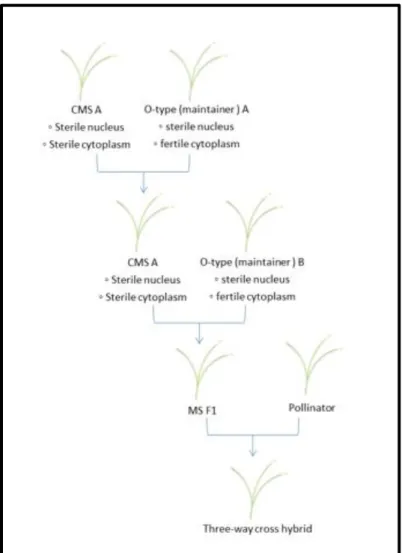
5 Because sugar beet is an allogamous plant, hybrids can be easily made and their vigor can be used. At first, hybrids were made randomly, then their production was more organized. Using tetraploids, breeding companies could make triploid plants that could not be multiplied by farmers. In the 50’s, monogermy and male sterility were discovered both in a low yielding female plant (Biancardi, et al., 2004). Initially tetraploid plants could be crossed with this female and form strong hybrids because two chromosomes out of three were coming from the male. Current sugar beet hybrids are mostly, if not all, diploid. Male sterile lines are produced with the help of maintainers plant (known as O-types) which carry the same sterility genes as the male sterile but in normal cytoplasm (they are equivalent). Female plant of an hybrid is usually an hybrid of a CMS with another non-equivalent O-type. The hybrid produced is a three-way cross hybrid. (figure 8) Progress in male plant breeding is faster and easier but progress in the female plant breeding has a larger room for progress because they were less selected until now.
Hybridization with Beta maritima or B. vulgaris and artificial hybridization with B.
procumbens or B. webbiana can be sources of new traits (Biancardi, et al., 2011).
The objectives of sugar beet breeding programs are to create stable, reliable varieties that have the highest possible yield of sugar per unit area in relation to cost of production, and that meet other requirements of the environment, growers and sugar factories (Bosemark, 2006).
Among the breeding traits, the most important are seed quality (germination rate, monogermy), sugar yield (from 3,5 t/ha in 1946 to about 13 t/ha in 2011 (Desprez, 2013)), industrial quality (sugar content, ratio sugar molasses/sugar content, low impurities content), decrease of soil tare level (soil which sticks to the sacchariferous furrow), decrease of nitrogen needs.
However, because there is almost always a negative correlation between root yield and sugar percentage, maximum expression of both characters is difficult to obtain in the same genotype. Moreover, to produce the high and stable yields required today, sugar beet cultivars must have resistance or tolerance to important pests and diseases such as Rhizomania, Nematodes, Rhizoctonia, Cercospora, and curly top. Similarly, to counter effects of possible climatic changes in the year ahead, breeders may soon have to breed for tolerance to drought or other climatic or edaphic stress factors (Bosemark, 2006).
3. Breeding for disease resistance
a. What is resistance?
Pressured by the presence of a pathogen, plants react differently. They can be susceptible or resistant. Two types of resistance exist, vertical or horizontal. Vertical resistance is generally total and specific to one isolate. It triggers a hypersensitive response like apoptosis. It is based upon one or a few major genes. It is easy and quick to use. However, there is a high risk of collapse of the resistance; this is called the ‘vertifolia’ effect.
Horizontal resistance is partial and its effect is more to slow down the infection with some barriers rather than to stop it completely. It is a polygenic resistance with several minor genes. The major advantage is that it is a stable resistance. On the other hand, the transfer is slow and difficult and the genetic background can play a key role. (personal communication M. Meulemans, 2013, (Lepoivre, 2003))
b. Resistance to Aphanomyces cochlioides
The best approach to control Aphanomyces cochlioides seems to be resistance breeding (Yu, 2004). However, the genetic mechanism of resistance is poorly understood
6 (Campbell, et al., 1993) and Aphanomyces is the disease for which least progress has been made, because of the lack of highly resistant sources and the difficulty of creating reproducible Aphanomyces infections for lab or field screening (Yu, 2004). A lot of varieties were tested for resistance (Afanasiev, 1956) (Schneider, et al., 1961), but none was highly resistant and most were susceptible. The fact that it is a very unpredictable disease makes it more difficult to study. It needs an association of several environmental conditions that does not occur every year.
However, partial genetic resistance to Aphanomyces has been described for over 50 years. Although it was shown that resistance to Aphanomyces was heritable and dominant, inheritance of resistance is poorly understood (Bockstahler, et al., 1950).
Lines with resistance to Aphanomyces have primarily been developed in East Lansing, MI, and several breeding lines (US-H20, EL48 and SP6822 for instance) were derived from selections made under high disease pressure (Yu, 2004), in naturally infested fields. Resistance was measured by harvest yield as an indirect measure of the persistence of sugar beet stands after infection earlier in the season. Greenhouse evaluations were generally found to reflect field performance (Schneider 1954, 1959). Correlations were however inconsistent (Schneider, et al., 1983) presumably due to the difficulty to control variables such as effective inoculum concentration, and to variability in soil conditions (Yu, 2004).
Breeding sugar beet resistance to Aphanomyces at both the seedling and plant stages remains an important breeding objective. It will reduce not only production costs but also the potential pollution caused by fungicide application. However, resistance sources are limited: the genetic background of the resistance seems to be narrow, with no more than a few germplasm sources (Yu, 2004).
Another problem for the study of resistance to Aphanomyces cochlioides is the lack of a reliable resistance test. Most of them are based on varieties’ yield performance in the field with Aphanomyces cochlioides epidemics, but reproducibility is low due to interference from many environmental factors (Downie, et al., 1952).
c. Bioassay
A good bioassay should be reliable. Results have to be correlated with what is found in the field and repeatable. A number of factors have to be determined: culture conditions (container, substrate, time of inoculation, culture temperature, water need!), quantifying method (visual, coloration, fluorescence, molecular techniques!), material used (should be discriminant).
d. Techniques of existing bioassays
Inoculum production
Both oospores and zoospores have been used for artificial inoculation of sugar beet seedlings (Coe, et al., 1966), (Schneider, 1954), (Schneider, 1978), (Schneider, et al., 1983). Oospores have the advantage that they can be produced easily, and can be maintained in long term storage. However their disadvantage is that the timing of inoculation of very young seedlings (<2 weeks old) introduces a time lag between oospore germination, zoospore release, infection, ramification and development of symptoms. Zoospores have the advantage of being abundant and easily produced, but the disadvantage of rapidly encysting in adverse conditions (agitation, light, presence of polyvalent cations!).This reduces the effective concentration of active zoospores presented to the seedling. Resistant and susceptible varieties could be discriminated reliably using active zoospores as the inoculum. (Yu, 2004)
7 Scoring
Most of the bioassays are performed on adult plants and scoring is made on roots (Peterson, et al., 1988), (Rao, et al., 1995), (Davis, et al., 1995), (Infantino, et al., 2006), (Beale, et al., 2002), (Metzger, et al., 2008), (Moliszewska, et al., 2008). Plant can also be scored upon their general appearance (Panella, et al., 2008) (Grünwald, et al., 2003) (Pilet-Nayel, et al., 2002) (Davis, et al., 1995).
A few bioassays with Aphanomyces cochlioides have been performed on seedlings. Coe & Schneider (1966) chose to compute a mean disease severity index of different entries by assigning a numerical rating to each surviving plant according to severity of symptoms, totaling the individual plant scores and dividing it by the number of plants inoculated. They also made a numerical rating expressing the foliage vigor of the surviving plants assigned to each entry. Results from the two methods generally correlated well with one another. Some other technics could be used to avoid a biased score, but they first have to be tested. Thermography and chlorophyll-fluorescence imaging can show a change in photosynthetic efficiency and transpiration (Chaerle, et al., 2004). Real time PCR methods are currently gaining interest. PCR can measure the correlation between amount of pathogen DNA and the reaction of the cultivar (Infantino, et al., 2006), (Weiland, et al., 2000). This method is sensitive enough to detect pathogen in symptomless tissues (Okubara, et al., 2005). SESVanderHave already used real time PCR for cercospora leaf spot detection and it was effective (De Coninck, et al., 2012).
D. Quantitative Trait Loci (QTL) analysis
1. QTL definition
Nowadays molecular tools and statistical methods allow to localize genes implied in quantitative resistance on genetic maps and to estimate their effect. They are called QTL for “quantitative trait loci”. QTL are generally spread all over the plant genome. A lot of factors can influence the detection (type and size of the segregating population, detection threshold, heritability, phenotype measurement, map accuracy!). (Kover, et al., 2001).
2. Principle of QTL mapping
a. Principle
QTL mapping is a statistical study of the alleles that occurs at a locus and the phenotypes that they produce. It is based on the segregation of genes and markers via chromosome recombination during the meiosis, thus allowing their analysis in the progeny (Paterson, 1996).
QTL analysis depends on linkage disequilibrium (LD), a situation where genes fail to segregate independently between genetic markers and the QTL. Two main analyses exist: linkage analysis and association analysis. They differ on the type of population used. Different statistical approaches can be used to detect the most likely positions of QTL: simple regression, interval mapping, composite interval mapping and a stepwise approach. These approaches allow the detection of interactions between QTL.
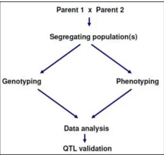
Several steps are necessary in a QTL mapping study (Figure 9). First, parents have to be chosen in order to produce a segregating population. Then this population should be both genotyped and phenotyped, and the data combined to detect and quantify a QTL.
b. Requirements for QTL mapping
Type and size of mapping population. The mapping population should use parental lines that are contrasting phenotypically for the target trait. They should be genetically
8 divergent, to permit the identification of a large set of polymorphic markers that are well distributed across the genome. The choice of mapping population (F2, Double Haploid,
Recombinant Inbred Lines!) can vary, depending on the objectives of the experiment. The size of mapping population for QTL analysis depends on several factors (Buerstmayr, 2011).
Saturated linkage map based on molecular markers. To perform a whole-genome QTL scan, it is desirable to have a complete coverage of the genome under investigation. In such a map, markers are available on each chromosome from one end to the other, and adjacent markers are sufficiently close that recombination events only rarely occur between them. For practical purposes, it is generally required to have a map distance of about 5 to 10 centiMorgans (cM). To be useful, markers should be polymorphic in the mapping population (Prasanna, 2003) (Buerstmayr, 2011).
Reliable phenotypic screening of mapping population. This is the critical part of the analysis. This screening has to be as precise as possible. Basic phenotypic data are the estimates of phenotypic performance of individuals across environments. The accuracy and precision of phenotyping determines how realistic the QTL mapping results are. An appropriate phenotyping protocol should consist of a representative sample of environments and their optimal location; a number of replications per individual in each environment; an experimental design: randomization provides statistical validity to results and protection from bias. However, there is always some variation left uncontrolled within blocks.
3. Statistical methods for QTL Mapping
a. Analysis of variance (ANOVA)
This method is the simplest (Soller, et al., 1976). The aim is to test the H0 hypothesis for each marker: “there is no difference in the mean of the trait between lines that possess marker allele A from lines that possess the alternative allele B”. This hypothesis is tested using t-tests or F-tests (Prasanna, 2003).
This method gives an approximate QTL position, a statistical significance (p-value), a percentage of phenotypic variance explained by each marker and an estimate of additive and dominant effects of single QTL. However, it has some disadvantages because it does not include the map information and each marker is treated as an independent statistical test (Buerstmayr, 2011). It is also difficult to conduct separate estimates of QTL location and QTL effect. A weak QTL effect near the marker can be confused with strong QTL effects far from the marker. Moreover, individuals with missing genotypes often need to be discarded. Last, when the markers are widely spaced and/or unevenly distributed, the QTL may be quite far from neighboring markers, and hence the power for QTL detection will decrease (Lander, et al., 1989), (Manly, et al., April 1999), (Broman, 2001).
The rank sum test of Kruskal Wallis can be regarded as the nonparametric equivalent of the one way analysis of variance. With this test, no assumptions are made about the probability distribution of the quantitative trait. (Van Ooijen, 2009)
b. Interval mapping method
Simple Interval Mapping (SIM). This method developed by Lander et al. (1989) includes the genetic map information. The aim is to test the likelihood that a QTL could occur at certain intervals along the genetic map. This is done by performing a likelihood ratio test at every position within the interval. In this approach, the QTL is located within a chromosomal interval, defined by the flanking markers. (Lander, et al., 1989) proposed a simple rule for constructing confidence intervals for QTL position, which uses the logarithm of odds (LOD score).
9 LOD score is defined as the logarithm of the ratio of two likelihoods: the likelihood for the alternative hypothesis (that there is a QTL) and the likelihood of the null hypothesis (that there is no QTL). A LOD score of three for a given point means the odds are a thousand to one in favor of a QTL being located at that position (Buerstmayr, 2011).
SIM has more power and requires fewer individuals than ANOVA (Lander, et al., 1989), (Knott, et al., 1992), (Zeng, 1994) but it has limitations. First, SIM considers one QTL at a time, ignoring the effects of other (mapped or not yet mapped) QTL. Therefore, SIM can provide a biased identification and estimation of the effect and position of QTL when such multiple QTL are located in the same linkage group (Knott, et al., 1992), (Martinez, et al., 1992), (Zeng, 1994). Second, QTL outside the interval under consideration can affect the ability to find a QTL within it (Zeng, 1994). Third, false identification of a QTL (false positive) can arise if other QTL are linked to the interval of interest.
Composite Interval Mapping (CIM). (Jansen, 1993), (Zeng, 1993) and (Zeng, 1994). It is an expansion of SIM. Markers near the QTL are included as cofactors in the estimation of QTL effects. This minimizes the effects of QTL in the remaining genome when attempting to identify a QTL in a particular region. It increases the power of detection for weak effects’ QTL that can be hidden by a QTL of strong effect.
It has the advantage of giving a more precise estimation of the QTL position. This is especially useful when QTL are close to each other in the same linkage group. It must be used carefully because it can lead to calculation artifacts (Buerstmayr, 2011). CIM can be affected by an uneven distribution of markers in the genome, and is not directly extendable to analyze epistasis. The use of tightly linked markers as cofactors can reduce the statistical power to detect a QTL (Zeng, et al., 1999).
Multiple Interval Mapping (MIM). To avoid CIM’s limitations, (Kao, et al., 1999) proposed an implemented “multiple interval mapping” (MIM) to map multiple QTL simultaneously. The idea of MIM is to fit multiple putative QTL effects and associated epistatic effects directly in a model to facilitate the search, test and estimation of positions, effects and interactions of multiple QTL. MIM consists of an evaluation procedure designed to analyze the likelihood of the data given a genetic model (number, positions and epistatic terms of QTL). When compared with methods such as SIM and CIM, MIM tends to be more powerful and precise in detecting QTL.
4. Tests for QTL significance
One of the challenges for QTL mapping is the difficulty of determining appropriate significance thresholds (critical values) for the two types of errors: false positive and false negative. Determining appropriate threshold values appears to be difficult because many factors can vary between two experiments and can influence the distribution of the test statistics. These include, but are not limited to, the sample size, the genetic map density, segregation ratio distortions, the proportion of missing data. A permutation test is usually used to determine a threshold value for significance testing of the existence of a QTL effect. Permutation tests generate many different samples from the actual data by randomizing trait values with respect to the marker genotypes to estimate empirically the threshold for a test statistic for detection of a QTL. This approach accounts for missing marker data, actual marker densities, and nonrandom segregation of marker alleles. This permutation analysis is repeated for a number of replicates (usually 1,000 permutations) to obtain a distribution of the maximum test statistics, and from the distribution to obtain the threshold value (Semagn, et al., 2010).
10 5. Estimated parameters
a. Confidence interval
Lander et al. (1989) suggested to find the location of the estimated QTL using a decrease of one from the peak LOD score.
b. QTL effect
The additive effect represents half of the difference between the averages of both parental alleles in segregation. This effect is expressed in the units of the trait being studied. It has a meaning in reference to one of two parents arbitrarily chosen. In addition, the QTL effect is also estimated by the percentage of the phenotypic variation explained by the QTL.
6. QTL detection in Sugar Beet
In sugar beet, several QTL have been mapped for sucrose yield and quality, yield and some qualitative traits (as nitrogen, potassium...) (Schneider, et al., 2002) (Möhring, et al., 2004), restoration of CMS (Hjerdin-Panagopoulos, et al., 2002), disease resistances (Cercospora leaf spot (Setiawan, et al., 2000), Rhizoctonia root and Rhizoctonia solani). A previous study made by SESVanderHave showed that resistance for Aphanomyces
Table 1 : Genotype of the parents for experiment 1
Figure 10 : Genetic map of the used markers
Figure 11: Genealogy of the tested populations
!"
"
#" ""
$" %&'(")*"+,-+" .'/'&/'(")*"/0'"&/1(2" %&'(")*"/0'"3)*'"4566)*7" 5&&52" 8'93)*7" A 0 6 9 _ S 0 1 8 A 0 8 2 _ S 0 2 15 A 0 8 7 _ S 0 2 18 A 0 9 6 _ S 0 1 20 A 0 2 8 _ S 0 2 28 A 0 4 6 _ S 0 2 34 A 0 2 5 _ S 0 2 38 A 0 5 1 _ S 0 1 40 A 0 6 2 _ S 0 2 A 0 6 2 _ S 0 1 50 A 0 6 8 _ S 0 1 59 A 0 3 9 _ S 0 1 66 C1 D15 6 _ S 0 1 -2 D07 5 _ S 0 1 0 D16 1 _ S 0 1 3 D16 8 _ S 0 1 10 D06 9 _ S 0 1 14 D18 3 _ S 0 1 20 D07 7 _ S 0 2 24 D20 1 _ S 0 1 30 D09 3 _ S 0 2 36 D10 1 _ S 0 1 38 D02 8 _ S 0 2 41 D04 5 _ S 0 7 43 D08 4 _ S 0 1 44 D13 6 _ S 0 1 45 D10 2 _ S 0 3 46 D10 6 _ S 0 1 D10 6 _ S 0 3 49 D12 2 _ S 0 1 70 D10 7 _ S 0 1 76 D10 5 _ S 0 1 86 C4 F08 6 _ S 0 4 8 F08 5 _ S 0 1 9 F10 7 _ S 0 1 18 F06 7 _ S 0 3 24 F09 6 _ S 0 1 F10 8 _ S 0 1 25 F03 6 _ S 0 1 F06 5 _ S 0 2 29 F13 0 _ S 0 1 35 F13 2 _ S 0 1 37 F11 8 _ S 0 1 40 F03 9 _ S 0 1 42 F07 2 _ S 0 1 45 F03 5 _ S 0 1 70 F07 3 _ S 0 1 82 C611
Material and methods
A. Plant material
1. Plant material used to develop the bioassay
The sugar beet lines that have been used for this work were, a line derived from FC607 (abbreviated in the text as FC607), DKPP and their hybrid FC607xDKPP. FC607 is the resistance source and is derived from an American line (Smith, 1980). It is partially resistant to Aphanomyces cochlioides. DKPP is an elite pollinator line, susceptible to
Aphanomyces cochlioides and is a multigerm line.
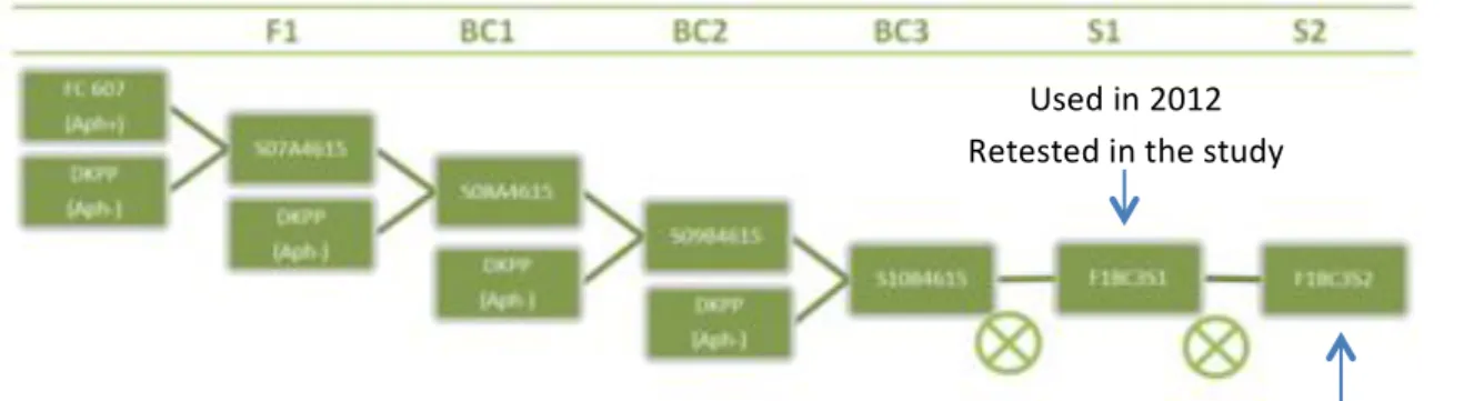
2. Plant material used in repeating the 2012 assay
Plant material used in the 2012 assay came from an initial cross between FC607 and DKPP. It was a BC3 S1 level (three backcrosses with DKPP as a recurrent parent and one selfing). The genealogy is shown in figure 11. This population was called artificial because those lines were selected for their variability for the resistance character (it was not following the Hardy-Weinberg principle). 16 lines were tested and segregate for the chromosomal region which was expected to carry the character. Three groups of genotypes could be outlined. One which was entirely heterozygous on chromosome 4 (between 38 and 57 cM) (group A), one which was heterozygous between 38 and 49 cM (group B), and the last which was heterozygous between 38 and 41 cM (group C).(Table 1)
Chromosomes were all fixed except chromosomes 1, 4 and 6. (Figure 10)
Three controls have been used, and were the same as those used to develop the bioassay : FC607, DKPP and their hybrid.
3. Plant material used for resistance fine mapping
The lines used here were BC3 S2 lines. They were the product of the same initial cross between FC607 and DKPP than the previous assay with one more selfing (Figure 11). DKPP was the recurrent parent. As it was a backcross line, that meant that some parts of the chromosomes were still unfixed. Because it descended from the previous population, it is also an artificial one.
As it was supposed that QTL for resistance were situated on chromosomes 4 and 6 from a previous bioassay, these parts of the genome were particularly selected during the backcrosses to keep variability in those zones. Among all families, 16 were selected, depending on their genotype. It should allow a good coverage of recombination events to locate the resistance more precisely. We focused here on the 20 to 50 cM zone of chromosome 4. (Figure 12)
The same controls as the previous assay were used.
B. Seed treatment
After the harvest, seeds were dried in a room at 29°C for 3 to 4 days. Then they were cleaned, and dust and small seeds were removed. Before using it in an assay, to prevent them from being already infected with Aphanomyces cochlioides or another fungi, seeds were washed with water during 4 hours. A fungicide could not be used to avoid interference with future inoculation.
Figure 12 : Genotype of the parents for fine mapping assay
12
C. Inoculum preparation
Aphanomyces cochlioides was isolated and cultivated on a potato dextrose agar (PDA)
medium for 7 days at 24°C. Spores were then cultured in a maltose dextrose solution for 5 days at 24°C. Then they were washed 3 times with autoclaved mineral water of the Spa brand. On the last day, a sample of the solution was diluted 100-fold and the spores were counted to determine their concentration. During the inoculum preparation time the solution was shaken but not too strongly to avoid damage to the flagella. According to the number of spores in the solution, they were diluted to reach the desired concentration. The precise protocol used was the same as the one which is usually used by SESVanderHave. A mixture of several Aphanomyces cochlioides strains were used for this assay. They all came from strains produced by the lab.
D. Growth conditions
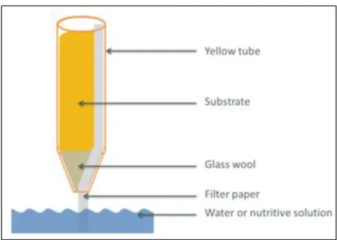
During the development of the bioassay, different growth conditions were tested: different growth systems (in tubes or in trays, with compost or with sand), different dates of inoculation and different inoculum concentrations. More information about material and methods used to develop the bioassay can be found in annexes I and II. At the end of the development, it has been decided to keep the following protocol using tubes.(Figure 13)
1. Sowing
Seeds were placed in a box containing an accordion-shaped filter paper. Then 38 mL of water were added into the box. First they were put to germinate in the dark in an incubator at 24°C during 3 to 4 days. Then they were put under light in a growth chamber at 18°C during the day (16h light period) and 19°C at night (8h) for 2 to 3 days.
2. Tube preparation
Tubes (about 20 cm long and 2 cm in diameter) were filled with sand. At the bottom of it, a piece of glass wool was placed to block the holes. A capillary matting strip was placed from the top to the bottom (through the piece of glass wool) to irrigate the substrate (Figure 14). 2 days before transplantation, the tubes were placed in a water box to humidify the sand.
3. Transplantation
Six and seven days after sowing, plants were transplanted into the sand. 10 mL of water was added to each plant at this stage to ensure that the plants were well watered from the beginning.
4. Growth conditions
Plants were then placed in a growth chamber (phytotron) at a temperature of 22°C in the day (16h) and 19°C in the night (8h). Those temperatures were chosen as being optimal for the growth of the sugar beet and the pathogen.
Two days after transplanting, plants were irrigated with nutritive solution. 5. Nutritive solution
The nutritive solution used here was the Steiner solution (see annex II) diluted 10 times. 6. Inoculation
Plants were inoculated 22 days after sowing. 1ml of 2000sp/ml inoculum solution was applied at the bottom of the hypocotyl using a pipette. Care was taken that all plants were well watered prior to infection.
Figure 13 : Protocol’s steps followed for the experiments
13
E. Experimental design
In the phytotron where the test was performed, no gradient (temperature, light!) was observed. It could have been easy to make only one randomized complete block. However, 600 plants had to be cultivated and the boxes can just contain 200, so three blocks were still needed. In each block, there were 10 repetitions of each genotype. This make in total 30 repetitions per genotype, except for DKPP which had 20 repetitions in each block or 60 repetitions in total. All repetitions were randomized in the block.
To make it easier, in the rest of the document the repeat of the assay made in 2012 will be called “experiment 1” and the assay for fine mapping will be referred as “experiment 2”
F. Evaluations and analyses
1. Evaluation of resistance
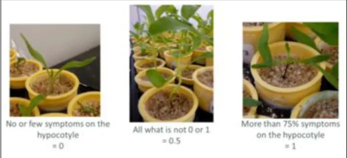
A first type of scoring was made during the incubation based on the example used by Yu (2004). The score “0” meant that plant had no or a few symptoms. The score ”1” meant that more than 2/3 of hypocotyl and root surface was diseased. “0,5” was used for all other cases which were not 0 nor 1 (Figure 15).
During the bioassay development, on the final scoring day (around 16 days after inoculation) additional evaluations were performed.
Root observations
Root were cut under the hypocotyl and the weight was measured. Statistical analysis on the data were made, but the results were not consistent. The idea came to observe the roots and calculate the infected surface with the help of a software used in an assay for nematodes. But after the first trial, it was noticed that plants were too young and roots were too thin to see anything on it.
qPCR trials
After weighing, root samples were prepared in order to perform a qPCR assessing the quantity of Aphanomyces DNA in comparison with the quantity of sugar beet DNA.
The samples were washed to remove remaining substrate, they were put in a 96-well box and put, at least one hour, at -80°C. Then, the samples were put in the freeze-dryer during two days. The dryed samples were then grinded. The DNA was extracted with the kit usually used by SESVanderHave, “Nucleomag 96 plant” from Macherey Nagel.. The qPCR is made with specific primers adapted to Aphanomyces cochlioides and sugar beet. The PCR technic used is the TaqMan.
The results given were the cycle threshold (Ct) of each sample for both sugar-beet and
Aphanomyces cochlioides. With those data it was possible to calculate the 2-""Ct which is a
common value used to quantify DNA in qPCR. An mean comparison with the Duncan test allowed to compare the three genotypes (controls) used.
Due to bad results for the bioassay development, those evaluations were not executed for experiment 1 and 2.
Pathogen identification
To be sure that the plants were really inoculated with Aphanomyces cochlioides a part from an infected hypocotyl was isolated on PDA. A few days later, it was possible to recognize Aphanomyces cochlioides under a microscope (Figure 3).
14 2. Watering homogeneity
To evaluate if water was homogeneously distributed in the tubes, they were weighed before and after watering. Two repetitions were made, one for each assay.
3. Statistical analysis
Statistical analyses were made with the software R ( R Core Team, 2013). Statistical analyses were made on all the data to assess significant differences between treatments.
a. Analyses of variance
Because this study involved different scoring time points, it was possible to do a kinetic analysis by the mean of the evaluation of the AUDPC (Area Under Disease Progression Curve). AUDPC was calculated from the first day after inoculation until the last day of the experimentation (19dpi for experiment 1 and 15dpi for experiment 2). Besides the AUDPC value, the score at the day were the controls are the most significantly different from one another and where the range between the most susceptible and the most resistant is the maximal was chosen as a second score (it was 7dpi for both experiment).
The evaluation of different effects on 7dpi score and AUDPC was made by an ANOVA. The analysis of variance model was the following: AUDPCij = µ + gi + !j +". AUDPCij is the AUDPC of genotype i in block j, µ is the AUDPC mean, gi is the genotype effect, !j is the block effect and " the residuals effects. Respectively for 7dpi: 7dpiij = µ + gi + !j +".
b. Mean comparison
This ANOVA was followed by a Duncan test to make groups with individuals that are not significantly different from each other. To be more precise, a Dunnett test allowed to compare all genotypes to each controls.
As no block effects were detected in either of the assays, there was no need to adjust the individual values.
c. Heritability
Heritability was calculated with ANOVA data with the following formula: With #$g as the genetic variance, #$e as the residual variance and n the number of repetitions per tested lines.
d. Individual distribution
Individuals’ distributions were represented according to the individuals’ response to
Aphanomyces cochlioides infection.
4. QTL detection
The analyses were made with the MapQTL6 software (Van Ooijen, 2009).
a. Genotyping
For the experiment 1 and 2, remaining leaves were sampled to allow genotyping. For experiment 1, only leaves that were still healthy at the end of the experiment were sampled, for experiment 2, as much leaf material as possible were sampled during the assay, as soon as plants have a score of “1”.
In this study, SESVanderHave consensus map was used. Markers that were chosen in this study have a segregating genotype at their locus.
At each marker, the genotype “A” was given to plants having the genotype coming from FC607 (Resistance donor plant) and le genotype “B” was given to plants whose genotype come from DKPP (receiver plant). “H” was given to heterozygous plants.
! " # $ % & + = n e g g h 2 2 2 2 ' ' '
15
b. Experiment 1
This analysis was made with 16 markers SNP (on chromosomes 4 and 6) with a segregating population of 16 lines (total of 182 individuals sampled).
Comparison of the three genotypes groups
To compare those three groups, the ANOVA model: Groupi = µ + Gi +! was followed. Groupij is the Group named i, µ is the group mean, Gi is the group effect and ! the residuals effects.
Rank sum test of Kruskal-Wallis
Because our population has a non-normal distribution, Kruskal-Wallis test was preferred to ANOVA. No further analysis will be made because this population is not adapted for QTL mapping.
c. Experiment 2
The analysis was made with 53 markers SNP (on chromosomes 1, 4 and 6) with a segregating population of 16 lines (total of 262 individuals sampled).
Comparison of families results
As a first overview of the results, results of each individual were observed. For each, a letter was given: “A” if the scores (7dpi score and AUDPC) were low and seem to show resistance (usually 0 for 7dpi score and less than 11 for the AUDPC), “B” if they are high (usually 1 for 7dpi score and more than 16 for AUDPC) and seems to be susceptible. “H” is for all other cases. In each family, for each letter, the number of individuals was counted and the mean was calculated. Looking at the family results, it is possible to give the same letters to the global family. “A” is given when the family has a lot of “A” and “H” individuals compared to “B”, “B” is given when the family has a lot of “B” individuals compared to “A” and “H” and “H” is given for all intermediate families.
With those results in parallel to the genotype data, it might be possible to see a tendency in marker alleles of genotypes that are more resistant.
Rank sum test of Kruskal-Wallis
Like for experiment 1, a Kruskal-Wallis test was made on the data. Interval mapping
This analysis was made for both traits, 7dpi score and AUDPC. It was made only on chromosomes 1, 4 and 6. For each family, parts that were fixed were treated as missing data otherwise it could have disturbed the analysis.
Because the population used here is an artificial one, it was not possible to make a special map for this assay, this is why the consensus map from SESVanderHave was used.
LOD score
To know if the results are significant, the maximum LOD score was calculated using a permutation test with 1000 iterations. The genome wide threshold with a P-value of 0.05 (or 5%) was chosen. Genome wide means that it is the maximum LOD value everywhere in the genome including all linkage groups.
MQM (Multiple QTL Mapping)
This analyze was done in the same way as interval mapping, except that some co-factors were manually selected. They were chosen on results obtained in the interval mapping test.
Figure 16: Assay with different inoculation dates
Figure 17 : assay with different inoculum concentrations
Figure 18 : last assay confirming the two previous assays and qPCR results
16
Results
A. Bioassay development
The assay with different inoculation dates (15, 22 or 29 dps (days post sowing)) showed a significant difference between the treatments (p=0.0116). Plants that were inoculated at 15dps showed fewer symptoms than plants inoculated at 22 and 29 dps (these two treatments were not significantly different from 12, 14 and 19 dpi onwards (days post inoculation)). The fact that inoculation at 22 and 29 dps was not significantly different was confirmed by the calculation of AUDPC (Area Under Disease Progress Curve) (Figure 16). The next assay comparing three inoculum concentrations (500, 1000 or 2000sp/mL) showed a significant difference between the inoculum concentrations used. Plants inoculated with 500sp/ml showed less symptoms than with 1000 or 2000sp/ml, which do not differ from one another from 5dpi onwards. This is confirmed by the calculation of the AUDPC. (Figures 17)
For the 2 first assays, plant mortality after transplantation (before inoculation) was rather high. It was first thought that it was due to pathogens remaining on the plant, but after isolation on petri dishes, this hypothesis was not confirmed. To see if it was possible to disinfect seedlings before transplantation, a small assay was made with 30 plants (3 genotypes). For each genotype, 5 plants were transplanted as usual and 5 others were soaked briefly in 70% alcohol and immediately rinsed with water. A visual observation led us to conclude that there was no difference between disinfected or untreated plants. It was then noticed that the upper quarter of the tube was not wet. Thereafter 10mL of water was added at transplantation, leading to a decrease in plant mortality.
Results of these two first bioassays could be compared for the concentration 2000sp/ml that was common to the two assays. This comparison showed that results were not significantly different; it can be conclude that the assay is reproducible.
A last assay made to confirm the previous results showed a very good discrimination between the resistant and susceptible genotype. Their means were significantly different (p<0.01). A qPCR test was attempted and some trends were observed, the three genotypes behaved as expected, but no significant difference was observed between the treatments (Figure 18).
These assays also indicated that scoring could be stopped after 14 or 16 dpi (when scores tend to reach a threshold). (Figures 16, 17 and 18)
The assay in compost failed to show any symptoms. The qPCR for this assay did not give any expected observations. No fungal DNA and Sugar-beet DNA was detected either (see Discussion).
More information about bioassay development’s results can be found in annexes I and II.
B. Experimental design validation
1. Pathogen verification
After a culture on agar medium, it is possible to recognize specific structures of
Aphanomyces cochlioides (figure 3) under the microscope.
2. Homogeneity of watering
The percentage of water in the tubes was not significantly different (p-value > 0.05) at the different locations in the box. (Figure 19)
Figure 20: individuals repartition according to 7dpi and AUDPC for experiment 1
Table 2 : 7dpi and AUDPC results for experiment 1: ANOVA, Duncan test
Table 5: Genotype comparison for experiment 1
!
Table 3 : 7dpi and AUDPC results without controls for experiment
17
C. Experiment 1
1. Statistical analysis
a. Analysis of variance
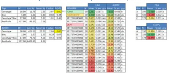
As described in Material and Methods, in addition to the AUDPC at 19dpi (end of the assay), studies were also made on the disease score attributed on the 7th day post inoculation because a very good discrimination was noticeable (from a score of 0.267 attributed to the resistant control to a score of 0.850 attributed to the most diseased plant). (Table 2)
Variance analysis postulates were verified (homoscedasticity, normality and independency (Annex IV). Thanks to this analysis, it was possible to observe that there are no block effects. This allowed us to treat all data together. It was possible to observe a significant effect related to the genotypes. This meant that each genotype did not react the same way to Aphanomyces cochlioides (Table 2).
b. Individuals distribution
A continuous distribution of the individual 7dpi scores and AUDPC can be observed. This showed a quantitative reaction of the genotype. The response did not follow a normal distribution (figure 20), but no standard transformation (log, ln, ln x+1, !) succeeded in normalizing it.
It is possible to see that FC607 is the most resistant (7dpi = 0.267 and AUDPC = 9.03), followed by the hybrid FC607*DKPP.DKPP, which is the susceptible line, which has a quite high AUDPC (12.05) and a moderately high 7dpi score (0.643), but some of the genotypes were already more susceptible (for example S11T27015S001 with a 7dpi score of 0.85 and an AUDPC of 12.82).
The fact that FC607’s AUDPC was not zero confirmed that it is responsible for a partial resistance because even the “resistant” genotype is contaminated.
c. Mean comparison
The Duncan test allowed the splitting of the accessions into groups (Table 2). On this table, it can be seen that only FC607 is really different from the other genotypes. This is confirmed by the same analysis made without the controls (Table 3). The Dunnett test (Table 4) shows a comparison between each genotype and the controls. In this assay, one can see that all genotypes (except the resistant and hybrid controls) are not significantly different from the susceptible control (p>0.05).
d. Heritability
Heritability (h2) is quite high for the two tested values (7dpi score and AUDPC). For AUDPC, h2=0.65 and for 7dpi, h2=0.75. Both measures are very close. This value shows that the phenotypic variation due to genetic differences is quite high.
2. Genetic analysis
a. Comparison of the three types of genotypes
As explained in Materials and Methods, three types of genotype are expected, demonstrating resistant, intermediate and susceptible phenotypes. However this is not the case. Indeed, one of the genotypes that theoretically should be one of the most susceptible appeared to be the most resistant (S11T27010S001). Moreover, ANOVA did not show any significant difference between the groups (p>0.05) (Table 5).
Table 6 : Kruskal-Wallis results with sampled individuals for experiment 1
Figure 21 : individuals repartition according to 7dpi’s score and AUDPC for experiment 2 Table 7 : 7dpi and AUDPC results for experiment 2: ANOVA, Duncan test
!" # $% & '& () *&
Table 8 : 7dpi and AUDPC results without controls for experiment
18
b. Kruskal-Wallis test
First, a Kruskal Wallis test was made on parental genotypes (chromosomes 4 and 6) with the mean of 7dpi score and AUDPC of each family. For both scores, no QTL were detectable.
The Kruskal-Wallis test performed with sampled individuals (for which leaves were sampled) clearly showed a significant effect of markers on chromosome 4, indeed, all markers on this chromosome had a significant K-value. By contrast, nothing was detected on chromosome 6. (Table 6)
D. Experiment 2
1. Statistical analysis
a. Analysis of variance
7dpi was also chosen in addition to AUDPC at 15dpi (end of the assay), because of a good discrimination (from a score of 0.3 attributed to the resistant control to a score of 0.933 attributed to the most diseased plant). (Table 7)
Homoscedasticity (equality of variance), normality and independence were verified for the variance analysis (Annex IV). Here again, one sees that there is no block effect and data can be treated together. And as with previous assay, it is possible to see a significant effect of the genotype.
b. Distribution of Individuals
Again, a continuous distribution of 7dpi score and AUDPC is observed, this is consistent with the fact that the resistance is quantitative. The distribution is not normal, but no transformation was found to correct it. (Figure 21)
c. Mean comparison
The Duncan test shows that the experiment worked well because the three controls are clearly discriminated.
With the groups formed by the Duncan test, only genotypes S13T30129S001 and S13T30094S001 are significantly different from the susceptible control DKPP (p<0.05) (Table 7). This is confirmed by the analysis without controls (Table 8). The Dunnett test (Table 9) shows that no genotypes are comparable to the resistant control, but with the 7dpi score, two genotypes (the two cited above) are significantly less infected than the susceptible control. With the AUDPC, besides those two, the genotype S13T30126S001 is also significantly less contaminated than the susceptible control, but again, they are significantly different from the resistant control.
d. Heritability
As in the previous assay, heritability is rather high for the 7dpi score and AUDPC. For AUDPC, h2=0.73 and for 7dpi, h2=0.66. They are also in the same range as the heritability values calculated in the forgoing assay.
2. Genetic analysis
a. Families result comparison
On table 10, it is possible to see that families with the highest number of individuals that seem to be more resistant (having a lot of A individuals, such as S13T30094S001, S13T30129S001 or S13T30126S001) are also generally more resistant (considering 7dpi
Table 10 : comparison of families results to genotypes for experiment 2
Table 11 : Kruskal-Wallis results for experiment 2
Figure 22 : Interval mapping results for experiment 2 with families values and parental genotype
Figure 23 : Interval mapping results for experiment 2 with sampled individuals
Table 12 : Means in regard to genotype for marker F107_S01
!"#$%& '()*&
19 score and AUDPC). It is noticeable that they have in general more markers with genotype coming from FC607, especially on chromosome 1.
b. Kruskal-Wallis test
This test allows the detection of significant effects. For the 7dpi score, a QTL is detected on chromosome 1 between markers A046_S02 and A062_S01, on chromosome 4 between markers D156_S01 and D075_S01 and D201_S01 and D093_S02. For the AUDPC, on chromosome 1, a QTL is detected between markers A046_S02 and A062_S01, on chromosome 4 a QTL is detected between markers D201_S01 and D093_S02. (Table 11)
For both 7dpi score and AUDPC, nothing is detectable on chromosome 6.
As it was explained in the Bibliography, this test gives just a preview of our data and is not the most reliable.
c. Interval mapping
First, we made the study on families, with the use of the parental genotype.
The significant threshold of the LOD was calculated by a permutation test with 1000 iterations. The result was a LOD score of 2.8 for the AUDPC and 3 for 7dpi score. These LOD score looks coherent (a usual value is situated around 3).
Interval mapping, which is more powerful than the previous Kruskal-Wallis test, showed only one significant QTL on chromosome 1 with a LOD score of 4.42 at 53 cM. This QTL is significant between 36 and 58 cM and has A046_S02 and A068_S01 as flanking markers. It is only significant for the 7dpi score. This QTL explains 71% of the phenotypic variance. (Figure 22)
For the AUDPC, a peak is detectable on chromosome 1 but it is not significant.
Then the analysis was made on all sampled individuals (individuals for which leaves were sampled). Only chromosomes 4 and 6 were genotyped.
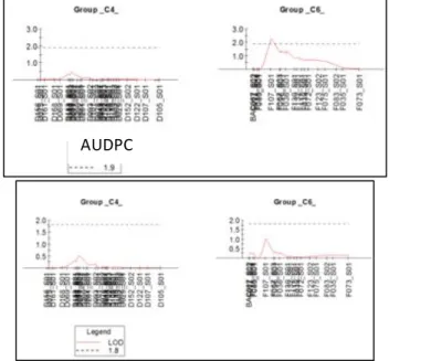
The LOD score is 1.8 for 7 dpi and 1.9 for AUDPC
Here, there is a significant QTL on chromosome 6. The highest LOD value is 2.28 at the marker F107_S01, for AUDPC (a peak is visible for 7dpi but it is not significant) (Figure 20) (Figure 23). With a further analysis (Table 12) allele B seems to gives the resistance. This confirms the analysis with families, saying that FC607 does not give a resistance QTL on chromosome 6.
d. Multiple QTL mapping
As is visible in figure 20, the QTL detected on chromosome 1 is not very precisely located. To improve the precision of the location, marker A062_S01 (50 cM) was put as cofactor, because it was the closest marker to the position of the QTL with interval mapping (Figure 24). Now, the QTL is significant between 50 and 58 cM with the maximum at 52 cM. This QTL explains 72% of the phenotypic variance. Individuals that carry the allele from FC607 (A) are more resistant than those with the allele from DKPP (B) (Table 13).
Figure 24 : Multiple QTL mapping for experiment 2 with A062_S01 as cofactor
Table 13 : Means in regard to genotype for marker A025_S02