Three Hot-Jupiters on the upper edge of the mass-radius
distribution: WASP-177, WASP-181 and WASP-183
Oliver D. Turner,
1
?
D.R. Anderson,
2
K. Barkaoui,
3,4
, F. Bouchy,
1
Z. Benkhaldoun
4
D.J.A. Brown,
5,6
A. Burdanov,
3
A. Collier Cameron,
7
E. Ducrot,
3
M. Gillon,
3
C. Hellier,
2
E. Jehin,
3
M. Lendl,
8,1
P.F.L. Maxted,
2
L.D. Nielsen,
1
F. Pepe,
1
D. Pollacco,
5,6
F.J. Pozuelos,
3
D. Queloz,
1,9
D. S´
egransan,
1
B. Smalley,
2
A.H.M.J. Triaud,
10
S. Udry
1
, and R.G. West
5,6
1Observatoire de Gen`eve, Universit´e de Gen`eve, 51 Chemin des Maillettes, 1290 Sauverny, Switzerland 2Astrophysics Group, Keele University, Staffordshire ST5 5BG, UK
3Space sciences, Technologies and Astrophysics Research (STAR) Institute, Universit´e de Li`ege, Li`ege 1, Belgium
4Oukaimeden Observatory, High Energy Physics and Astrophysics Laboratory, Cadi Ayyad University, Marrakech, Morocco 5Department of Physics, University of Warwick, Coventry CV4 7AL, UK
6Centre for Exoplanets and Habitability, University of Warwick, Gibbet Hill Road, Coventry CV4 7AL, UK 7SUPA, School of Physics and Astronomy, University of St. Andrews, North Haugh, Fife KY16 9SS, UK 8Space Research Institute, Austrian Academy of Sciences, Schmiedlstr. 6, A-8042 Graz, Austria
9Cavendish Laboratory, J J Thomson Avenue, Cambridge CB3 0HE, UK
10School of Physics & Astronomy, University of Birmingham, Edgbaston, Birmingham, B15 2TT, UK
Accepted XXX. Received YYY; in original form ZZZ
ABSTRACT
We present the discovery of 3 transiting planets from the WASP survey, two hot-Jupiters: WASP-177 b (∼0.5 MJup, ∼1.6 RJup) in a 3.07-d orbit of a V = 12.6 K2 star, WASP-183 b (∼0.5 MJup, ∼1.5 RJup) in a 4.11-d orbit of a V = 12.8 G9/K0 star;
and one hot-Saturn planet WASP-181 b (∼0.3 MJup, ∼1.2 RJup) in a 4.52-d orbit of a
V = 12.9 G2 star. Each planet is close to the upper bound of mass-radius space and has a scaled semi-major axis, a/R∗, between 9.6 and 12.1. These lie in the transition
between systems that tend to be in orbits that are well aligned with their host-star’s spin and those that show a higher dispersion.
Key words: planets and satellites: detection – planets and satellites: individual: WASP-177b – planets and satellites: individual: WASP-181b – planets and satellites: individual: WASP-183b
1 INTRODUCTION
Since the beginning of the project the Wide Angle Search for Planets (WASP; Pollacco et al. 2006) survey has dis-covered nearly 190 transiting, close-in, giant exoplanets. As they transit their host stars their bulk properties, mass and radius, can be determined relatively easily. Their transits al-low for deeper characterisation that has led to the discovery of multiple chemical and molecular species in their atmo-spheres (Birkby et al. 2013;de Kok et al. 2013;Wyttenbach et al. 2017;Hoeijmakers et al. 2018) and the observation of planetary winds (Brogi et al. 2016).
Close-in exoplanets can also provide information on the
? E-mail: [email protected]
formation and migration mechanisms of solar systems. It is expected that hot-Jupiter exoplanets initially form much further from their stars than where we detect them today. Therefore some mechanism must cause this migration. There are two proposed pathways, high eccentricity migration or disk migration. In the former some mechanism e.g. Kozai cy-cles (Wu & Murray 2003;Armitage 2013) or planet-planet scattering (Rasio & Ford 1996; Weidenschilling & Marzari 1996), forces the cold Jupiter into a highly eccentric orbit which then is tidally circularised via interaction with the star. During this kind of migration it is possible for the planet orbital axis to become mis-aligned with the stellar spin axis (Fabrycky & Tremaine 2007). In the latter mech-anism the planet loses angular momentum via interaction with the stellar disk during formation and migrates inward
(Goldreich & Tremaine 1980). This is expected to preserve the initial spin-orbit alignment (Marzari & Nelson 2009), though work is being done to investigate the production of mis-aligned planets due to inclined protoplanetary discs (Xiang-Gruess & Kroupa 2017).
The alignment between the stellar rotation axis and planet orbit can be investigated with the Rossiter-McLaughlin (RM) technique (Rossiter 1924; McLaughlin 1924; Triaud et al. 2010, etc.). These observations have shown a general trend for systems orbiting cool stars (with Teff < 6250K;Albrecht et al. 2012;Anderson et al. 2015b) to be more well aligned than systems orbiting hotter stars. Tides are also expected to play a role. In cool star systems, those with smaller scaled semi-major axes, a/R∗, tend to be more often well aligned than those with larger a/R∗. Though this picture is far from clear as there seems to be evidence for the hot/cool alignment disparity holding even for sys-tems with large separations or low mass planets meaning tidal effects should be minimal (Mazeh et al. 2015) casting tidal realignment into doubt (see also the discussion ofDai & Winn 2017).
In this paper we present the discovery of three systems at the upper edge of the mass-radius envelop of hot-giants that could be useful probes of tidal re-alignment.
2 OBSERVATIONS
Each of these planets was initially flagged as a candidate in data taken with both WASP arrays located at Roque de los Muchachos Observatory on La Palma and at the South African Astronomical Observatory (SAAO). The data were searched for periodic signals using a BLS method as per
Collier Cameron et al.(2006,2007). The survey itself is de-scribed in more detail byPollacco et al.(2006).
In order to confirm the planetary nature of the signals radial velocity (RV) data were obtained with the CORALIE spectrograph on the 1.2-m Swiss telescope at La Silla, Chile (Queloz et al. 2000). Additional photometry was acquired using EulerCam (Lendl et al. 2012, also on the 1.2-m Swiss) and the two 0.6-m TRAPPIST telescopes (Gillon et al. 2011;
Jehin et al. 2011), based at La Silla and Oukaimeden Obser-vatory in Morocco (Gillon et al. 2017;Barkaoui et al. 2018). Due to the low masses of WASP-181 b and WASP-183 b, we also acquired HARPS data1. These observations are sum-marised in Table1. The TRAPPIST data from 2018-08-13 contain a meridian flip at BJD = 2458344.5639. During anal-ysis the data were partitioned at this point and modeled as two datasets.
Figures ??,1and2show the phase folded discovery and follow-up data. The RVs exhibit signals in phase with those found in the transit data and are consistent with compan-ion objects of planetary mass. We checked for correlatcompan-ion between the RV variation and the bisector spans, see Fig.3. We find no strong correlation and so further exclude the possibility that these objects are transit mimics.
1 These observations were made as part of the programs Anderson:0100.C-0847(A) and Nielsen:0102.C-0414(A).
Relative flux 0.96 0.98 1 1.02 0.4 0.6 0.8 1 1.2 1.4 1.6 Relative flux WASP TRAP. I+z 2016-12-06 Trap I+z 2017-07-29 Euler I 2017-09-03 0.88 0.89 0.9 0.91 0.92 0.93 0.94 0.95 0.96 0.97 0.98 0.99 1 1.01 1.02 1.03 0.96 0.98 1 1.02 1.04
Relative radial velocity / m s
-1 Orbital phase -100 0 100 0.4 0.6 0.8 1 1.2 1.4 1.6
Figure 1. As for Fig.?? for the WASP-181 system. CORALIE data in bottom figure are small (red) while HARPS data are larger (blue) symbols.
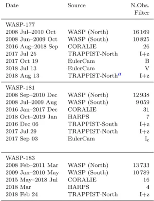
Table 1. Observations of WASP-177, WASP-181 and WASP-183.
Date Source N.Obs.
Filter WASP-177
2008 Jul–2010 Oct WASP (North) 16 169 2008 Jun–2009 Oct WASP (South) 10 825
2016 Aug–2018 Sep CORALIE 26
2017 Jul 25 TRAPPIST-North I+z
2017 Oct 19 EulerCam B
2018 Jul 13 EulerCam V
2018 Aug 13 TRAPPIST-Northa I+z WASP-181
2008 Sep–2010 Dec WASP (North) 12 938 2008 Jul–2009 Aug WASP (South) 9 059
2016 Jan–2017 Dec CORALIE 31
2018 Oct–2019 Jan HARPS 7
2016 Dec 06 TRAPPIST-South I+z
2017 Jul 29 TRAPPIST-North I+z
2017 Sep 03 EulerCam Ic
WASP-183
2008 Feb–2011 Mar WASP (North) 13 733 2009 Jan–2010 May WASP (South) 10 789
2015 May–2018 Jul CORALIE 16
2018 Mar HARPS 4
2018 Feb 24 TRAPPIST-North I+z
a Meridian flip at BJD 2458344.5639.
3 ANALYSIS
3.1 Stellar Parameters
To obtain the stellar parameters effective temperature, Teff, metallicity, [Fe/H], and surface gravity, log g, we followed the method of Giles et al. (2018a,b) using iSpec ( Blanco-Cuaresma et al. 2014b). To do this we corrected each spec-trum for the computed RV shift, cleaned them of cosmic ray strikes and convolved them to a spectral resolution, R, of47 000. Then, ignoring areas typically affected by tel-luric lines we used the synthetic spectral fitting technique to derive the stellar parameters. Via iSpec we used SPEC-TRUM (Gray & Corbally 1994) as the radiative transfer code with atomic data from VALD (Kupka et al. 2011), a line selection based on a R ∼ 47 000 solar spectrum ( Blanco-Cuaresma et al. 2016,2017) and the MARCS model atmo-spheresGustafsson et al.(2008) in the wavelength range 480-to 680-nm. We increased the uncertainties in these param-eters by adding the dispersion found by analysing the Gaia benchmark stars with iSpec as per Blanco-Cuaresma et al.
(2014a);Jofr´e et al.(2014);Heiter et al.(2015).
We determined the stellar density from and initial fit to the lightcurves and then used it along with the Teff and metallicity to determine stellar masses, for later use in the joint analysis, and the stellar ages with the Bayesian stel-lar evolution code BAGEMASS (Maxted et al. 2015). The resulting parameters are presented in the top part of Ta-ble 3and the corresponding isochrons/evolutionary tracks are shown in Fig4.
BAGEMASS uses an MCMC with a densely sampled
grid of stellar models to compute stellar masses and ages. There are three usable grids with differing mixing length pa-rameters,αMLT, and helium enhancement. The default val-ues of these areαMLT = 1.78 and no He-enhancement. We used the BAGEMASS default parameters to model 177 and 181 but found that they did not fit WASP-183 very well. This is likely because WASP-WASP-183 is among the ∼ 3% of the K-dwarf population that are larger than mod-els would predict (Spada et al. 2013). To account for this we follow the method ofMaxted et al.(2015) in the case of Qatar-2 and use a the grid provided by BAGEMASS with αMLT = 1.5. This results in a much improved fit to the ob-served density and temperature. We find that the resulting mass estimate is unaffected.
3.2 System parameters
To determine the system parameters we modeled the dis-covery and follow-up data together using the most recent version of the Markov-Chain Monte Carlo (MCMC) code described in detail inCollier Cameron et al.(2007) and An-derson et al. (2015a). We modeled the transit lightcurves using the models of Mandel & Agol(2002) with the 4 pa-rameter limb darkening law ofClaret(2000,2004).
In brief, the models were initialised using the period, P, epoch, T0, transit depth, (Rp/Rs)2, transit duration, T14, and impact parameter, b, output by the BLS search of each discovery lightcurve. The spectroscopic stellar effective tem-perature, Teff, and metallicity, [Fe/H], were used initially to estimate the stellar mass using the updated Torres mass cal-ibration bySouthworth(2011). To explore the effect of limb-darkening we extracted tables of limb- limb-darkening parameters in each photometric band used for each star. They were ex-tracted for a range of effective temperatures while keeping the stellar metallicity and surface gravity constant. The val-ues used were perturbed during the MCMC via TL−D, the ‘limb-darkening temperature’, which has a mean and stan-dard deviation corresponding to the spectroscopic Teff and its uncertainty.
At each step of the MCMC each of these values are perturbed and the models are re-fit. These new proposed parameters are then accepted if the χ2of the fit is better or accepted with a probability proportional to exp(−∆ χ2) if the χ2 of the fit is worse.
In the final MCMCs, in place of using the Torres rela-tion to determine a mass, we provided the value given by BAGEMASS. The code then drew values at each step from a Gaussian with a mean and standard deviation given by the value and its uncertainty respectively. Due to the lack of good quality follow-up photometry we imposed a similar prior on the radius of the star WASP-183 using the Gaia par-allax. Lacking a complete, good quality follow-up lightcurve can lead to a poor determination of, ∆F, T14and b which we use to calculate the R∗/a. This in turn results in a poorer determination of R∗, Rp and other parameters that depend upon them.
In this way we also explored models allowing for ec-centric orbits and the potential for linear drifts in the RVs. There was no strong evidence supporting either scenario so we present the system solutions corresponding to circular orbits (Anderson et al. 2012) with no trends due to unseen
Table 2. Periodogram analysis for WASP lightcurves of WASP-177.
WASP Dates Period Amp FAP Notes
Inst. JD-2450000 Prot(d) (mag.)
North 4656-4767 7.569 0.005 0.0017 P/2 North 5026-5131 7.528 0.006 <0.0001 P/2 North 5387-5498 14.860 0.004 <0.0001 South 4622-4764 14.330 0.005 0.0007 South 4984-5129 7.456 0.006 <0.0001 P/2
companions. The parameters derived by these fits can be found in the lower part of Table3.
3.3 Rotational modulation
We checked the WASP lightcurves of the three stars for ro-tational modulation that could be caused by star spots using the method described byMaxted et al.(2011). The transits were fit with a simple model and removed. We performed the search over 16384 frequencies ranging from 0 to 1 cycles/day. Due to the limited lifetime and variable distribution of star spots this modulation is not expected to be coherent over long periods of time. As such, we modeled each season of data from each camera individually. 181 and WASP-183 show no significant modulation, with an upper limit on the amplitude of 2- and 3-mmag respectively.
However, WASP-177 was found to exhibit modulation consistent with a rotational period, Prot = 14.86 ± 0.14 days and amplitude of 5 ± 1 mmag. The results of this analysis for each camera and season of data is shown in Table 2. Fig. 5 shows the periodograms of the fits and the discov-ery lightcurves phase-folded on the corresponding period of modulation. Three of the datasets exhibit Prot∼ 7-days while the other two exhibit Prot ∼ 14-days. We interpret the ∼ 7-day signals as a harmonic of the longer ∼ 14-7-day signal as it is more easy for multiple active regions to produce a ∼ 7-day signal when the true period is ∼ 14-days than vice versa. Us-ing this rotational period and our value for the stellar radius we find a stellar rotational velocity of, v∗ = 2.9 ± 0.2 km/s. When compared to the projected equatorial spin velocity we find a stellar inclination to our line of sight of 38 ± 25◦which suggests that WASP-177 b could be quite mis-aligned.
4 DISCUSSION
Our joint analysis shows that in this ensemble we have two large sub-Jupiter mass planets: WASP-177 b (∼0.5 MJup, ∼1.6 RJup) and WASP-183 b (∼0.5 MJup, ∼1.5 RJup) orbit-ing old stars. The third planet, WASP-181 b, is a large Sat-urn mass planet (∼0.3 MJup, ∼1.2 RJup) . According to the analysis with BAGEMASS, WASP-177 and WASP-183 are both at the latter end of the main sequence explaining their slightly larger radii for stars of their spectral class; a 9.7±3.9 Gyr K2 and 14.9 ± 1.7 Gyr G9/K0 respectively. WASP-183 is particularly noteworthy as its advanced age makes it one of the oldest stars known to host a transiting planet (see Fig.6). Though, WASP-183 appears to be subject to the K-dwarf radius anomaly, making this determination less clear.
Meanwhile, WASP-181 is a relatively young, standard ex-ample of a G2 star.
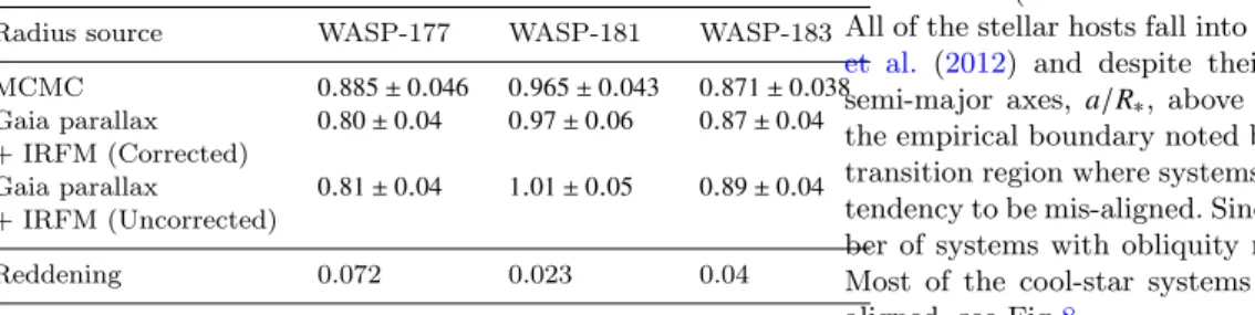
We compared the stellar radii derived from our MCMC to those we can calculate using the Gaia DR2 parallaxes (Luri et al. 2018;Gaia Collaboration et al. 2018), with the correction fromStassun & Torres(2018), and stellar angular radii from the infra-red flux fitting method (IRFM) these radii, with reddening accounted for by the use of dust maps (Schlafly & Finkbeiner 2011). We find good agreement and present a summary in table4.
All three planets occupy the upper edge of the mass-radius distribution, seen in Fig 7. WASP-181 b is amongst the group of the largest planets for an object of its mass. While its mass is not as well determined as the other two, further HARPS observations will help to refine this. WASP-177 b and WASP-183 b do lie above the bulk of the distribu-tion, especially when compared to other objects with mass determinations of 10% precision or better. However, it is difficult to say how exceptional they are as a precise radius determination has proven difficult for them both. The transit of WASP-177 b is grazing and the transit of WASP-183 b, in addition to being grazing, lacks a full high precision follow-up lightcurve to refine the transit shape. We anticipate that TESS observations could soon solve the latter problem;the long cadence data would capture roughly 24 in transit points with a predicted precision from the ticgen tool of better than 1000 ppm in each 30-minute observation.
We used the the values derived for planet equilibrium temperature, Teq, and surface gravity, g, along with Boltz-mann’s constant, k, and the atmospheric mean molecular mass, µ, to estimate the scale heights, H, of these planets as:
H= kTeq
gµ (1)
assuming an isothermal, hydrogen dominated atmo-sphere. The resulting scale heights were; 790 ± 320 km, 770±200 km, 696±464 km for WASP-177 b, WASP-181 b and WASP-183 b respectively. These translate to transit depth variations of just under 300 ppm for 177 and WASP-181 and ∼ 300 ppm for WASP-183. If we account for the K-band flux and scale in the same way asAnderson et al.
(2017), we get atmospheric signals of; 70, 41 and 60. In re-ality, we can expect this metric to be an over estimate of detectability for WASP-177 b and WASP-183 b as the graz-ing nature of their transits reduces the impact of the atmo-spheric signal further. For comparison we used the same met-ric on other planets with atmosphemet-ric detections: water has been detected in the atmospheres of both WASP-12 b ( Krei-dberg et al. 2015; signal ∼ 93) and WASP-43 b (Kreidberg et al. 2014; signal ∼ 74); titanium oxide has been detected in the atmosphere of WASP-19 b (Sedaghati et al. 2017; signal ∼ 83); sodium and potassium have both been detected in the atmosphere of WASP-103 b (Lendl et al. 2017; signal ∼ 37). While not ideal targets, this suggests such detections may be possible.
Investigation into any eccentricity or long-period mas-sive companions in these systems has not yielded anything convincing. All of the orbits are circular, with the 2σ upper limits quoted in Table3. As for long term trends, WASP-177 shows the possibility of a very low significance (∼ 1.5σ) drift
Table 3. System parameters
Parameter Symbol (Unit) WASP-177 WASP-181 WASP-183
1SWASP ID − J221911.19-015004.7 J014710.37+030759.0 J105509.36-004413.7
Right ascension (h:m:s) 22:19:11.19 01:47:10.37 10:55:09.36
Declination (◦:’:”) -01:50:04.7 +03:07:59.0 -00:44:13.7
V magnitude − 12.58 12.91 12.76
Spectral typea − K2 G2 G9/K0
Stellar effective temperature Teff (K) 5017 ± 70 5839 ± 70 5313 ± 72
Stellar surface gravity log(g) (cgs) 4.49 ± 0.07 4.38 ± 0.08 4.25 ± 0.09 Stellar metallicity [Fe/H] (dex) 0.25 ± 0.04 0.09 ± 0.04 −0.31 ± 0.04 Projected equatorial spin velocity V∗sin I∗ (km/s) 1.8 ± 1.0 3.3 ± 0.9 1.0 ± 1.0
Stellar macro-turbulent velocityb Vmac(km/s) 2.7 3.3 2.8
Stellar age (Gyr) 9.7 ± 3.9 2.5 ± 1.7 14.9 ± 1.7
Distancec (pc) 178 ± 2 443 ± 8 328 ± 4
Period P (d) 3.071722 ± 0.000001 4.5195064 ± 0.0000034 4.1117771 ± 0.0000051 Transit Epoch T0− 2450000 7994.37140 ± 0.00028 7747.66681 ± 0.00035 7796.1845 ± 0.0024 Transit Duration T14 (d) 0.0672 ± 0.0013 0.1277 ± 0.0015 0.084 ± 0.005 Scaled Semi-major Axis a/Rs 9.61+0.42−0.53 12.09 ± 0.54 11.44 ± 0.54
Transit Depth (Rp/Rs)2 0.0185+0.0035 −0.0014 0.01590 ± 0.00038 0.0226+0.0060−0.0036 Impact Parameter b 0.980+0.092−0.060 0.34+0.10−0.15 0.916+0.163−0.091 Orbital Inclination i (◦) 84.14+0.66−0.83 88.38+0.76−0.59 85.37+0.61−0.88 Systemic Velocity γ (kms−1) −7.1434 ± 0.0041 −8.5489 ± 0.0072 68.709 ± 0.012 Semi-amplitude K1(ms−1) 77.3 ± 5.2 35.7 ± 3.9 74.8 ± 6.6
Semi-major Axis a (au) 0.03957 ± 0.00058 0.05427 ± 0.00069 0.04632 ± 0.00075
Stellar Mass Ms(M ) 0.876 ± 0.038 1.04 ± 0.04 0.784 ± 0.038
Stellar Radius Rs(R ) 0.885 ± 0.046 0.965 ± 0.043 0.871 ± 0.038
Stellar Density ρs(ρ ) 1.26+0.23−0.15 1.16 ± 0.15 1.19 ± 0.17
Stellar Surface Gravity log(gs) (cgs) 4.486+0.049−0.037 4.487 ± 0.039 4.452 ± 0.043
Limb-darkening Temperature TL−D (K) 5012 ± 69 5835 ± 70 5313 ± 72
Stellar Metallicity [Fe/H] 0 ± 0 0 ± 0 0 ± 0
Planet Mass Mp (MJup) 0.508 ± 0.038 0.299 ± 0.034 0.502 ± 0.047
Planet Radius Rp (RJup) 1.58+0.66−0.36 1.184+0.071−0.059 1.47+0.94−0.33 Planet Density ρp (ρJup) 0.130+0.153−0.085 0.179 ± 0.033 0.16+0.18−0.12 Planet Surface log(gp) (cgs) 2.67+0.22−0.31 2.686 ± 0.065 2.72+0.22−0.43 Planet Equilibrium Temperatured Te q(K) 1142 ± 32 1186+32−26 1111 ± 30
a Spectral type estimated by comparison of Teffto the table inGray(2008). b Derived via the method ofDoyle et al.(2014).
c From Gaia DR2Gaia Collaboration et al.(2016,2018);Luri et al.(2018). d Assuming 0 albedo and complete redistribution of heat.
Table 4. Comparison of stellar radii output by the MCMC analysis with radii derived from Gaia DR2.
Radius source WASP-177 WASP-181 WASP-183 MCMC 0.885 ± 0.046 0.965 ± 0.043 0.871 ± 0.038 Gaia parallax 0.80 ± 0.04 0.97 ± 0.06 0.87 ± 0.04 + IRFM (Corrected) Gaia parallax 0.81 ± 0.04 1.01 ± 0.05 0.89 ± 0.04 + IRFM (Uncorrected) Reddening 0.072 0.023 0.04
with δγ/δt of (−2.4 ± 1.6) × 10−5 km/s/d. Neither WASP-181 nor WASP-183 show significant drifts with δγ/δt of (1.2 ± 4.0) × 10−5 km/s/d and (−1.9 ± 5.1) × 10−5 km/s/d respectively.
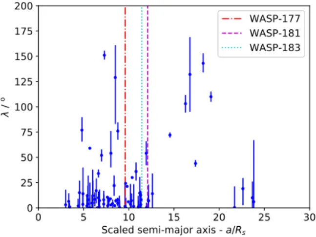
Finally, these systems do present interesting targets for the investigation of the observed spin-orbit mis-alignment distribution (Albrecht et al. 2012;Anderson et al. 2015b). All of the stellar hosts fall into the ”cool” regime ofAlbrecht et al. (2012) and despite their short periods have scaled semi-major axes, a/R∗, above 8. They are therefore above the empirical boundary noted byDai & Winn(2017) as the transition region where systems with cooler stars show more tendency to be mis-aligned. Since the study in 2017 the num-ber of systems with obliquity measurements has increased. Most of the cool-star systems with a/R∗ above 8 are well aligned, see Fig8.
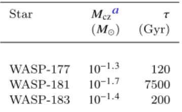
We estimated the alignment time-scale for each system using Eq.4 ofAlbrecht et al.(2012) as was done for WASP-117 (Lendl et al. 2014). These time-scales, along with the mass of the convective zone, Mcz, are shown in Tab5. In each case, the time-scale for realignment is much longer than the
Table 5. Convective zone masses and estimated time-scales for realignment of systems in this paper.
Star Mcza τ
(M ) (Gyr)
WASP-177 10−1.3 120 WASP-181 10−1.7 7500 WASP-183 10−1.4 200
a Dervied fromPinsonneault et al.(2001).
ages of the systems. Therefore, we would expect the initial state of alignment of the systems to have been preserved. We have estimated the inclination of WASP-177 to be 38 ± 25◦ and so may expect it to join only 12 systems with a/R∗ < 15 that show mis-alignment this makes it a potentially important diagnostic in determining the factors that cause or preserve mis-alignment.
We calculate that the amplitude of the RM effect will be greatest for WASP-181 at ∼ 50 ms−1. The effect should also be detectable for WASP-177 and WASP-183 despite their more grazing transits, with an amplitude of ∼ 10 ms−1.
5 CONCLUSIONS
We have presented the discovery of 3 transiting exoplanets from the WASP survey; WASP-177 b (∼0.5 MJup, ∼1.6 RJup), WASP-181 b (∼0.3 MJup, ∼1.2 RJup), and WASP-183 b (∼0.5 MJup, ∼1.5 RJup). They all occupy the upper region of the mass-radius distribution for hot gas-giant planets but do not present exceptional targets for transmission spectroscopy. However, regarding the investigation of system spin-orbit alignment they do occupy an under investigated range of a/R∗ and so could act as good probes of tidal realignment time-scales.
ACKNOWLEDGEMENTS
We thank the Swiss National Science Foundation (SNSF) and the Geneva University for their continuous support to our planet search programs. This work has been in particu-lar carried out in the frame of the National Centre for Com-petence in Research ‘PlanetS’ supported by the Swiss Na-tional Science Foundation (SNSF). WASP-South is hosted by the South African Astronomical Observatory and we are grateful for their ongoing support and assistance. Funding for WASP comes from consortium universities and from the UK’s Science and Technology Facilities Council. TRAP-PIST is funded by the Belgian Fund for Scientific Research (Fond National de la Recherche Scientifique, FNRS) under the grant FRFC 2.5.594.09.F, with the participation of the Swiss National Science Fundation (SNF). MG is a F.R.S.-FNRS Senior Research Associate. The research leading to these results has received funding from the European Re-search Council under the FP/2007-2013 ERC Grant Agree-ment 336480, from the ARC grant for Concerted Research Actions financed by the Wallonia-Brussels Federation, from
the Balzan Foundation, and a grant from the Erasmus+ In-ternational Credit Mobility programme (K Barkaoui). We thank our anonymous reviewer for their comments which helped improve the clarity of the paper.
REFERENCES
Albrecht S., et al., 2012,ApJ,757, 18
Anderson D. R., et al., 2012,MNRAS,422, 1988 Anderson D. R., et al., 2015a,A&A,575, A61 Anderson D. R., et al., 2015b,ApJ,800, L9 Anderson D. R., et al., 2017,A&A,604, A110
Armitage P. J., 2013, Astrophysics of Planet Formation. Cam-bridge University Press
Barkaoui K., et al., 2018, preprint, (arXiv:1807.06548) Birkby J. L., de Kok R. J., Brogi M., de Mooij E. J. W., Schwarz
H., Albrecht S., Snellen I. A. G., 2013,MNRAS,436, L35 Blanco-Cuaresma S., Soubiran C., Jofr´e P., Heiter U., 2014a,
A&A,566, A98
Blanco-Cuaresma S., Soubiran C., Heiter U., Jofr´e P., 2014b, A&A,569, A111
Blanco-Cuaresma S., et al., 2016, in 19th Cambridge Workshop on Cool Stars, Stellar Systems, and the Sun (CS19). p. 22, doi:10.5281/zenodo.155115
Blanco-Cuaresma S., et al., 2017, in Highlights on Spanish Astro-physics IX. pp 334–337
Brogi M., de Kok R. J., Albrecht S., Snellen I. A. G., Birkby J. L., Schwarz H., 2016,ApJ,817, 106
Claret A., 2000, A&A,363, 1081 Claret A., 2004,A&A,428, 1001
Collier Cameron A., et al., 2006,MNRAS,373, 799 Collier Cameron A., et al., 2007,MNRAS,380, 1230 Dai F., Winn J. N., 2017,AJ,153, 205
Doyle A. P., Davies G. R., Smalley B., Chaplin W. J., Elsworth Y., 2014,MNRAS,444, 3592
Fabrycky D., Tremaine S., 2007,ApJ,669, 1298 Gaia Collaboration et al., 2016,A&A,595, A1 Gaia Collaboration et al., 2018,A&A,616, A1 Giles H. A. C., et al., 2018a,MNRAS,475, 1809 Giles H. A. C., et al., 2018b,A&A,615, L13 Gillon M., et al., 2011,A&A,533, A88 Gillon M., et al., 2017,Nature,542, 456 Goldreich P., Tremaine S., 1980,ApJ,241, 425
Gray D. F., 2008, The Observation and Analysis of Stellar Pho-tospheres. Cambridge University Press
Gray R. O., Corbally C. J., 1994,AJ,107, 742
Gustafsson B., Edvardsson B., Eriksson K., Jørgensen U. G., Nordlund ˚A., Plez B., 2008,A&A,486, 951
Heiter U., Jofr´e P., Gustafsson B., Korn A. J., Soubiran C., Th´evenin F., 2015,A&A,582, A49
Hoeijmakers H. J., et al., 2018,Nature,560, 453 Jehin E., et al., 2011, The Messenger,145, 2 Jofr´e P., et al., 2014,A&A,564, A133 Kreidberg L., et al., 2014,ApJ,793, L27 Kreidberg L., et al., 2015,ApJ,814, 66
Kupka F., Dubernet M. L., VAMDC Collaboration 2011,Baltic Astronomy,20, 503
Lendl M., et al., 2012,A&A,544, A72 Lendl M., et al., 2014,A&A,568, A81
Lendl M., Cubillos P. E., Hagelberg J., M¨uller A., Juvan I., Fossati L., 2017,A&A,606, A18
Luri X., et al., 2018,A&A,616, A9 Mandel K., Agol E., 2002,ApJ,580, L171 Marzari F., Nelson A. F., 2009,ApJ,705, 1575 Maxted P. F. L., et al., 2011,PASP,123, 547
Maxted P. F. L., Serenelli A. M., Southworth J., 2015,A&A,575, A36
Mazeh T., Perets H. B., McQuillan A., Goldstein E. S., 2015, ApJ,801, 3
McLaughlin D. B., 1924,ApJ,60
Pinsonneault M. H., DePoy D. L., Coffee M., 2001,ApJ,556, L59 Pollacco D. L., et al., 2006,PASP,118, 1407
Queloz D., et al., 2000, A&A,354, 99
Rasio F. A., Ford E. B., 1996,Science,274, 954 Rossiter R. A., 1924,ApJ,60
Schlafly E. F., Finkbeiner D. P., 2011,ApJ,737, 103 Sedaghati E., et al., 2017,Nature,549, 238
Southworth J., 2011,MNRAS,417, 2166
Spada F., Demarque P., Kim Y. C., Sills A., 2013,ApJ,776, 87 Stassun K. G., Torres G., 2018,ApJ,862, 61
Triaud A. H. M. J., et al., 2010,A&A,524, A25 Weidenschilling S. J., Marzari F., 1996,Nature,384, 619 Wu Y., Murray N., 2003,ApJ,589, 605
Wyttenbach A., et al., 2017,A&A,602, A36
Xiang-Gruess M., Kroupa P., 2017,MNRAS,471, 2334
de Kok R. J., Brogi M., Snellen I. A. G., Birkby J., Albrecht S., de Mooij E. J. W., 2013,A&A,554, A82
Relative flux 0.96 0.98 1 1.02 1.04 0.4 0.6 0.8 1 1.2 1.4 1.6 Relative flux WASP TRAP. I+z 2018-02-24 0.93 0.94 0.95 0.96 0.97 0.98 0.99 1 1.01 1.02 1.03 0.96 0.98 1 1.02 1.04
Relative radial velocity / m s
-1 Orbital phase -200 -100 0 100 0.4 0.6 0.8 1 1.2 1.4 1.6
−400 −300 −200 −100 0 100 200 −400 −300 −200 −100 0 100 200 300 Bisector span / m s −1
Relative radial velocity / m s−1 WASP−177 7600 7700 7800 7900 8000 8100 8200 8300 8400 JD − 2450000 −300 −200 −100 0 100 200 300 −200 −100 0 100 200 Bisector span / m s −1
Relative radial velocity / m s−1 WASP−181 7600 7700 7800 7900 8000 8100 8200 8300 8400 JD − 2450000 −300 −200 −100 0 100 200 300 −200 −150 −100 −50 0 50 100 150 200 Bisector span / m s −1
Relative radial velocity / m s−1 WASP−183 7600 7700 7800 7900 8000 8100 8200 8300 8400 JD − 2450000
Figure 3. Radial velocity measurements plotted against line bi-sector spans. There is no strong correlation between the two, thus ruling out transit mimics. Solid lines are the linear best fit to the data. The dotted lines show the 1σ uncertainty limits on the fit.
4000 4500 5000 5500 6000 6500 Teff / K 0.0 0.5 1.0 1.5 2.0 2.5 ρs / ρ⊙ WASP-17713.9 Gyr 0.85 M⊙ WASP-181 0.84 Gyr 1.07 M⊙ WASP-183 17.2 Gyr 0.77 M⊙
Figure 4. Isochrones (solid/blue) and evolution tracks (dot-dashed/red) output by BAGEMASS for each of the planets we present with the corresponding isochrone age and mass (labelled).
Figure 5. Left: Periodograms of the WASP lightcurves of WASP-177. Each is labeled with the corresponding camera ID, dates of the observation period (in JD-2450000) and period of the most significant signal. Horizontal lines indicate false-alarm probability levels of 0.1, 0.01 and 0.001. Right: Lightcurves folded on the most significant detected period.
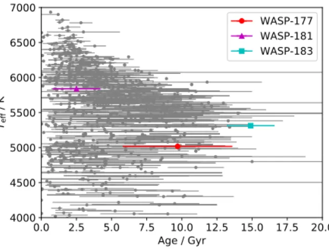
0.0 2.5 5.0 7.5 10.0 12.5 15.0 17.5 20.0 Age / Gyr 4000 4500 5000 5500 6000 6500 7000 Teff / K WASP-177 WASP-181 WASP-183
Figure 6. Age distribution for known exoplanet hosts with pub-lished uncertainties (grey) and planets presented in this paper (see legend). WASP-183 appears to be particularly old amongst planet hosts. However, we note it is unphysically old and so cau-tion that this determinacau-tion may be in part due to the K-dwarf radius anomaly. (Data from exoplanet.eu.)
10−1 100
Planet Mass /MJup
0.50 0.75 1.00 1.25 1.50 1.75 2.00 2.25 2.50 Pl an et R ad iu s /RJu p WASP-177 WASP-181 WASP-183
Figure 7. Mass-radius distribution for transiting planets. planets with masses determined to better than 10% precision are plotted in blue, otherwise the symbols are gray. 177 b, WASP-181 b and WASP-183 b have been plotted with their error bars. Each is close to the upper most part of the distribution. WASP-177 b is in an area particularly sparsely populated by planets with well determined masses. (Prepared using data collated the TEP-Cat.)
0
5
10
15
20
25
30
Scaled semi-major axis -
a/
Rs0
25
50
75
100
125
150
175
200
λ/
oWASP-177
WASP-181
WASP-183
Figure 8. Distribution of planets with measured spin-orbit an-gles with cool host stars. WASP-177, WASP-181 and WASP-183 are all cool stars by this definition and the planets lie in the re-gion where mis-alignment is often said to become more common. WASP-177 shows signs of being misaligned and so may be an interesting diagnostic in this region.
Table A1. Data from WASP
BJD -2450000 Diff. Mag. Target
magnitude error 5026.54902768 -0.00254900 0.01949100 WASP-177 5026.54946749 0.02243000 0.01957700 WASP-177 5026.55550916 -0.00315500 0.01926500 WASP-177 5026.55596055 -0.00210900 0.01891800 WASP-177 5026.56091425 0.02301800 0.01892700 WASP-177 5026.56135407 -0.01070600 0.01829000 WASP-177 5026.56629620 -0.01820900 0.01836500 WASP-177 5026.56673601 -0.03087100 0.01769000 WASP-177 5026.57268508 -0.02453400 0.01780000 WASP-177 5026.57312490 -0.00700800 0.01818600 WASP-177
Table A2. Data from Trappist
BJD -2450000 Dif. Mag. Mag. error Filter Target
7960.51599185 -0.00760377 -0.00345472 I+z WASP-177 7960.51636185 -0.00029799 -0.00344426 I+z WASP-177 7960.51664185 0.00210904 -0.00344268 I+z WASP-177 7960.51691185 -0.00560489 -0.00344076 I+z WASP-177 7960.51718185 -0.00165321 -0.00342985 I+z WASP-177 7960.51754185 -0.00448940 -0.00342637 I+z WASP-177 7960.51782185 -0.00682232 -0.00342797 I+z WASP-177 7960.51809185 0.00938183 -0.00343320 I+z WASP-177 7960.51836185 -0.00237813 -0.00343161 I+z WASP-177 7960.51863185 -0.00132194 -0.00342244 I+z WASP-177
Table A3. RV data
JD -2450000 RV RV error Instrument Target (km/s) (km/s) 7626.633110 -7.19243 0.01963 CORALIE WASP-177 7629.687997 -7.21044 0.03748 CORALIE WASP-177 7689.581199 -7.05873 0.01634 CORALIE WASP-177 7695.567558 -7.10068 0.01812 CORALIE WASP-177 7933.845373 -7.16482 0.02686 CORALIE WASP-177 7937.771917 -7.12978 0.02180 CORALIE WASP-177 7952.880188 -7.14280 0.02144 CORALIE WASP-177 7954.787481 -7.19749 0.01473 CORALIE WASP-177 7961.703754 -7.19347 0.02763 CORALIE WASP-177 8047.604223 -7.20369 0.01660 CORALIE WASP-177
We include the data we used in this paper as online material. Examples of the tables are show here.
APPENDIX A: ONLINE DATA
This paper has been typeset from a TEX/LATEX file prepared by the author.
Table A4. Data from Euler
BJD - 2450000 Dif. Mag. Mag. X-pos Y-pos Airmass FWHM Sky Bkg. Exp. time Filter Object
error (pix) (pix) (pix) (s) (days)
8046.53876846 0.00034578 0.00359381 1070.950 571.822 1.1298 9.369 0.869 110 B WASP-177 8046.54029585 0.00037222 0.00358208 1086.396 562.842 1.1289 7.076 0.903 110 B WASP-177 8046.54281198 -0.8042 0.00213508 1085.203 562.140 1.1279 7.496 2.5836 300 B WASP-177 8046.54652188 -0.00024034 0.00213411 1086.544 558.005 1.1267 7.632 2.4149 300 B WASP-177 8046.55014519 0.00031779 0.00213539 1086.429 558.463 1.1262 7.980 2.3836 300 B WASP-177 8046.55443872 0.00313122 0.00184258 1085.948 555.787 1.1264 7.832 3.2365 400 B WASP-177 8046.55920903 0.00363211 0.00184463 1084.985 556.119 1.1274 7.832 3.4133 400 B WASP-177 8046.56407976 0.00279818 0.00185139 1087.955 557.254 1.1296 7.928 3.4343 400 B WASP-177 8046.56884813 0.00639643 0.00186126 1087.783 558.089 1.1326 9.099 3.9564 400 B WASP-177 8046.57371742 0.00938502 0.00185610 1089.022 557.002 1.1369 7.880 3.5795 400 B WASP-177