3D spatial relationships model:
a useful concept for 3D cadastre?
Roland Billen
a,*, Siyka Zlatanova
baAspirant FNRS, Department of Geomatics, University of Liege, 17 Alle du 6-Aout, Liege 4000, Belgium bDepartment of Geodesy, Delft University of Technology, Thijsseweg 11, 2629 JA Delft, The Netherlands
Abstract
This paper contains some reflections about using 3D topology, and some more general 3D concepts related to 3D cadastre. Firstly, we develop some abstract views about 3D modelling and more specifically about the definition of 3D spatial objects. Secondly, we report a new framework for representing spatial relationships. The framework has different ‘‘complexity’’ levels and allows mixing simple and complex spatial relationships. Therefore, it is possible to consider different details when querying spatial objects. Finally, some examples are presented in R3that demonstrate the applicability of the framework for cadastral objects.
#2003 Elsevier Science Ltd. All rights reserved.
Keywords:Spatial relationships; Spatial model; 3D objects; 3D space partitioning; Dimensional model
1. Introduction—the evolution to 3D
For many years, acquisition techniques and computational processes evolve continually and the practical limitations of the use of 3D information decrease. But in most of the cases and especially in urban contexts, the evolution to real 3D geo-objects is rather slow. This could be explained by a strong inhibitor factor, i.e. the inheritance of the 2D way of thinking. The primary reflex when upgrading a 2D model, for example the cadastral model, may be to keep the 2D object’s definition and add some 3D extensions. Even if the result is satisfactory, the approach is incomplete and limitative. The opportunity of working with 3D data allows us to consider the 3D world where many objects can significantly evolve. If an object has a new definition strongly related to 3D (note, that it can be therefore seen like a new object), the use of a 3D model will be imperative by itself. To reach
27 (2003) 411–425
www.elsevier.com/locate/compenvurbsys
0198-9715/03/$ - see front matter # 2003 Elsevier Science Ltd. All rights reserved. P I I : S 0 1 9 8 - 9 7 1 5 ( 0 2 ) 0 0 0 4 0 - 6
* Corresponding author. Tel.: +32-4-366-57-52 ; fax: +32-4-366-56-93.
this objective, adequate abstractions and manipulation tools should be used. Among all, support of the 3D spatial analysis is most critical. In this order of ideas, we will present a new 3D conceptual model (the Dimensional Model) for describing real world and a new framework for representing spatial relationships in R3.
2. 3D objects of interest in urban areas
Traditionally, the objects of interest in a GIS are spatial objects, i.e. objects that have thematic and geometric characteristics. Consequently, the word is about 3D GIS when the objects are geometrically represented in three dimensions. Several extended studies have been completed investigating 3D objects of interest in urban environments. The common understanding is that the most important 3D real objects in urban areas are buildings and terrain objects (Gru¨n & Dan, 1997; Leberl & Gruber, 1996, Tempfli, 1998). Fuchs (1996) presents a study on real objects of interest for 3D city models. The investigations in five groups of objects (i.e. buildings, vegetation, traffic network, public utilities and telecommunications) have clearly shown the pre-valent usage of (need for) buildings, traffic network and vegetation. Ranzinger and Gleixner (1995) present a virtual model of a square in Graz, Austria (created upon municipal request), containing buildings, traffic network, lamp-posts and trees. Dahany (1997) suggests three groups of objects to be considered: terrain, vegetation and built form. Clearly, most of the authors address real objects with spatial extent. Opera-tional data needed for urban planning and especially cadastre, however, goes often far beyond the real objects of interest discussed so far. For example, cadastral offices maintain juridical boundaries and legal status of the real estate, i.e. items that can-not be classified as 3D spatial objects. Zlatanova (2000) proposes objects as people, companies, taxes, etc. to be included in the scope of objects organised in a GIS. Four basic groups to distinguishing real objects are introduced, i.e. juridical objects (e.g. individuals, institutions, companies), topographic objects (e.g. buildings, streets, utilities), fictional objects (e.g. administrative boundaries) and abstract objects (e.g. taxes, deeds, incomes). Since all the objects have semantic character-istics, geometric characteristics of real objects are the leading criterion of the grouping. There are objects with either: (1) non-complete geometric characteristics (i.e. only location); (2) complete geometric characteristics and existence in the real world; (3) complete geometric characteristics and fictive existence; and (4) without geometric characteristics.
According to this classification, the 3D topographic objects are basically the 3D spatial objects currently maintained (or intended for maintenance) in a variety of information systems. The need for 3D fictional objects is usually not that transpar-ent. While it seems normal to evolve from a 2D representation of building to a 3D representation (because this is the reality), this is not the case for fictional object (municipality unit, statistical unit, or other fictional phenomena).
The challenge of 3D GIS is to support analysis between all different types of real objects. If 3D GIS incorporates only 3D topographic objects and no 3D fictional
objects, some analysis would be simplified or even truncated. Such simplification may also have the effect of a strong brake to the evolution of 3D GIS. Therefore, in this paper, we will consider both topographic and fictional objects as a part of our spatial relationship model.
3. The dimensional model
The development of a mathematical theory to categorise relations among spatial objects has been identified in early 80-ties as an essential task to overcome the diversity and incompleteness of spatial relationships realised in different information systems. The intensive research in this area has led to the development of a frame-work based upon set theory and general topology principles and notions (Pullar & Egenhofer, 1988). The framework utilises the fundamental notions of general topology for topological primitives to investigate the interactions of spatial objects. The basic criterion to distinguish between different relations is the detection of empty and non-empty intersections between topological primitives. Depending on the number of the topological primitives considered, two inter-section models were presented in the literature. The first idea is to investigate the intersection of interiors and boundaries of two objects. This results in 24=16 rela-tions between two objects. Apparently, many relarela-tions cannot be distinguished on the basis of only two topological primitives. Therefore the evaluation of the exterior is adopted (the 9-intersection model; Egenhofer & Herrring, 1990). The number of detectable relations between two objects thus increases to 29=512. The criticism is mostly about the fact that not all the relations are possible in reality, the intersec-tions are not further investigated, and many object intersecintersec-tions are topologically equivalent.
A slightly different approach is followed by Clementini, di Felice, and van Oos-terom (1993). Again, the three topological primitives are used but first the type of intersection is clarified and then a detailed evaluation of all the cells composing an object is performed. The approach claims a detection of a larger number of rela-tions, however, at a high computational price.
This section presents a new framework, i.e. the Dimensional Model (DM) for describing real world and representing spatial relationships in R3. The basic motivation, which gave birth to this model, was to extend the 2D CONGOO formalism (Pantazis & Donnay, 1996) to cope with 3D objects and spatial relationships.
3.1. Spatial objects
Although we can define complex objects, this text will refer to only simple spatial object. In the DM, simple spatial objects correspond to topological manifolds. In R3, the most encountered simple spatial objects in graphical representations are point, line, polygon and polyhedron. Fig. 1 portrays examples of simple spatial objects.
3.2. Dimensional elements
The DM is defined utilising order of points, which is related to the study of sup-porting hyperplanes of closed convex sets. The formal definition of the model can be found in Billen, Zlatanova, Mathonet, and Boniver (in press). We illustrate this concept by a very simple example. If one looks at a triangle in R2, the points of order 0 are the vertices, the points on the edge have order 1 and the points of order 2 are all the points that are ‘‘inside’’ the triangle. Applying this formalism, we define a framework to describe spatial objects and distinguish between their spatial rela-tionships. The fundament of the DM is the dimensional element.
Definition 1. A dimensional element of dimension a(aD-element) of a spatial object C (which has at least dimension a), corresponds to the set of all the points (or parts) of C which have order form 0 to a.
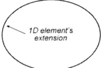
It should be noted that there is one and only one nD-element per object. This implies that some nD elements can be disconnected. In the 3D Euclidean space (R3), four types of dimensional elements are allowed, i.e. 0D, 1D, 2D and 3D elements. Fig. 2 illustrates the dimensional elements of a polygon as the order of all the points in the polygon is specified. This polygon has a 2D-element, a 1D-element and a 0D-element. The 2D-element coincides with the spatial object (i.e. the polygon). Definition 2. The nD-element of a spatial object C has an extension and may have a limit. The extension is the subset of C formed by its points of order n, and the limit is the subset of C formed by its points of order 0 to order (n 1).
Thus, if a nD-element has a limit, this limit corresponds to a lower (n 1)D-ele-ment. The 0D-element does not have a limit by definition. Note, that in the case of
Fig. 2. Order of points of a polygon and its dimensional elements. Fig. 1. Examples of simple spatial objects.
an ellipse, the 1D-element does not have a limit (Fig. 3). In contrast to the topological boundary, the limit does not necessarily enclose the extension (Fig. 2, 1D element’s limit and extension).
3.3. Framework for representing spatial relationships
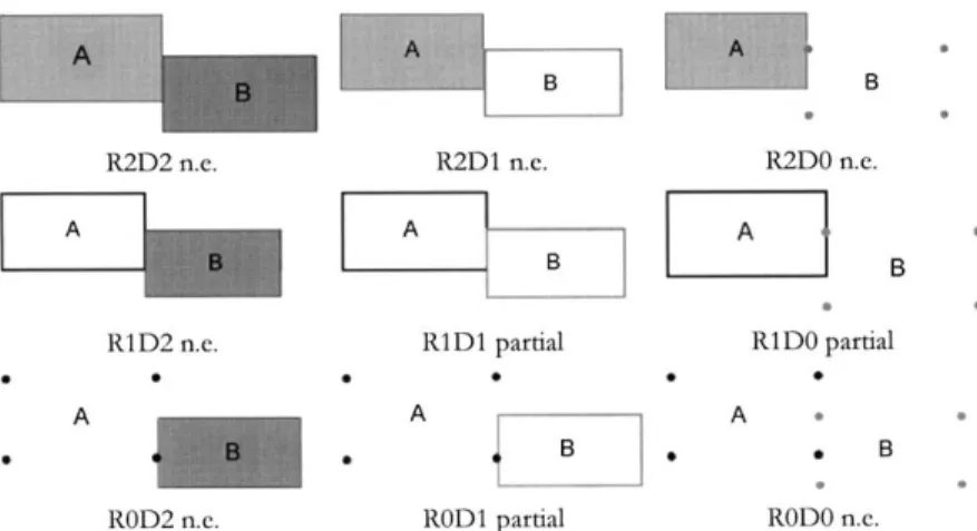
We use the dimensional elements to describe spatial relationships. We define dimensional relationships as relationships that exist between dimensional elements. The dimensional relationships are oriented, i.e. the order of the dimensional ele-ments is critical for the type of the relationship. We define three types of dimensional relationships, i.e. total (t), partial (p) and non-existent (n.e.) (Fig. 4).
Definition 3. A dimensional element is in total relation with another dimensional element if their intersection is equal to the first element, and the intersection between their extensions is not empty.
Definition 4. A dimensional element is in partial relation with another dimensional element if their intersection is not equal to the first element, and the intersection between their extensions is not empty.
Definition 5. A dimensional element is in no relation (non-existent) with another dimensional element if the intersection between their extensions is empty.
There are three groups of dimensional relationships, i.e. simplified, basic and extended. The basic relationships are the relationships that exist between every
Fig. 4. Dimensional relationships R2D2 (from black to grey 2D element). Fig. 3. 1D element without limit (closed line or ellipse’s contour).
possible combination of dimensional elements of both spatial objects. The extended relationships consider the dimension of the intersection (when it exists) between the dimensional elements. Finally, the simplified relationships are aggregation of the basic ones. They take into account the dimensional elements of only one of the objects. In R3, we have identified 12 simplified, 30 basic and 34 extended possible dimensional relationships.
To represent the basic dimensional relationships, one has to consider all the dimensional elements. For example, the dimensional relationships between two simple spatial objects of dimension 2 (i.e. polygons A and B) (Fig. 5) can be defined in the following order: first, check the dimensional relationship between 2D element of A and all the dimensional elements of spatial object B; then, check the dimensional relationship between 1D element of A and all the dimensional elements of spatial object B, etc. We denote with R—relationships, xD—dimensional element of the first object, and y—dimensional element of the second object. For example, the notation R2D1 represents the basic dimensional relationships between the 2D element of the first object and the 1D element of the second object.
Some dimensional elements might be sometimes irrelevant in a geographical point of view. Imagine that one wants to know if one cadastral parcel ‘‘touches’’ another one, no matter what is the common part (1D or 0D element). Then, it will be sufficient to consider the 1D element (without limit) and investigate only R1D1 relationships.
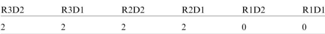
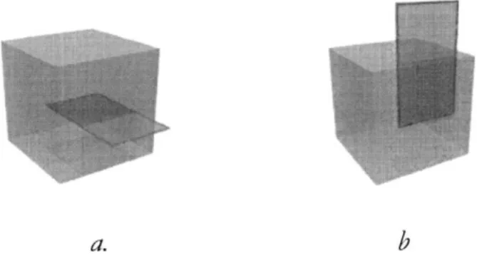
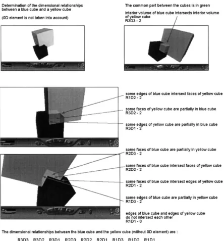
We demonstrate the basic, extended and simplified relationships by using the configuration between a cube and a polygon shown in Fig. 6a. The basic rela-tionships are obtained by looking at all the dimensional elements of the object. Using 0 for non-existent relation, 1 for total relation and 2 for partial relation, we have:
Basic relationships
R3D2 R3D1 R3D0 R2D2 R2D1 R2D0 R1D2 R1D1 R1D0 R0D2 R0D1 R0D0
2 2 2 2 2 0 0 0 0 0 0 0
To obtain the extended relationships, we look at the intersections. We can see that the relation R2D2 (i.e. between 2D element of the cube and 2D element of the polygon) is partial, but their intersection is a line segment and has dimension 1. Fig. 6b shows an example of a R2D2 partial, i.e. the intersection has dimension 2. Note, that if non-planar polygon is allowed, we may have an intersection of dimen-sion 0. We keep the code 2 for the partial relation, in which the dimendimen-sion of the intersection is equal to dimension of the lowest dimensional element considered in the spatial objects (i.e. a 2D intersection for a R2D2, a 1D intersection for a R3D1, etc.). We give code 3 when the dimension of the intersection is smaller (i.e. a 1D intersection for a R2D2, a 0D intersection for a R2D1, etc.), and a code 4 in the case of a 0D intersection for a R2D2. Thus the notations become:
Extended relationships
R3D2 R3D1 R3D0 R2D2 R2D1 R2D0 R1D2 R1D1 R1D0 R0D2 R0D1 R0D0
2 2 2 3 3 0 0 0 0 0 0 0
Finally, to use the simplified relationships, we will have an aggregation of R3D2, R3D1 and R3D0, R2D2, R2D1 and R2D0, R1D2, R1D1 and R1D0, R0D2, R0D1 and R0D0, i.e.
Simplified relationships
R3D R2D R1D R0D
2 2 0 0
If one of the dimensional elements is not geographically relevant, we can remove it from the analysis. In this case, we obtain different groups of selected relationships. For example, if 0D element is not considered, the basic relationships will become:
Selected basic relationships
R3D2 R3D1 R2D2 R2D1 R1D2 R1D1
The presented framework offers an elegant and flexible way of representing a large group of spatial relationships in 3D space. The combination of the freedom in choosing geographically relevant dimensional elements and the three groups of dimensional relationships allows one to decide on working with a very simple set of spatial relationship or on very complex (more than few hundred) ones. The DM detects all the topological relationships presented by Egenhofer and Herring (1990). A comparison between both models can be found in Billen et al. (in press).
4. Application to 3D cadastre
The 3D model is often related to only 3D visualisation as the 3D spatial querying, i.e. one of the key issues of a functional 3D GIS, is frequently underestimated. We present here the potential of 3D queries and concepts with respect to the 3D cadastral model.
4.1. Influence of the object’s representation (2D/3D) on the spatial querying
One quite common query in urban planning is to determine all the owners that are affected by geographical phenomena (pipe, road, noise pollution, etc.). The 2D solution is selecting all the cadastral parcels that are crossed or touched by the given phenomena. The 2D representation of the phenomena (e.g. road project) is super-imposed onto the cadastral object. The query is ‘‘select all the objects that have common parts’’. Actually, this is a selection of parcels based on a topological cri-terion. What is the evolution of such a query in a 3D model? One solution of extending the notion in 3D is to keep the same kind of definition, i.e. the 2D cadastral parcel (unit). This is possible because the 3D model does not impose maintenance of only 3D spatial objects, e.g. a polygon (i.e. 2D object) embedded in 3D (i.e. having 3D coordinates) has still dimension two. Suppose one wants to express the relationships to other objects under or above the ground. Then it would be necessary to either: (1) associate the distance to the other object as an attribute to the cadastral unit or (2) to compute the distance between the two objects. Note, that
the direction of the distance has to be also defined. In the first case, extra attribute information is stored, in the second case, the spatial query requires metric compu-tations (i.e. it is not a topological query). Fig. 7 shows an example of a 2D cadastral unit and an underground pipe. The query can be formulated as: ‘‘Is the pipe at a particular distance from the 2D cadastral unit’’.
Another solution is to create a new 3D object, i.e. a 3D cadastral unit that could be represented by a polyhedron. In that case, the query becomes: ‘‘Does the pipe intersect (or is included in) the 3D cadastral unit (see Fig. 7, 3D)’’. The spatial query then has the same nature as the initial query in 2D, i.e. it is a topological one. The intuitive conclusion is that 3D spatial queries are significantly important for the third dimension. This is true regardless of the choice between 2D or 3D cadastral unit. But if cadastral unit is defined as 3D object, 3D topological (or more general dimensional) relationships must be supported. Therefore, a 3D topological data structure must be contemplated as an option. Some of our developments toward this direction are presented below.
4.2. 3D segmentation of space
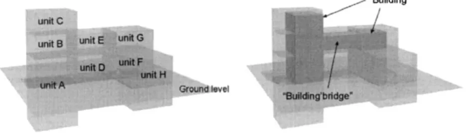
The 3D cadastral unit concept may lead to a new approach and a new division of property space. Fig. 8 illustrates a cadastral space partition. The building is built on
Fig. 8. Partition of a building.
(or in!) a private cadastral property (composed by cadastral units A, B, C, E, F and G) and a road section, i.e. municipality property (unit D). This kind of partitions would be also very interesting for utility management as sewer, pipes, etc. Obviously, these approaches require support of 3D spatial relationships and 3D spatial objects.
4.3. The dimensional model and spatial analysis
As presented in Section 3.3, the dimensional relationships allow working with a very simple or very complex set of spatial relationships. In the cases of spatial queries mentioned above, these different complexity levels may lead to either sim-plified or very precise descriptions of the relationships between spatial objects. For some queries, the simplified relationships are sufficient. Let us consider the impact of a noise pollution on cadastral units (Fig. 9a). If a 2D spatial object (e.g. a polygon) represents the noise pollution, the only dimensional relationship of interest is R2D2. Indeed, it is irrelevant to refine the spatial relationships at the level of 1D or 0D element. The question is whether the cadastral unit is affected by the noise pollution, as the exact relationships between the borders (edges and corners) are not of interest. In addition, the object ‘‘pollution’’ has rather approximate extension. However, some complex spatial queries could be necessary when all the dimensional elements play a role, e.g.:
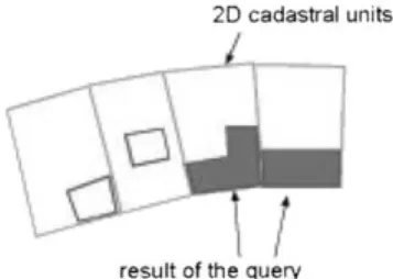
Find all the buildings that lay on at least one edge of the cadastral unit. This query requires to determine if the R2D2 is total, R1D1 partial and R0D0 partial (Fig. 9, 2D example);
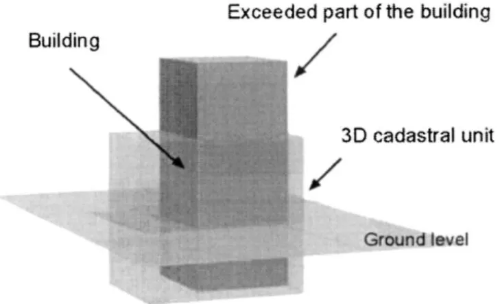
Find all the buildings that exceed the cadastral limit and determine the exceeded part.Expressed by R3D3 partial (example given in 3D). The exceeded part can be retrieve by analysing the relationships between the lower dimensional elements of both objects (2D, 1D and 0D element) (Fig. 10).
In both cases, The Dimensional model provides an appropriate answer to the question. See Section 5 for some queries performed in the Oracle database.
4.4. Data consistency
One of the major challenges for cadastral administration has always been quality and consistency of data. The consistency of the topological relationships between objects is often considered the major criterion for the quality of the model. The examples discussed above referred to the interaction between cadastral objects and other objects (topographic or fictional). But spatial relationships exist also between cadastral objects. For example, an important task of cadastre is to classify the land following a property criterion. By definition, a piece of land may not belong to more than one cadastral unit and all parts of the modelled space belong to exactly one cadastral unit (or are on the border). This could be controlled by topological rela-tionships between all the cadastral units, i.e. a cadastral unit may not intersect another one. This query can be easily expressed in dimensional terms, i.e. dimen-sional relationship between higher dimendimen-sional elements of two cadastral units (2D or 3D) must be non-existent. In case of a 3D cadastral unit, the relationship will be R3D3 (n.e.) and in case of a 2D cadastral unit R2D2 (n.e.).
It is evident that if 3D cadastral models are envisaged, adapted 3D topology structures (and by extension 3D dimensional structures) have to be adopted. Fur-thermore, there are different types of inconsistency in spatial data. In this research, we are only interested in the topo-semantic ones, which concerns topological rela-tionships between objects according to their semantic definition. Fig. 11 portrays examples of 2D and 3D topo-semantic consistency.
5. Implementation and tests
To be able to test the presented Dimensional model in detecting spatial relation-ships, we have selected a spatial model to describe spatial objects. A large number of spatial models are developed and implemented in GIS, Computer Graphics and CAD systems based on irregular multidimensional cells (Egenhofer, Frank, &
Jackson, 1989; Ma¨ntyla¨, 1988; Molenaar, 1990; Pigot, 1995; Pilouk, 1996; Zlata-nova, 2000). The names and construction rules of the cells in the different models usually vary. The simplest set of cells is the set of simplexes, i.e. 0-simplex (node), 1-simplex (arc), 2-1-simplex (triangle) and 3-1-simplex (tetrahedron). Most of the models allow 1,2,3-cells with an arbitrary shape that imposes some supplementary
Fig. 11. Topo-semantic inconsistencies.
constraints, e.g. planarity of faces, convex shape (Molenaar, 1990; Pigot, 1995; Zla-tanova, 2000). The names node (vertex, point), edge, face (polygon) and body (solid, polyhedron)are then used in the literature to denote 0,1,2,3-cell. Furthermore, the models can be classified into spatial models with explicit representation of objects and spatial models with explicit representation of spatial relationships (topology). Each of the models has advantages and disadvantages that are not to be discussed here. We have concentrated on the Simplified Spatial Model (SSS; Zlatanova 2000) basically due to four reasons. First, the model is a typical example of an explicit representation of objects, which suits our conceptual model. Second, the model has been tested with the framework of Egenhofer for representing spatial relationships that provides a basis for comparison between the two frameworks. Third, the model maintains minimal elements (i.e. node and face) for describing spatial objects and thus simplifies the reconstruction of 3D objects. Fourth, the model has been suc-cessfully tested for large 3D models (of size than can be expected for urban models). We have implemented the concepts of the dimensional model as operators in Oracle database and have tested these operators with two data sets organised
according to the construction rules of SSS. The operations are developed with the high level programming language (an extension of SQL) provided by Oracle, i.e. PL/ SQL. To be able to visualise results of the queries, a VRML file is created on the fly with the objects of interest and the intersecting parts.
With these dimensional operators, it is practically possible to retrieve basic dimensional relationships between body and body, body and face, body and point, face and face, line and line. The dimensional query returns an answer in a form of relational table that contains all the existing dimensional relationships. Other operators have been developed to extract the precise geometry of the ‘‘potential’’ intersection between spatial objects. Thus, we can obtain the complete description of the spatial relationship between two spatial objects and also its correct 3D geometric representation. The 3D visualisation is achieved via a Java program that translates the Oracle table into a VRML file.
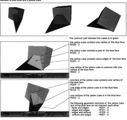
The tested queries are: (1) what is the spatial relationship between two bodies? (Fig. 12) and (2) what is the spatial relationship between a body and a polygon? (Fig. 13). In the program, numbers decodes the types of relationships, i.e. 0—non-existent, 1—total, and 2—partial.
6. Conclusion and future developments
The final objective of 3D GIS is to have a complete 3D model of the reality for topographic and fictional objects. It seems judicious to envisage real 3D concepts for the cadastre by the evolution of the notion of cadastral parcel (2D space partition) to the extended notion of a 3D cadastral unit. Whatever 2D or 3D cadastral objects will be practically selected, a certain level of 3D spatial analysis must be reached. Either topological data structures should be used or 3D spatial operators for non-topological data structures have to be developed. In both cases, the Dimensional model can be used as a framework for the management of 3D spatial relationships. In near future, we will continue experiments with SSS and other data structures toward development of more elaborated 3D spatial queries.
References
Billen, R., Zlatanova, S., Mathonet, P., & Boniver, F. (2002). The Dimensional Model: a framework to distinguish spatial relationships. In: D. Richardson, & P. van Oosterom (Eds.) Advances in Spatial Data Handling, (pp 285–298). Berlin: Springer-Verlag.
Clementini, E., di Felice, P., & van Oosterom, P. (1993). A small set of formal topological relations sui-table for end-user interaction. In Proceedings of the 3th International Symposium on large spatial data-bases(pp. 277–295). Berlin: Springer-Verlag.
Danahy, J. (1997). A set of visualisation data needs in urban environmental planning&design for photo-grammetric data. In Proceedings of the Ascona Workshop ’97: automatic extraction of man-made objects from aerial and space images(pp. 357–365), Monte Verita, Switzerland.
Egenhofer, M. J., Frank, A. U., & Jackson, J. P. (1989). A topological data model for spatial databases. NCGIA Technical report, No. 104.
relationships. In Proceedings of Fourth International Symposium on SDH (pp. 803–813), Zurich, Switzerland.
Fuchs, C. (1996).OEEPE study on 3D city models. Report of the Institute for Photogrammetry, University of Bonn, October.
Gru¨n, A., & Dan, H. (1997). TOBAGO—a topology builder for the automated generation of building models. In Proceedings of the Ascona Workshop ’97: automatic extraction of man-made objects from aerial and space images(pp. 149–160), Monte Verita, Switzerland.
Leberl, F., & Gruber, M. (1996). Modelling a French village in the Alps. In Proceedings of the 12th Spring Conference, Budmerice, Slovak Republic.
Ma¨ntyla¨, M. (1988). An introduction to solid modelling. New York, USA: Computer Science Press. Molenaar, M. (1990): A formal data structure for 3D vector maps. In Proceedings of EGIS’90, Vol. 2 (pp.
770–781), Amsterdam, The Netherlands.
Pantazis, D., & Donnay, J.-P. (1996). La conception de SIG, me´thode et formalisme. Paris, France: Herme`s.
Pigot, S. (1995). A topological model for a 3-dimensional spatial information system. PhD thesis, University of Tasmania, Australia.
Pilouk, M. (1996). Integrated modelling for 3D GIS. PhD thesis, ITC, The Netherlands.
Pullar, D. V., & Egenhofer, M. J. (1988). Toward formal definition of topological relations among spatial objects. In Proceedings of the Third International symposium on SDH (pp. 225–241), Sydney, Australia. Ranzinger, M., & Gleixner, G. (1995). Changing the city: data sets and applications for 3D urban
planning. In GIS Europe (pp. 28–30), March.
Tempfli, K. (1998). Urban 3D topologic data and texture by digital photogrammetry. In Proceeding of ISPRS, March-April, Tempa, Florida, USA, CD-ROM.