Advanced capabilities for the simulation of membrane and inflatable space structures using SAMCEF

Advanced capabilities for the simulation of membrane and

inflatable space structures using SAMCEF

Philippe Jetteur1 and Michaël Bruyneel2 1,2

Samtech s.a., Liège Science Park, Rue de Chasseurs-Ardennais 8, B-4031 Angleur, Belgium philippe.jetteur@samcef.com michael.bruyneel@samcef.com

1 Introduction

SAMCEF Mecano is a general implicit non-linear software developed by Samtech [1]. For the past two years, several improvements have been made in SAMCEF Mecano concerning the analysis of inflatable and membrane structures. Most of the developments have been carried out under an ESTEC contract, in the frame of PASTISS project – Professional Analysis Software Tool for Inflatable Space Structure [2,3,4].

The developments cover different aspects. In this paper, we give a general overview of the different capabilities.

The first point concerns the choice of the finite element. We have chosen a shell without rotational degrees of freedom as main element for this kind of application. Because there is no bad conditioning with it, the stiffness matrix becomes equal to the one of a membrane element when the element is very thin. The second point is related to the strategy of resolution. Since a classical Newton-Raphson strategy is not well suited for this kind of structure, we present several alternatives.

The other topics are related to a material without resistance in compression, to the measure of the internal volume, to the production of gas, to the definition of the initial free geometry, to the computation of eigenvalue…

2 Shell without rotational degrees of freedom

In an inflatable structure, the thickness is very small. If classical shell elements are used, numerical difficulties arise because the order of magnitude of the stiffness terms linked to translational degrees of freedom is very different from the one linked to rotational degrees of freedom. An alternative consists in using membrane elements but, in this case, it is not possible to get the wrinkling pattern and the computation is less stable. The solution is to use a shell without rotational degrees of freedom: when the thickness becomes very small the stiffness matrix becomes similar to the one of a membrane element.

The element is closed to the one described in [5,6].

2.1 Flexural behavior

For the flexural behavior, we start from a triangle where the unknowns are the translational displacements of the corner nodes and the rotations around the edge. The curvature and the moment are constant over the element. This last can be seen either as a non-conforming displacement element or as an equilibrium element. This is a Kirchhoff plate element. It is a classical element. The flexural energy can be written as:

{ }

From these 6 degrees of freedom, we can extract 3 rigid body modes and 3 deformation modes. As deformation modes, we take α, the difference between the rotation around the edge and the rigid rotation. In the element without rotational degrees of freedom, we compute α as a function of the positions and displacements of a patch of elements (Fig. 1). We look at edge AB of the triangle. C is the third point of the triangle and D is a point of the patch of elements.

Fig. 1. Patch of elements, computation of the relative rotation

The relative angle between the 2 triangles is easily computed. In nonlinear analysis, the moments depend on the current value of α minus the initial value.It is worth noticing that, as the relative rotation around the edge is a scalar, we do not have any problem with large rotation in nonlinear analysis. As the rotation is not computed by an updated procedure, the solution does not depend on the size of the time step for nonlinear static analysis with linear material, as far as convergence is reached.

Special treatment is needed at the boundary. See [7] for the adopted solution.

2.2 Membrane behavior

For the membrane behavior, we follow the solution adopted in [6]. First, the strains are computed on the element patch as for a 6 node triangular element. Then, we compute the mean strain on the central triangle. With this procedure, the membrane behavior is much better than the one of a constant strain triangle and is nearly similar to the one of a second order element.

2.3 Numerical example

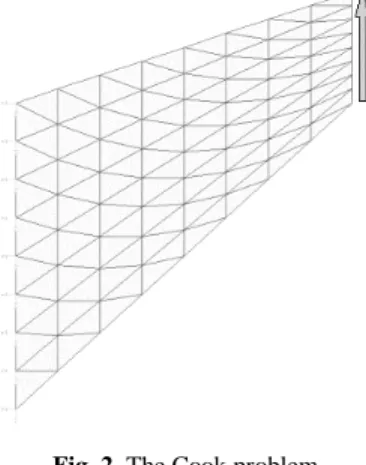
The first example is a classical linear problem (Cook problem, see Fig. 2). In this test, we only study the membrane behavior and we compare the developed element to classical first order (constant strain triangle) and second order elements.

Fig. 2. The Cook problem

From Table 1, it can be seen that the solution obtained with the present element is much better than the one obtained with a classical first order element, which has the same number of degrees of freedom.

Table 1. Results for Cook problem. Displacement associated to the load

1st order 2nd order Present element

2*2 11.97 26.28 22.72

4*4 18.26 26.03 24.54

8*8 22.00 25.37 24.24

16*16 23.41 24.82 24.10

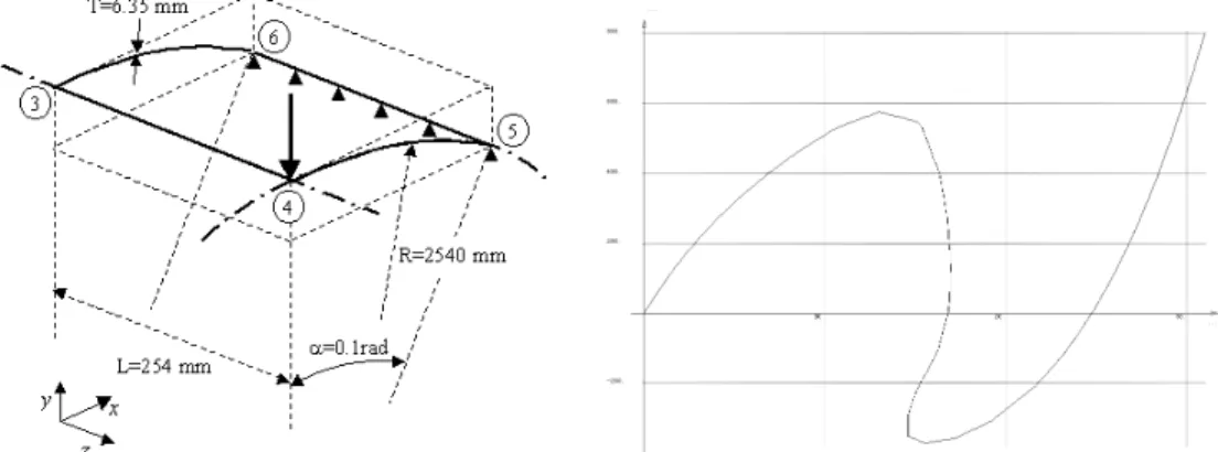
The second example is a classical non linear shell problem. It studies the snap-through of a cylindrical shell (Fig. 3). The straight edges are pinned and the curved edges are free. Only a quarter of the model is considered. We look at the curve external force / displacement under the load (Fig. 3). The result is similar to the one obtained with classical shell elements.

Fig. 3. Snap through of a cylindrical shell

3 Resolution methods

It is well established (see for example [8,9,10]) that using a Newton-Raphson approach for determining the structural shape during a slow inflation process can lead to large oscillations and lacks of convergence. The difficulty comes from the small stiffness of the membrane in the transversal direction. As soon as there is a little compression in the structure, wrinkles appear. There are several equilibrium states which have nearly the same energy but have different buckling patterns. The buckling pattern can change in function of the load factor. The convergence of a classical Newton-Raphson scheme becomes difficult. To circumvent this difficulty, an explicit scheme can be selected [9], that provide some inertia avoiding large movements of the nodal positions. Since it requires tuning of damping parameters, undesirable dynamical effects can occur, leading to a non realistic inflation process simulation.

We developed 3 kinds of approaches in order to find the equilibrium states in an implicit way. In the first one, we compute the energy of the system and we look for the minimum of energy, using an optimization approach. In this case, a Newton-Raphson scheme is not used. In the second approach, we modify the Newton-Raphson scheme: we do not iterate with a tangent matrix, but we skip some terms in this matrix in order to stabilize the iterations. In these two approaches, an equilibrium is reached. It is not sure it is linked to a global minimum of the energy, it can be a local one. In the third approach, we perform a Sturm sequence at the end of each step to be sure that the solution is stable. We reduce the size of the time step if it is not stable and we add dynamic effects in order to go from one pattern to another one.

3.1 An optimization approach for the inflation process simulation

Comparison between the Newton-Raphson and the optimization schemes

In both numerical schemes, the variable nodal positions are updated according to the following rule, ) ( ) (k k 1) (k _{q αs} q + = +

where q(k) is the vector of positions at the actual iteration k, while q(k+1) is the updated vector. Those new positions are obtained for computed search direction s(k) and step length α. Calculating the parameter α is known as the line search procedure.

In the Newton-Raphson approach, the search direction is computed based on the tangent stiffness matrix (second order information). It involves the solution of successive linear approximations of the equilibrium equations, with all the difficulties that can be related to it, as an ill-definiteness of the tangent matrix that often occur in the problem under interest. A unit step length α=1 is classically considered, although some line search capabilities are sometimes available.

In the optimization approach, we rather try to find the minimum of the total potential energy of the system. Since several optimization techniques exist, a right method selection can be made according to the problem’s features. For example, using a first order minimization technique will avoid any troubles with a possible ill-definiteness of the tangent matrix. Additionally, different ways for computing the descent search direction could be easily combined.

Considered optimization problems

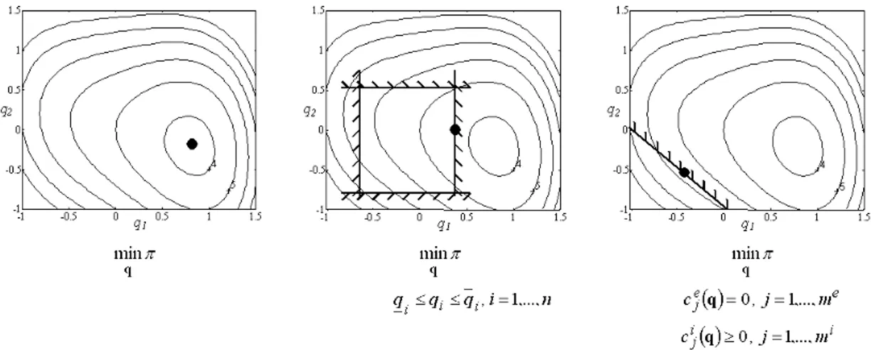
The three kinds of optimization problems are reported in Fig.4, namely unconstrained, quasi-unconstrained and constrained optimizations. π is the objective function to minimize over the values q={qi, i=1,n}.

Fig. 4. Three kinds of optimization problems: unconstrained, quasi-unconstrained and constrained

In the frame of inflated structures, the nodal positions (displacements) are the unknowns. Looking at the minimum of the total potential energy π will lead to the (an) equilibrium state. In this case, an unconstrained optimization method is needed. When the value of some degrees of freedom is restricted, or when some of them are linked, the problem becomes constrained, and Lagrangian multipliers characterize the activity of those restrictions. Such formulations are used when rigid body elements are considered, or when the problem includes contact conditions. In this case, a constrained or quasi-unconstrained optimization method is necessary.

Optimization strategy for inflated structures [10,11]

Since general constrained optimization problems must be solved, a constrained optimization technique must be considered. Different optimization methods are available: Sequential Convex Programming [12,13], mathematical programming [14,15,16], etc. After a tests campaign [13], the augmented Lagrangian method was found to be appropriate and reliable (Fig. 5).

Fig. 5. Iterative augmented Lagrangien optimization method. The solution of the constrained optimization problem is

In this approach, belonging to the sequential unconstrained minimization techniques, the solution of the initial constrained optimization problem is replaced by the solution of successive approximated unconstrained minimization problems (approximated in the sense that the Lagrangian multipliers and the constraints are only exact and satisfied at the solution). The development of such a technique requires two steps described below. The constrained optimization method

The way to transform a constrained optimization problem into an unconstrained one, which includes the evaluation of the Lagrangian multipliers, is described here. The optimization problem writes:

π q min subject to ce_j

( )

( )

( )

( )

( )

( )

( )

( )

The Lagrangian multipliers λλλλ associated to the constraints are updated with a simple but efficient steepest ascent approach in the dual space [17], by comparing the optimality conditions of the augmented Lagrangian function with the stationarity conditions at the optimal solution. It comes that:

j j new

j k pc

kλ = λ + with λ_j ≥0, j=1,...,mi

For the inequality constraints, the dual variables must always be positive; for equality constraints, their sign is not restricted. In our applications k=p, and only equality constraints have to be considered.

The unconstrained optimization problem

The conjugate gradient method is selected. It aims at solving the following quasi-unconstrained minimization problem:

f

q

min subject to q_i≤qi≤q_i i=1,...,n

where f is a general non linear function. Here, f = La is the augmented Lagrangian function given above. This is a

first order method, that is the tangent matrix doesn’t have to be computed. The search direction is given by, ) 1 ( ) 1 ( ) ( ) (k _=−gk _+βk− _sk− s

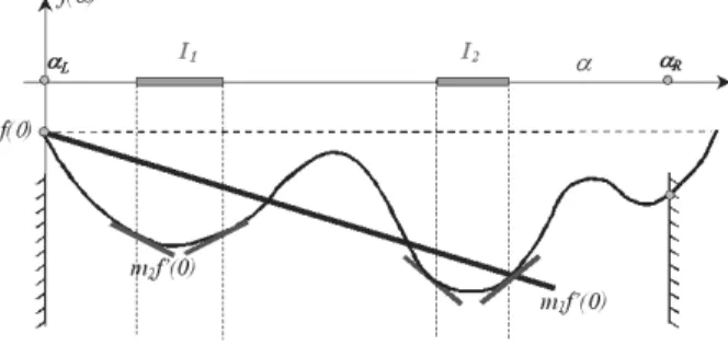
where the scalar β is the conjugacy parameter. The step length α is computed with a line search based on a cubic interpolation in the general frame of the Wolfe conditions [10,16]. For saving computational time, this line search process is not exact: only an approximated minimum is looked for along the computed search direction (Fig. 6). Since the function f is not quadratic over the nodal positions q, and as the line search is not exact, the conjugacy parameter β is computed with the Hestenes-Stiefel formula [14,15,16].

Features of the developed optimization method and recommendations

When the optimization method is used, slow convergence can occur for large scale problems, that is with more than 105 degrees of freedom. Given that the second order information (tangent matrix) is not used, the quadratic termination of the Newton-Raphson solution scheme is lost. A second reason for slow convergence is

related to the iterative process required for updating the Lagrangian multipliers in a constrained optimization problem.

Additionally, it should be noted that some theoretical limitations exist regarding the use of a potential function related to the pressure. It is impossible to find a solution when free edges appear in the structure, that is the inflated structures must be closed.

Fig. 6. The Wolfe conditions defining an approximated minimum along the search direction.

Good candidates are located in the sets I1 and I2

Numerical example

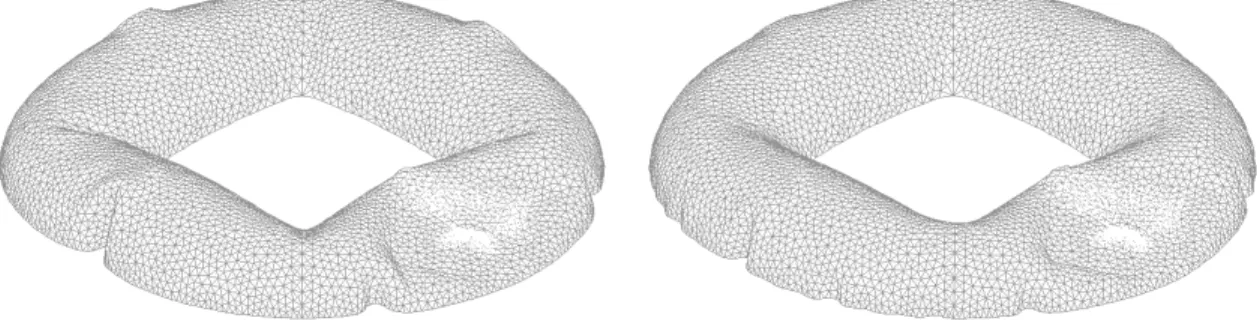
In this section, an initially flat circle lifesaver with an internal square outline is considered. The model includes 14222 degrees of freedom. The shapes for two different pressure levels are reported (Times 0.5 and 1). As the problem is symmetric, only the upper half of the structure is considered. Four different inflation situations are investigated. The first problem doesn’t include any nodal restriction (Fig. 7). In the second one, the vertical displacement of a quarter of the set of nodes is limited to an upper value (Fig. 8). In Fig. 9, a flat rigid part is modeled: the nodes lying in this part must stay in the same plane during the inflation process (what leads to 990 equality constraints in the optimization problem). Finally, the contact between the inflated structure and a rigid sphere is studied in Fig 10 (1101 equality constraints).

Fig. 7. Solution without any nodal restrictions for 2 successive pressure levels

Fig. 9. Solution with a RBE for 2 successive pressure levels

Fig. 10. Solution with a contact condition for 2 successive pressure levels

3.2 Modified Newton-Raphson scheme

Principle

During the iterations, some compression appears in the structure. The iteration matrix is no more definite positive. The variation of the displacement during one iteration can be very large and convergence is not reached.

A classical modification of the Newton-Raphson scheme is to iterate with a constant matrix. This modification is mainly done for performance not for convergence problem.

If we look at the tangent matrix of the element, there are two parts. The first one is proportional to the Hooke law and takes also into account large rotations of the elements. The second one is proportional to the state of stress and is called geometric stiffness. We look at the terms in the geometric stiffness which depend on the normal forces. In the modification we perform, we only take into account the positive normal forces in the geometric stiffness. As we do not have a tangent matrix, we increase the number of allowable iterations during a time step. The convergence is not quadratic.

Numerical example

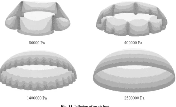
As example, we simulate the inflation of an airbag. We start from a flat disk and we apply a pressure on it. Figure 11 shows the deformation for different values of the pressure

The first difficulty is at the beginning of the analysis because there is nearly no transversal rigidity before there are some traction forces in the membrane. The size of the first time step is automatically chosen in such a way that at the end of the first iteration, which is equivalent to a linear analysis, the rotations are smaller than a given value (0.2 rad for instance). Once a pressure is present, there is a traction normal force and so there is a transversal stiffness.

The next difficulty is when the number of waves along the circumference changes. Several iterations are needed and the convergence is not uniform. In this method, we check that the solution is in equilibrium, but we do not check that it corresponds to a global minimum of energy.

Fig. 11. Inflation of an air bag

It is seen from the results that the wave length decreases when the pressure increases. At the end, the structure is very stiff and convergence is easy to reach. If membrane elements are used instead of shell elements, the buckling pattern is less smooth.

3.3 Buckling pattern

Principle

In this case, we want to have the buckling pattern which corresponds to a global minimum of energy. At the end of the step, when the convergence is reached, we perform a Sturm sequence on the iteration matrix. If some eigenvalues are smaller than 0, it means that the structure is un-stable and that there is another configuration with less energy. The time step is rejected and a new time step is restarted with a smaller value.

In this kind of structure, this configuration is created by a change in the buckling pattern. We have to go from a configuration to another one, which may be not connected in such a case. A classical Riks like method is not sufficient [18]. In order to go from one branch to another one and to get convergence, we add inertia terms. As we are not interested in the dynamic effects, we use a Newmark scheme with non-standard value for β and γ. We choose values which give a large numerical damping but for which the scheme is un-conditionally stable.

In order to be simple, we keep this scheme during the whole analysis. It can be checked in post-processing that the inertia forces and the kinetic energy is negligible except when there is a mode change.

Numerical example

As example, we take a rectangular plate subjected to shear [19]. Figure 12 shows isovalue of transversal displacement for different load level. It can be seen that the number of wrinkles increases with the loading, and that the wave length decreases. A small geometrical imperfection is introduced.

4 Equivalent material

In inflatable structures, the thickness of the membrane is very thin with respect to the other dimensions. The buckling loads are very low and wrinkles appear. But the post-critical path is stable. Depending on the application, it is important to have a good numerical prediction of these wrinkles. In this case, a very fine element mesh is needed, like in the previous example. In some cases, only the global behavior of the structure is looked at, and it is not important to simulate the wrinkle pattern. In this chapter, we deal with these cases.

In order to take into account the buckling, the constitutive law is changed. It is assumed that the material has no resistance in compression. Using an implicit solver with a Newton Raphson scheme, if the resistance in compression is equal to zero, convergence problems can arise, especially if the two principal directions are in compression. In order to improve the convergence, we introduce a small resistance in compression. The difficulty with this resistance in compression is the interaction between the two directions due to Poisson effect, in order to have a continuous response between the different states of stresses (traction/traction, traction/compression, compression/compression). We define a stress potential in order to specify the material behavior.

We restrict the analysis to isotropic material for which the principal stresses and strains are parallel.

4.1 Theoretical aspect

We start from the behavior in principal axes and we define a stress potential in function of the 2 principal stresses:

( )

( )

[

]

In case of a standard elastic material with a resistance in compression, F will be a quadratic function of the stress (F = σ2/2). We now consider a material where the modulus in traction is E and where the modulus in compression is smaller (kE, k<<1). The F function is taken equal to:

k F then if F then if 2 0 2 0 2 2 σ σ σ σ = < = ≥

We can now look at the different cases. In case of traction in both directions, we get the standard elastic material. In case of a traction / compression behavior, we have:

2 1 2 2 1 2 1 2 1 2 1 2 1 2 1 1 1 1 1 1 1 : 0 , 0 ε ε ν ν ν σ σ σ σ ν ν σ νσ νσ σ ε ε σ σ k k k k E k E k E − = ⇒ − − = + − − = < >

When k becomes small (equal to 0), we find an uniaxial behavior. With this bilinear behavior, we have a small stiffness in compression. No singularity arises when the stiffness in compression becomes equal to 0. The behavior is continuous when the state of stress goes from a traction/traction state to a traction/compression state or to a compression/compression state. There is a slope discontinuity at the origin. One way to have a smooth transition between traction and compression is to change the F function. The curve corresponding to the derivative of F will have E as slope for a large positive strain and kE for a large negative strain.

Once the material behavior is well defined in principal axes, it is easy to define it in XY axes as the principal axes for the stress tensor and the strain tensor are identical and as there is no history in the constitutive law. For the stresses and strains, nothing special must be said. In the tangent constitutive law, we take into account the rotation of the principle axes. More details on the equations can be found in [20].

4.2 Numerical example

We use a static implicit scheme; no mass is taken into account. A Newton scheme is used in order to reach the equilibrium.

As element, we use the shell without rotational degrees of freedom. The material without resistance in compression is used for the membrane behavior. The flexural behavior is classical. The flexural behavior helps the convergence at the beginning of the analysis when the traction in the element is low. When the traction becomes large, as the shell is very thin, the flexural behavior becomes negligible.

The example is an airbag inflation. The initial geometry is circular, the radius is equal to 0.35, the thickness to 0.0004, the Young modulus to 6Χ107, the Poisson ratio to 0.3 The applied pressure is equal to 5000.

A reference solution is made with a fine mesh (20000 elements) with a classical elastic material. Figure 13.a shows the deformed shape, the mean principal membrane stresses are plotted on Figure 13.b.

Fig. 13. Reference mesh, a) deformed shape, b) principal stresses

Two coarse meshes are build. One with 310 elements and one with 35 elements. Figure 14.a shows the principal stresses results obtained with the classical material and Figure 14.b with the material with a small resistance in compression. We take a module equal to 6Χ104 in compression. Without any resistance in

compression, convergence is difficult to obtain in a static analysis. Table 1 provides the central displacement for the different solutions. It can be seen that the solution with the material with the small compression is very stable and is close to the solution obtained with the fine mesh and the classical material.

Table 2. Central displacement

20000 elements 310 elements 35 elements Classical material 0.175 0.173 0.165 Small compression 0.175 0.175 0.175

5 Volume measure

In inflatable structures, it is often important to know the internal volume and to have a relation between the internal volume and the internal pressure. One solution is to use fluid elements and to perform a fluid-structure interaction. Generally, especially in static analysis, this kind of solution is not needed. We adopt a cheaper solution.

We compute the internal volume by a boundary integral, using the shell mesh as boundary. The volume is linked to one additional degree of freedom. The force conjugated to this degree of freedom is a pressure. Either we can prescribe a value to this degree of freedom in function of time (internal volume imposed), or we can apply a force (internal pressure imposed) or introduce a special law on it (relation between pressure and internal volume).

The volume is computed by the following equation:

(

)

We introduce a kinematic constraint with a Lagrange multiplier. A classical Lagrangian approach is used, the Lagrange multiplier is equal to the internal pressure. This constraint links all the degrees of freedom and gives a large equation in the iteration matrix. As the nature of the degree of freedom (volume) is different from the one of the shell element (translation), it is important to scale the equations before solving them.

An example of relation between pressure and volume which is introduced is the relation for perfect gas, either isothermal or adiabatic. We introduce a non-linear spring where the force is the pressure and the displacement the volume. For the isothermal case, with a constant mass of gas, the equation is written (0 linked to the initial value) :

V

V

p

p

=

In dynamic analysis, this global representation of the fluid is a rough approximation as the pressure is constant on the whole volume.

6 Gas production

In general, in inflatable structure, the mass of gas is not constant. There is a production of gas during the inflation. If U is the gas internal energy, Q the applied heat, T the gas temperature in the cell, Tin the temperature

of the gas flowing in the cell, k the ratio between the specific heat at constant pressure and at constant volume, the gas balance of energy can be written [21]:

(

)

( )

(

)

For an adiabatic transformation, we have:

(

)

(

)

p V

kp &+ & = −1 &

For a isothermal relation, we have:

T r m V p V

p &+& = &_in

In both cases, it is a differential equation between the internal volume, the internal pressure and the flow of gas. A special one degree of freedom element is written in order to take into account these equations. As input of

the element, we have all the values at time step n, the volume at time step n+1 and its derivative in function of time. Inside the element, we use an implicit Euler scheme in order to find the pressure at time step n+1.

Similar formulas are also introduced in order to take into account a leakage of the cell.

6.2 Numerical example

As example, we take the inflation of a cushion. Initially, the geometry is similar to a flat rectangle. In order to avoid to use a fine mesh in the corner, we use a material with a small resistance in compression in order to simulate the buckling. The flow of gas is decreasing linearly with the time. As results, we plot the final shape and the evolution of the volume in function of time (Fig. 15).

Fig. 15. Inflation of a cushion

7 Activation of boundary condition

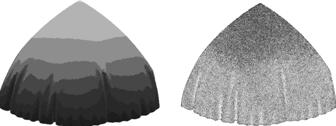
In membrane structure, what is known is the flat geometry. In order to fix the idea, we take as example a gore of a stratospheric balloon and we try to find the initial shape subjected to gravity and hydrostatic pressure. As we study only one gore, we have to introduce symmetry conditions.

We perform the computation in two steps. In the first step, we start from the flat definition of the gore, we apply the hydrostatic pressure and the gravity. The bottom and the top of the gore are fixed and the symmetry conditions are not taken into account.

In the second step, the top of the balloon is free and we introduce the symmetry conditions. The symmetry conditions are introduced through kinematic constraints with Lagrange multipliers. In order to improve the convergence and to avoid discontinuity in the response, we compute the initial value of the constraint Φ0 at the end of the first step and we impose it to be equal to 0 at the end of the activation. If tb and te are the time at the beginning and the end of the activation, the kinematic constraint during the activation is written in function of time as:

( )

In order to free the top of the displacement in a progressive way, the software applies automatically the reaction force linked to the fixation of the top as an external load and reduces it in function of time. At the end of the activation, this external force is equal to 0.

At the end, the symmetry conditions are fulfilled. Fig. 16a shows the initial shape, the shape at the end of the first step and the final shape. The meridian stresses at the end are shown in Fig. 16b.

8 Reference to a free mesh

In the previous section, we use the flat shape as geometry and we apply the boundary condition in a progressive way. There is an alternative. We define two meshes, one which respects the boundary conditions and one which corresponds to the flat shape. Practically, there are two series of nodes which are linked to the same

element. When we compute the strains, the nodes which correspond to the first mesh are seen as a deformed configuration and the nodes corresponding to the second mesh are seen as the initial configuration. If the first mesh is physically free of stresses, we find zero strains because there is only a rigid body mode between the two configurations in this particular case.

Fig. 16. One gore problem

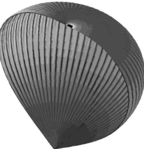
As example, we take the same stratospheric balloon as in the previous example, but half a balloon is studied. As first mesh (the one witch respects the boundary condition), we take the results of the previous example, which is rotated for each gore. As second mesh (free mesh), we take the initial mesh of the previous example. In a first step, we apply the hydrostatic pressure and the gravity load. We get immediately the convergence. In a second step, we apply a transversal force. The meridian stress distribution at the end of the computation are illustrated in Fig. 17.

9 Eigenvalue computation

The non-linear computation of the structure is one thing. At the end of the computation it is possible to extract the tangent stiffness and the mass matrix in order to perform a linear computation around a non-linear state. This linear computation is valid only if the variation of displacement is small. The linear computation could be a static analysis, a eigenvalue analysis, a transient dynamic analysis or the creation of a super-element

As example, we use the ISIS solar shield [22]. In the non-linear run, a state of traction is introduced by a prescribed transversal displacement of the centre of the shield, gravity is taken into account. As we are interested in the global response, not the wrinkling pattern, we use a material with a small resistance in compression.

Fig. 18 shows the transversal displacement of the first mode (eigenfrequency 2.26Hz). The displacement is located at the edge of the structure.

Fig. 18. Isis solar shield

10 Conclusion

Several specific facilities of the SAMCEF finite element code related to membrane and inflatable structures were presented. The developments, carried out in the frame of an ESTEC project called PASTISS, cover different aspects of the problem, i.e. selection of a convenient finite element and devising of reliable solution strategies. Some other topics were also investigated: material without resistance in compression, the measure of the internal volume, the production of gas, the definition of the initial free geometry and the computation of eigenvalue. Examples were provided and demonstrated the ability of SAMCEF in efficiently solving the problems under interest.

Acknowledgment

The main part of the development has been carried out under the contract ESA 18043/04/NL/PA “Professional Analysis Software Tool for Inflatable Structures” (GSTP program).

References

1. SAMCEF: Système d’Analyse des Milieux Continus par Eléments Finis. Samtech, Liège, Belgium. www.samcef.com 2. Jetteur P., Granville D. (2004). Finite element analysis of inflatable space structures using SAMCEF. Second European

Workshop on Inflatable Space Structures, June 21-23, Tivoli, Italy.

3. Jetteur P., Granville D. (2004). Presentation of the PASTISS project. Second European Workshop on Inflatable Space Structures, June 21-23, Tivoli, Italy

4. Bruyneel M., Jetteur P., Granville D. (2005). First results of the PASTISS project – Professional Analysis Software Tool for Inflatable Space Structures. European Conference of Space Structures, Materials and Mechanical Testing, May 10-12, ESA/ESTEC, Noordwijk, The Netherlands.

5. Guo Y.Q., Batoz J.L., Naceur H., Gati W. (2000). Two simple triangular shell elements for spring back simulation after deep drawing of thin sheets. Finite elements: techniques and developments. Proceeding of the 5th Int. Conf. On Comp. Struct. Technology, Leuven.

6. Flores F.G., Oñate E. (2005). Improvements in the membrane beahavior of the three node rotation-free BST shell triangle using an assumed strain approach. Comput. Meth. Appl. Mech. Engng 194: 907-93.

7. Jetteur Ph. (2003). Thin membrane element for inflatable structures. In: Oñate E., Kröplin B. (eds). Textile Composites and Inflatable Structures, Structural Membranes 2003. CIMNE, Barcelona.

8. Bouzidi R., Le van A. (2004). Numerical solution of hyperelastic membranes by energy minimization. Computers & Structures 82: 1961-1969.

9. Troufflard J., Cadou J.-M., Rio G. (2005). In: Oñate E., Kröplin B. (eds). Numerical and experimental study of inflatable lifejackets. Textile Composites and Inflatable Structures, Structural Membranes 2005. CIMNE, Barcelona.

10. Bruyneel M., Jetteur P., Granville D., Langlois S., Fleury C. (2005). An augmented Lagrangian optimization method for inflatable structures analysis problems. Sixth World Congress of Structural and Multidisciplinary Optimization, May 30-June 3, Rio de Janeiro, Brazil. Submitted to Structural and Multidisciplinary Optimization.

11. Bruyneel M., Jetteur P. (2005). In: Oñate E., Kröplin B. (eds). An optimization approach for inflation process simulation. Textile Composites and Inflatable Structures, Structural Membranes 2005. CIMNE, Barcelona.

12. Schmit L.A., Fleury C. (1980). Structural synthesis by combining approximation concepts and dual method. AIAA Journal 18: 1252-1260.

13. Bruyneel M., Duysinx P., Fleury C. (2002). A family of MMA approximations for structural optimisation. Structural & Multidisciplinary Optimization 24: 263-276.

14. Gill P.E., Murray W., Wright M.H.(1981). Practical optimization, Academic Press.

15. Nocedal J., Wright S.J. (1999). Numerical optimization, Springer Series in Operations Research, Springer.

16. Bonnans J.F., Gilbert J.C, Lemaréchal C., Sagastizabal C.A. (2003). Numerical optimization: theoretical and practical aspects, Springer.

17. Morris A.J. (1982). Foundations of structural optimization: a unified approach, John Willey & Sons.

18. Riks E., Rankin C., Brogan F. On the solution of mode jumping phenomena in thin walled shell structure. Comput. Meth. Appl. Mech. Engng 136: 59-92.

19. Wong Y.W., Pellegrino S. (2002). Computation of wrinkle amplitudes in thin membranes. Proceeding 43th AIAA Structures, structural Dynamics and Material Conference, Denver.

20. Jetteur Ph (2005). Material with small resistance in compression, dual formulation, In: Oñate E., Kröplin B. (eds). Textile Composites and Inflatable Structures, Structural Membranes 2005. CIMNE, Barcelona

21. LS DYNA user’s manual.

22. Liénard S. (2002). Modeling and testing of large stretched thin film membrane structures applied to the next generation space telescope sunshield. European Conference on Spacecraft Structures, Materials and Mechanical Testing, December 10-13, Toulouse, France.