Assessment of the impact of EU accession upon farms’ performance in the New Member States with special emphasis on the farm type

HAL Id: hal-02808597

https://hal.inrae.fr/hal-02808597

Submitted on 6 Jun 2020

HAL is a multi-disciplinary open access

archive for the deposit and dissemination of sci-entific research documents, whether they are pub-lished or not. The documents may come from teaching and research institutions in France or abroad, or from public or private research centers.

L’archive ouverte pluridisciplinaire HAL, est destinée au dépôt et à la diffusion de documents scientifiques de niveau recherche, publiés ou non, émanant des établissements d’enseignement et de recherche français ou étrangers, des laboratoires publics ou privés.

Assessment of the impact of EU accession upon farms’

performance in the New Member States with special

emphasis on the farm type

Zoltan Bakucs, Imre Fertö, József Fogarasi, Jozsef Toth, Laure Latruffe

To cite this version:

Zoltan Bakucs, Imre Fertö, József Fogarasi, Jozsef Toth, Laure Latruffe. Assessment of the impact of EU accession upon farms’ performance in the New Member States with special emphasis on the farm type. [Technical Report] FACEPA Deliverable No. D 5.3 – February 2011, Université Catholique de Louvain (UCLouvain); National Institute of Agricultural Economics; Johann Heinrich von Thünen Institute; Corvinus University of Budapest; Estonian University of Life Sciences; Ministry of Agricul-ture and Food; Lund University [Lund]; Wageningen University and Research Centre (WUR); Swedish Institute for Food and Agricultural Economics (SLI). 2011. �hal-02808597�

FACEPA

Farm Accountancy Cost Estimation and

Policy Analysis of European Agriculture

Assessment of the impact of EU accession

upon farms’ performance in the New Member

States with special emphasis on the farm type

FACEPA Deliverable No. D 5.3. – February 2011

Zoltán Bakucs CUB

Imre Fertő CUB

József Fogarasi CUB

József Tóth CUB

Laure Latruffe INRA

The research leading to these results has received funding from the European

Community’s Seventh Framework Programme (FP7/2007-2013) under grant

Executive Summary

The main purpose of this deliverable is to use technical efficiency scores obtained with three distinct methods, Stochastic Frontier Analysis (SFA), Data Envelopment Analysis (DEA), Operational Competitiveness Ranking Analysis (OCRA), based on national Farm Accountancy Data Network (FADN) data, in order to analyse the impact of European Union (EU) accession and the influence of farm classification, more precisely farm type, upon the performance on field crop and dairy farms in three New Member States (NMS), Bulgaria, Estonia and Hungary1.

We provide theoretical and empirical evidence that farm classification is subject for empirical analysis, because using FADN and conceptual (e.g. Hill type) typology may result in considerably different farm structures. The main outcome of this research is that individual farms are not equivalent to family farms as usually assumed in previous research. We find that average size of individual farms is considerably higher than of family farms.

Not surprisingly, an ambiguous pattern of farm performance emerged from different approaches irrespective to product groups and country. However, the majority of results confirm that the average performance of individual and family farms is weaker than that of the corporate farms: including companies, cooperatives, intermediate and non-family farms irrespective of the methods, product group and country.

Main conclusion is that second stage regressions, employing efficiency estimates obtained with the three distinct methods (SFA, DEA and OCRA), yield rather diverging results. From a methodological point of view, one would expect that commonly used methods, i.e. SFA and DEA would result in dependent variables with higher explanatory power, and consecutively better specified second stage regressions. This was not the case. Determination coefficients were by far the highest in OCRA regressions, and these also produced the highest number of significant coefficients. Considering SFA and DEA methods, the efficiency scores obtained with the latter seem to be more appropriate for second stage regressions.

In the second stage regressions we focus on three specific issues. First, we try to assess the impact of farm types on farm performance. The simple mean comparison estimation shows there are significant differences in farm performance among farms in terms of legal form or farm organisation. However, panel regression just partly confirms these results. The main reason is that a considerable number of

1

farm type coefficients are not significant. We will refer only to those results, where estimations provide significant results. The impact of family and individual farms on farm performance is rather negative except for Estonian dairy farms, where we observe the opposite effect.

The most striking result is that farm size is positively related to performance confirming that scale efficiencies do matter in these countries.

The final interest is the possible impact of the EU accession on the farm performance. With the exception of some regressions having OCRA scores as dependent variable, the EU accession proved to have negative effects upon farm performance, regardless of the country, sector or farm typology considered. Although this might not seem a plausible result at first, it has some logic behind, and it is not unprecedented. Through EU accession farmers got access to higher subsidies, but the public support received by farmers in the frame of the Common Agricultural Policy (CAP) may have a negative influence on their technical efficiency. As it has often been shown in agriculture, public support reduces farmers’ effort, implying greater waste of resources and thus further located from the efficient frontier.

Contents

Executive Summary ... 2

Contents ... 4

Figures... 5

Tables ... 6

Abbreviations and Acronyms ... 7

1 Introduction ... 8

2 Farm classification issues ... 10

2.1 Farm classification issues ... 10

2.2 The empirical importance of farm classification ... 12

3 Methodology... 15

3.1 The OCRA method ... 15

3.2 The Stochastic Frontier Analysis method ... 18

3.3 The Data Envelopment Analysis method ... 21

3.3.1 The Constant Return to Scale (CRS) model ... 21

3.3.2 The Variable Return to Scale (VRS) model ... 22

3.4 Second stage regression... 23

4 The pattern of farm performance in Bulgaria, Estonia and Hungary ... 25

4.1 Mean technical efficiency scores ... 25

5 The role of farm classification and farm size in explaining farm performance ... 33

5.1 Results based on the SFA method ... 33

5.1.1 Impact of the EU accession upon Hungarian, Estonian and Bulgarian field crop farms’ performance ... 33

5.1.2 Impact of the EU accession upon Hungarian, Estonian and Bulgarian dairy farms’ performance ... 34

5.2 Results based on the DEA method ... 35

5.2.1 Impact of the EU accession upon Hungarian, Estonian and Bulgarian field crop farms’ performance ... 35

5.2.2 Impact of the EU accession upon Hungarian, Estonian and Bulgarian dairy farms’ performance ... 36

5.3 Results based on the OCRA method ... 37

5.3.1 Impact of the EU accession upon Hungarian, Estonian and Bulgarian field crop farms’ performance ... 37

5.3.2 Impact of the EU accession upon Hungarian, Estonian and Bulgarian dairy farms’ performance ... 38

6 Conclusions ... 40

Acknowledgements ... 42

Figures

Figure 1. Mean technical efficiency scores obtained with the three methods – field crops, Hungary ... Figure 2. Mean technical efficiency scores obtained with the three methods – dairy, Hungary ... 27 Figure

3. Mean technical efficiency scores obtained with the three methods – field crops,

E

stonia

... Figure 4. Mean technical efficiency scores obtained with the three methods – dairy, Estonia ... 29 Figure 5. Mean technical efficiency scores obtained with the three methods – field crops, Bulgaria ... 30 Figure 6. Mean technical efficiency scores obtained with the three methods – dairy, Bulgaria ... 31

Tables

Table 1. The mean share of farm organisation in Bulgarian crop and milk production (per cent) ... 12

Table 2. The mean share of farm organisation in Estonian crop and milk production (per cent)... 13

Table 3.The mean share of farm organisation in Hungarian crop and milk production (per cent) ... 13

Table 4. The mean size of farm organisation in Bulgarian crop and milk production ... 13

Table 5. The mean size of farm organisation in Estonian crop and milk production ... 13

Table 6. The mean size of farm organisation in Hungarian crop and milk production ... 14

Table 7. Mean equality tests, legal type – field crops, Hungary ... 26

Table 8. Mean equality tests, Hill classification – field crops, Hungary ... 26

Table 9. Mean equality tests, legal type – dairy, Hungary ... 27

Table 10. Mean equality tests, Hill classification – dairy, Hungary ... 27

Table 11. Mean equality tests, legal type – field crop, Estonia ... 28

Table 12. Mean equality tests, Hill classification – field crop, Estonia ... 28

Table 13. Mean equality tests, legal type – dairy, Estonia ... 29

Table 14. Mean equality tests, Hill classification – dairy, Estonia ... 29

Table 15. Mean equality tests, legal type – field crop, Bulgaria ... 30

Table 16. Mean equality tests, Hill classification – field crop, Bulgaria ... 30

Table 17. Mean equality tests, legal type – dairy, Bulgaria ... 31

Table 18. Mean equality tests, Hill classification – dairy, Bulgaria ... 31

Table 19. SFA estimations for crop farms using Hill farm type classification... 33

Table 20. SFA estimations for crop farms using FADN legal type classification ... 33

Table 21. SFA estimations for dairy farms using Hill farm type classification ... 34

Table 22. . SFA estimations for dairy farms using FADN legal type classification ... 34

Table 23. DEA estimations for crop farms using Hill farm type classification ... 35

Table 24. DEA estimations for crop farms using FADN legal type classification ... 35

Table 25. DEA estimations for dairy farms using Hill farm type classification ... 36

Table 26. DEA estimations for dairy farms using FADN legal type classification ... 36

Table 27. OCRA estimations for crop farms using Hill farm type classification ... 37

Table 28. OCRA estimations for crop farms using FADN legal type classification ... 37

Table 29. OCRA estimations for dairy farms using Hill farm type classification ... 38

Abbreviations and Acronyms

DEA Data envelopment analysis

SFA Stochastic frontier analysis FADN Farm accountancy data network

OCRA Operational competitiveness ranking analysis MCDM Multiple criteria decision making

DMU Decision making unit AHP Analytic hierarchy process

IMD Institute for management development TE Technical efficiency

SE Scale efficiency ANOVA Analysis of variance VRS Variable returns to scale CRS Constant returns to scale OLS Ordinary least squares DGP Data generation process CD Cobb - Douglas

TL Translog

COLS Corrected ordinary least squares ML Maximum likelihood

1

Introduction

There is a long debate in agricultural economics on the role of size explaining farm performance or efficiency. The transition of former communist countries may shed light on some aspects of this issue. At the beginning of transition, literature predicted that the large corporate farms (former cooperatives and state farms) in Central Eastern European countries will be transformed into family farms and that the farm structure there would become similar to that in Western Europe and the USA. This prediction was based on the assumption that family farms are more efficient than corporate farms (e.g. Schmitt 1991). However, after two decades of transition a rather dual agricultural structure has emerged in the Central Eastern European countries. In other words, the predicted convergence in agricultural structures has not been attained between old and new member states. There is a wealth of literature to explain why corporate farms were not transformed into family farms, focusing various socio-economic factors (e.g. Rizov et al. 2001; Slangen et al. 2004), or on the difference in technical efficiency between family and corporate farms. Gorton and Davidova (2004) summarise the findings on farm efficiency in Central Eastern European countries. They conclude that there are no unambiguous results whether family farms or corporate farms are more efficient.

The theory on farm organisation emphasises the role of transaction costs in the evolution of farm structures (Allen and Lueck 1998). Valentinov and Curtiss (2005) emphasise that whereas the standard transaction cost theory views the institutional environment as an essentially static “shift parameter,” the organizational change in transitional agriculture has been dramatically affected by processes of radical change in the institutional environment. These processes have led to the emergence of a special variety of transaction costs (institutional environment-related), which importantly supplemented the effects of the more conventional organizational form-related transaction costs. Fertő and Fogarasi (2005) use transaction cost theory to explain Hungarian farm structures. Their results do not support the theoretical predictions on the choice of farm organization, but confirm the differences in capital level and farm area observed in different farm organizations. The divergence between theory and empirics shed light on the importance of path dependency in explaining of farm organizations. Ciaian et al. (2009) show that corporate farms specialise in capital-intensive products and in products with low labour monitoring requirements. Family farms specialise in products with higher labour monitoring requirements. They argue that farm structure determines in which products a country will be competitive on international markets. For this reason, in transition countries suffering from high transaction costs, the choice of product structure is more important than the choice of farm organisation. In sum, the farm organisation may still be matter to explain the differences among farms in Central Eastern European countries.

This deliverable can contribute to traditional farm size issues in agricultural economics in at least two ways. First, we analyse explicitly the role of farm organisation in the farm performance beyond the classic farm size variable. We show that the farm typology may be matter for empirical analysis. Second, instead of using a single methodology to measure the farm performance we apply three complementary approaches including Data Envelopment Analysis (DEA), Stochastic Frontier Analysis (SFA) and Operational Competitiveness Ranking Analysis (OCRA) to get more robust results. The paper also contributes to the research on transition agriculture and the European Union enlargement. Using up-to-date farm-level data we can also assess the impact of the EU accession on farm performance in the selected New Member States (NMS) including Bulgaria, Estonia and Hungary.

The paper is organised as follows. The next session briefly reviews classification issues in farm typologies. Then we outline our approaches to measure farm performance. Results are presented in two steps. First, we provide a general overview on farm performance in all countries using various indicators. Second, the regression results are reported to explain the role of farm type and farm size. In the final section we present our conclusions.

2

Farm classification issues

We will first provide a brief overview on various farm typologies, and after that we will show why farm classification matters for empirical analysis, especially for Central Eastern European agriculture.

2.1 Farm classification issues

There are two major typologies of farms in the theoretical literature on farm organisation. First, considering the stage of production, three different farm ownership structures can be distinguished: family farms, partnerships, and corporate farms (Allen and Lueck, 1998). Family farm is considered when a single farmer owns the output and controls all farms assets, including all labour assets. The family farm avoids the problem of moral hazard, but this arises at the cost of foregone specialisation gains. Family farms also face higher capital costs compared to the other two structures due to a limited possibility of self-financing. Factory-style corporate farms are the most complicated agricultural organisations, where many people own the farm and labour is provided by large groups of specialised fixed wage labour force. Partnerships are intermediate farm forms, where two or three owners share output and capital and all of them provide labour. A second typology approach is based on the division of responsibility for labour inputs and the managerial implementation of decisions and control. According to this approach, the following main organisational forms can be classified: lessee-worker, pure share-tenant, and owner-manager (Roumasset, 1995). Lessee-worker is considered in case of rent contracts with no hired labour, with very little specialisation, and the lessee taking responsibility for both labour and most of managerial functions. The pure owner-manager form represents complete specialisation between labour and management. Share-tenancy is an intermediate arrangement that motivates the tenant to monitor labour shirking and to make and execute the day-to-day production decisions. A number of variations of these pure forms are possible, and they can be observed in practice. Taxonomy of agricultural firms according to specialisation in labour, decision making and control is as follows: owner operator, lessee worker, sharecropper, pure share tenant, share manager, lessee manager, owner manager and hired manager. The common feature of these two classifications is the optimal handling of moral hazard and of production uncertainty. There is more attention on defining family farms in the literature. Gasson and Errington (1993) characterised family farms by the following elements: business ownership is combined with managerial control in the hands of business principals, these principals are related by kinship or marriage, family members provide capital to do business, family members including business principals do farm work, business ownership and managerial control are transferred between the generations with the passage of time, and the family lives on the farm. Djurfeldt (1996) argue that Gasson and Errington do not provide a formal definition for family farms; consequently it cannot be used for comparative studies over historical time or between different societies. Therefore he introduce the term of 'notional family farm' that is

characterised by an overlapping of three functional units: the unit of production (the farm), the unit of consumption (the household), and the unit of kinship (the family); stressing that family labour is indispensable for its reproduction according to notional family farm. Therefore, if the farm does not require family labour for its reproduction, it cannot be considered a notional family farm anymore. The Gasson-Errington framework is extended by Reed et al. (2002) including the social and cultural dimensions of farming which make family farms both sociably sustainable and culturally viable.

There are two approaches for empirical analysis to classify family and other farms. First, Raup (1986) defines the family farm as an agricultural organisation in which the major fraction of control over the most durable inputs, land and labour is exercised or contributed by a family unit. He emphasises the importance of control, which means that the ownership of durable inputs is not indispensable, e.g. the ownership of the land used in production. He argues that the family farm can be identified if total annual labour does not exceed 3 men per years.

The second major typology of farms is given by Hill (1993, 1996), using the Farm Structure Survey of the European Community, he divides farms into three groups. First, family farm, where the ratio of Family Work Unit per Annual Work Unit (FWU/AWU) is greater than 0.95. Second, intermediate farms, where family labour is supplemented by hired labour, but still does not exceed 50 per cent (0.5<FWU/AWU<0.95) and finally, non-family farms, where hired labour contributes the majority of work (FWU/AWU<0.5).

The main empirical issue in the analysis of farm organisation is that the statistical typology does not always correspond with the theoretical framework. The data are usually available for various agricultural production structures, but it does not provide information about the farm organisation. This issue is particularly important for transition countries. The official statistics on farm structures, including national Farm Accountancy Data Network (FADN) data, classifies the farms into two main categories: individual farms and corporate farms. Empirical research on “the family farm” debate, namely which farm type is superior in terms of efficiency, implicitly assumes that individual farms are perfectly corresponding to the family farms. Results from empirical research show that there is no clear cut evidence of corporate farms being inherently less efficient for all farming activities than family farms (see survey by Gorton and Davidova, 2004). However, these results should be interpreted with serious care due to use of official statistical classification.

2.2 The empirical importance of farm classification

We are interested in the role of farm type in explaining farm performance, thus, for the three countries considered, we use the national FADN database which includes information on the farm type in terms of legal form. The national FADN database in our sample countries usually divides farms into two main groups: individual farms and corporate farms. However, Hungarian and Bulgarian FADN contains some additional information. Hungarian FADN also classifies the cooperatives, whilst Bulgarian FADN identifies the other farms which are not covered by the individual farms, companies and cooperatives. Data for Hungary and Estonia are available between 2001 and 2008, for Bulgaria between 2005 and 2007.

To clarify the importance of various typologies, next to the official statistical typology, we follow the approach proposed by Hill (1993) to classify various types of farm organisations. Tables 1-3 show the mean share of farm organisation using official and Hill typologies for each country during the analysed period.

Table 1. Share of farms according to their organization in Bulgarian crop and milk production (per cent) (first typology = Hill typology; second typology = FADN typology)

Sector

Family farms

Intermediate

farms

Non-family

farms

crop

17

18

65

milk

23

40

37

Individual

Company

Cooperative

Other

crop

67

5

21

7

milk

93

2

0

5

Source: own calculations based on FADN database

The most striking result is the substantial difference between the share of individual farms (according to FADN definition) and the share of family farms (according to Hill’s definition). More exactly, the share of family farms is much lower than the share of individual farms. The difference between the shares of these two farm types is the largest in Bulgaria (Table 1) followed by Hungary (Table 3) and Estonia (Table 2). These results shed light on the importance of classification of farm organisation especially for the efficiency research. For example the FADN classification suggests that the individual farms are predominant in Bulgarian agriculture, however using Hill approach we conclude the opposite. Using farm organisation as an explanatory variable to explain the efficiency differences among farms may lead to misleading conclusions especially in terms of policy implications.

Table 2. Share of farms according to their organization in Estonian crop and milk production (per cent) (first typology = Hill typology; second typology = FADN typology)

Sector

Family farms

Intermediate farms

Non-family farms

crop

51

24

25

milk

47

26

28

Individual

Company

crop

86

14

milk

83

17

Source: own calculations based on FADN database

Table 3. Share of farms according to their organization in Hungarian crop and milk production (per cent) (first typology = Hill typology; second typology = FADN typology)

Sector

Family farms

Intermediate farms

Non-family farms

crop

48

18

34

milk

30

18

53

Individual

Company

Cooperative

crop

81

14

5

milk

71

24

5

Source: own calculations based on FADN database

The next, related issue, in efficiency analysis is the relationship between size of the farm and its efficiency. Also, it is usually assumed that individual farms are small farms. We calculate the mean size of farms measured by area for crop production and by livestock units for milk production (Table 4-6).

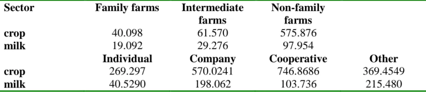
Table 4. The mean size of farms according to farm organisation in Bulgarian crop and milk production (in hectares for crop farms; in livestock units for milk farms) (first typology = Hill typology; second typology = FADN typology)

Sector

Family farms

Intermediate

farms

Non-family

farms

crop

40.098

61.570

575.876

milk

19.092

29.276

97.954

Individual

Company

Cooperative

Other

crop

269.297

570.0241

746.8686

369.4549

milk

40.5290

198.062

103.736

215.480

Source: own calculations based on FADN database

Table 5. The mean size of farms according to farm organisation in Estonian crop and milk production (in hectares for crop farms; in livestock units for milk farms) (first typology = Hill typology; second typology = FADN typology)

Sector

Family farms

Intermediate farms

Non-family farms

crop

133.650

194.305

413.125

milk

29.788

45.820

243.99

Individual

Company

milk

42.407

342.938

Source: own calculations based on FADN database

Table 6. The mean size of farms according to farm organisation in Hungarian crop and milk production (in hectares for crop farms; in livestock units for milk farms) (first typology = Hill typology; second typology = FADN typology)

Sector

Family farms

Intermediate farms

Non-family farms

crop

79.108

132.390

540.840

milk

26.706

48.938

428.248

Individual

Company

Cooperative

crop

129.634

687.664

822.640

milk

79.1502

647.997

579.660

Source: own calculations based on FADN database

Our calculations confirm the hypothesis that individual farms are small farms. The results in tables 4-6 show that individual farms are smaller than companies and cooperatives for all countries and products. However, the size of family farms is much lower than the one for individual farms on average. The figures suggest a linear relationship between the size and Hill type farms from family farms to non-family farms.

In sum, we conclude that the conceptual farm typology and official farm classification system does not correspond to each other. Consequently, the exclusive use of any farm classification may have serious consequences on empirical research especially in terms of policy implications.

3

Methodology

There are two main approaches developed over time, for analysing technical efficiency in agriculture. (1) The construction of a nonparametric piecewise linear frontier using linear programming method known as data envelopment analysis (DEA); (2) the estimation of a parametric production function using stochastic frontier analysis (SFA). In addition to these two widely used methods, we also employ the operational competitiveness rating (OCRA) method which is a relative performance measurement approach based on a non-parametric model. We briefly review all of these methodologies.

3.1 The OCRA method

2

Parkan (1991) developed the OCRA method, which is still not so popular compared to the DEA or SFA approaches. Recently Parkan and Wu (2000) provide an interesting comparison on three different non-parametric approaches. Suppose that we want to compare the operational performances of K Decision Making Units (DMUs) that consume resources in M categories (the input-side) and generate revenues in H categories (the output-side). A DMU may represent the operation of an operating entity in a given year. Let vectors uk = (uk1; . . . ; ukM) and vk = (vk1; . . . ; vkH) represent the kth DMU's input values (costs) and output values (revenues), respectively. We assume that there exists a convex, at least once differentiable and increasing, function E of (u, -v), whose value gauges the relative performance of a DMU's operation in converting the inputs of resources into the outputs of products. The kth DMU is assigned a rating to gauge its performance so that among all DMUs whose performance is inferior to the kth DMU, the kth DMU's function value, Ek = E(uk, -vk) is the smallest, k = 1; . . . ; K. This can be expressed as the following convex programming problem for k = 1; . . . ; K: Ek= E(uk, - vk) = v u,

min

{E(uk, - vk): um ≥ ukm, m = 1,...,M; vh ≤ vkh, h = 1,...,H; u, v ≥ 0} (1)

Ek in Eq. (1) gauges the relative operational performance rating of the kth DMU. It has been shown in

several studies that the saddle-point theorem of mathematical programming can be used to obtain the following optimality conditions for Eq. (1):

Ek - En -

∑

= M m 1 αkm(unm - ukm)/ukm +

∑

= H h 1 βkh(vnh - vkh)/vkh≥ 0, k, n = 1,...,K, (2)

2

where the multipliers αkm and βkh are such that αkm ≥ akm > 0, βkh≥ bkh > 0, k = 1,...,K, m = 1,...,M and

h = 1,...,H. The positive constants akm and bkh are called calibration constants and they reflect the

relative importance that the kth DMU assigns to the mth resource category and the hth revenue category, respectively. If every DMU assigns the same relative importance to a resource consumption or revenue generation category, that is, if for k = 1,...,K, akm=am, m = 1,...,M, and bkh=bh, h = 1,...,H,

then the kth DMU's performance rating, Ek , can be obtained by the following simple procedure:

(a)

Compute the kth DMU's resource consumption performance rating C

k

by computing

first its resource consumption performance rating with respect to the mth input

category

Ckm = am[ukm - K

i

min

=1,..., {uim}] / i

min

=1,...,K{uim}, m = 1,...,M (3)

and then linearly scaling their sum by

Ck =

∑

= M m 1 Ckm - K n

min

=1,..., {

∑

₌ M m 1 Cnm} =

∑

= M m 1 am[ukm - i

min

{uim}] / i

min

{uim} - n

min

{

∑

= M m 1 am[ukm - i

min

{uim}] / i

min

{uim}} (4)

so that a value of zero is obtained for

K i

min

=1,..., {Ck}

(b) Compute the kth DMU's revenue generation performance rating Rk by first computing its

revenue generation performance rating with respect to the hth output category by

Rkh = bh[ K i

max

=1,..., {vih} - vkh] / K i

min

=1,..., {vih}, h = 1,...,H (5)

and then linearly scaling their sum by

Rk =

∑

= H h 1 Rkh - K n

min

=1,..., {

∑

₌ H h 1 Rnh} =

∑

= H h 1 bh[ i

max

{vih} - vkh] / i

min

{vih} - n

min

{

∑

= H h 1 bh[ i

max

{vih} - vnh] / i

min

{vih}} (6)

so that a value of zero is obtained for

K i

min

=1,..., {Rk}.

(c) Compute the kth DMU's overall operational performance rating by linearly scaling the weighted sum of Ck and Rk by

Ek = wcCk + wrRk - K

= wc

∑

= M m 1 am[ukm - i

min

{uim}] / i

min

{uim} + wr

∑

= H h 1 bh[ i

max

{vih} - vkh] / i

min

{vih} - n

min

{ wc

∑

= M m 1 am[ukm - i

min

{uim}] / i

min

{uim} + wr

∑

= H h 1 bh[ i

max

{vih} - vnh] / i

min

{vih}} (7)

so that a value of zero is obtained for

K i

min

=1,...,

{Ek}. In Eq. (7), wc and wr are calibration

constants reflecting the relative importance of the input and output categories.

OCRA's assessment criterion is such that the smaller the rating Ek , the better the kth DMU's relative

operational performance. The DMU with the best operational performance receives an operational performance rating of zero.

Normalized calibration constants

The calibration constants of the models presented in the previous section represent the relative importance of the input and output categories they are associated with. Operational performance ratings obtained using different calibration constants would be comparable if they are normalized so that their sum is a constant. Thus, we make sure that

∑

= M m 1 am =

∑

= H h 1 bh = wc + wr = 1 (8)

We use an intuitive procedure to obtain sensible initial values for the calibration constants. In our approach, an input category is assigned a calibration constant value that is in proportion to the costs incurred in that category. A revenue category is assigned a calibration constant value in a similar manner. Since the values of the calibration constants should reflect the relative importance of the various input and output categories, an input category whose costs are higher than those of another category is assigned a relatively larger cost calibration. This approach has some similarity to the entropy method of assigning weights to attributes in the context of multiple criteria decision making (MCDM) where an attribute with relatively large variation receives a larger weight. The procedure consists of the following steps:

(a) Define wc and wr as the average total cost and revenue shares, respectively, which are

computed by wc =

∑

= K k 1 [

∑

= M m 1 ukm / (

∑

= M m 1 ukm +

∑

= H h 1 vkh ) ] / K,

wr =

∑

= K k 1 [

∑

= H h 1 vkh / (

∑

= M m 1 ukm +

∑

= H h 1 vkh ) ] / K = 1- wc (9)

(b) Compute the calibration constants am and bh by

am =

∑

= K k 1 [ ukm /

∑

= M m 1 ukm ] / K, m = 1,...,M, bh =

∑

= K k 1 [vkh /

∑

= H h 1 vkh ] / K, h = 1,...,H (10)

The first expression in Eq. (10) defines am as the average cost share of the mth cost category and the

second expression defines bh as the average revenue share of the hth revenue category. Eqs. (9) and

(10) satisfy Eq. (8).

It should be noted that, partly due to the fact that the calibration constants in Eqs. (9) and (10) are scale dependent, the OCRA procedure as described in Eqs. (3) - (7) may have the rank reversal problem. The rank-reversal problem relates to the change of the performance rank order of the DMUs when one or more DMUs are removed from the list and is, in fact, associated with many MCDM and performance measurement techniques. For example, the Analytic Hierarchy Process (AHP), a popular MCDM method, has a serious rank reversal problem that has been the topic of many discussions. Even in the IMD's simple additive weighting approach, where a standard deviation transformation is employed to convert the original data into a comparable scale for each criterion, there may be rank reversals when some of the observations are removed from or new ones are added to the competitiveness analysis. OCRA's rank reversal problem is less serious than AHP's. For example, for a given set of calibration constants, the rank order of the DMUs' performance ratings obtained by the OCRA procedure in Eqs. (3) - (7) will remain unchanged if DMUs that do not contain the maximum and minimum cost/revenue values for all resource and revenue categories are removed. OCRA's rank reversal problem has a simple solution: introduce one positive and one negative benchmark DMU that outperforms every DMU and is outperformed by every DMU in all resource and revenue categories, respectively.

3.2 The Stochastic Frontier Analysis method

Within the parametric approaches, the Stochastic Frontier Analysis, (SFA) is commonly used. Aigner

at al. (1977) and Meeusen and Van den Broeck (1977) have simultaneously yet independently

developed the use of SFA in efficiency analysis.

The main idea is to decompose the error term of the production function into two components, one pure random term (vi) accounting for measurement errors and effects that can not be influenced by the

firm such as weather, trade issues, access to materials, and a non-negative one (ui) measuring the

technical inefficiency, i.e. the systematic departures from the frontier:

)

exp(

)

(

i i i i

f

x

v

u

Y

=

−

or, equivalently: (11)

)

)

ln(

Y

i

=

β

x

i

+

v

i

−

u

i

where Yi is the output of the i th

firm, xi is a (k+1) vector of inputs used in the production, f(·) is the

production function, ui and vi the error terms explained above, and finally, β a (k+1) the column vector

of parameters to be estimated. The output oriented technical efficiency (TE) is actually the ratio between the observed output of firm i and the distance to the frontier, i.e. to the maximum possible output using the same input mix xi.

Arithmetically, technical efficiency is equivalent with:

) exp( ) exp( ) exp( * i i i i i i i i i u v x u v x Y Y TE = − + − + = =

β

β

,

0

≤

TE

i

≤

1

. (12)

Contrary to the non-parametric DEA approach, where all technical efficiency scores are located on, or below the efficient frontier (see below), in SFA they are allowed to be above the frontier, if the random error v is larger than the non-negative u.

Applying SFA methods requires distributional and functional form assumptions. First, because only the wi = vi - ui error term can be observed, one needs to have specific assumptions about the

distribution of the composing error terms. The random term vi, is usually assumed to be identically and

independently distributed drawn from the normal distribution, N(0,

σ

v2), independent of ui. There are

a number of possible assumptions regarding the distribution of the non-negative error term ui

associated with technical inefficiency. However most often it is considered to be identically distributed as a half normal random variable, N (0,

σ

u2)

+ _{or a normal variable truncated from below zero,}

) , ( u2 N+

µ

σ

_.

Second, being a parametric approach, we need to specify the underlying functional form of the Data Generating Process, DGP. There are a number of possible functional form specifications available, however most studies employ either Cobb-Douglas (CD):

∏

= = K k ik i k x e x f 1 0 ) ( β β (13) or TRANSLOG (TL) specification:

∑∑

∑

= = =

+

=

K k K j jk ik kj K k ik k i

x

x

x

x

f

1 1 1

ln

ln

2

1

ln

)

(

ln

β

β

. (14)

Because the two models are nested, it is possible to test the correct functional form by a Likelihood Ratio, LR test. The TL is a more flexible functional form, whilst the CD restricts the elasticities of substitution to 1. The model could be estimated either with Corrected Ordinary Least Squares, COLS or Maximum Likelihood, ML. With the availability of computer software, the estimation by ML became less computationally demanding, and the ML estimator was found to be significantly better than COLS (Coelli et al.,2005).

With panel data, TE can be chosen to be time invariant, or to vary systematically with time. To incorporate time effects, Battese and Coelli (1992) define the non-negative error term as exponential function of time:

i

it

t

T

u

u

=

exp[(

−

η

(

−

)]

(15)

where t is the actual period, T the final period, and η a parameter to be estimated. TE either increases (η>0), decreases (η<0) or it is constant over time, i.e. invariant (η=0). LR tests can be applied to test the inclusion of time in the model. Since TE is allowed to vary, the question arises what determines the changes of TE scores. Early studies applied a two-stage estimation procedure, first determining the inefficiency scores, and then, in a second stage regressing TE scores upon a number of firm specific variables assumed to explain changes in inefficiency scores. Some authors however showed that conflicting assumptions are needed for the two different estimation stages. In the first stage, the error terms representing inefficiency effects are assumed to be independently and identically distributed, whilst in the second stage they are assumed to be function of firm specific variables explaining inefficiency, i.e. they are not independently distributed (Curtiss, 2002). Battese and Coelli (1995) proposed a one stage procedure where firm specific variables are used to explain the predicted inefficiencies within the SFA model. The explanatory variables are related to the firm specific mean μ of the non-negative error term ui:

∑

= j ij j i

δ

z

µ

(16) where μi is the i th

firm-specific mean of the non-negative error term; δj are parameters to be estimated;

zij are ith firm-specific explanatory variables.

Using cross-section or panel data may often lead to heteroscedasticity in the residuals. With heteroscedastic residuals, OLS estimates remain unbiased but no longer efficient. In frontier models however, the consequences of heteroscedasticity are much more severe, as the frontier changes when the dispersion increases. Caudill et al. (1995) introduced a model which incorporates heteroscedasticity into the estimation. That is done by modelling the relationship between the variables responsible for heteroscedasticity and the distribution parameter σu:

) exp(

∑

= j j ij ui x

ρ

σ

(17)

where xij are the jth input of the ith farm, the input assumed to be responsible for heteroscedasticity, and

ρj a parameter to be estimated.

Within SFA approach it is possible to test whether any form of stochastic frontier production function is required or the OLS estimation is appropriate using a LR test. Using the parameterisation of Battese

and Cora (1977), define γ, the share of deviation from the frontier that is due to inefficiency:

2 2 2 u v u

σ

σ

σ

γ

+

=

(18)

where σ2v is the variance of the v and σ 2

u the variance of the u error term.

It should be noted however, that the test statistic has a ‘mixed’ chi square distribution, with critical values tabulated in Kodde and Palm (1996).

3.3 The Data Envelopment Analysis method

DEA was introduced by Charnes et al. (1978) based on the seminal work of Farrell (1957). We can divide the DEA method into two main groups: constant return to scale and variable return to scale models.

3.3.1 The Constant Return to Scale (CRS) model

In the model presented below Constant Return to Scale (CRS) and input orientation are assumed. This model yields an objective evaluation of overall technical efficiency (TE) and estimates the amounts of the identified inefficiencies.

The data relate to

𝐾

inputs and

𝑀

outputs on each of 𝑁 firms. For the ith firm, these are represented by the vectors

𝑥

_𝑗 and

𝑦

_𝑗. The data of all

𝑁

firms are represented by

𝐾𝑋 × 𝑁

input matrix (X) and by

𝑀𝑌 × 𝑁

output matrix

(𝑌

). The purpose of DEA is to construct a non-parametric envelopment frontier over the data points such that all observed points lie on or below the production frontier. The frontier is therefore constructed with the best performing farms of the sample.

The DEA model involves optimising a scoring function (H), defined as the ratio of the weighted sum of outputs and the weighted sum of inputs. This function is optimised, subject to the condition that the value of the objective function achieved can not be greater than one, implying that efficient units will have a score of one. For each ith firm, the linear problem is the following:

max

_𝑢,𝑣

𝐻 = (u′𝑦

𝑖

/v′𝑥

𝑖

)

𝑠𝑡 (u′𝑦

𝑗

/v′𝑥

𝑗

) ≤ 1, 𝑗 = 1,2, … , 𝑁

u,v ≥ 0

(19)

where

u′𝑦

_𝑖

/v′𝑥

_𝑖, is the scoring function (

u

is an

𝑀 × 1

vector of output weights and

v

is an

𝐾 × 1

vector of input weights). The goal is to find values for u and v that maximise the efficiency score of the ith firm subject to the constraint that all the efficiency measures must be less than or equal to one.

The ratio formulation of the model has infinite number of solutions and to avoid this problem it is necessary to impose the constraint:

𝑣𝑥

𝑖

= 1

Then, the maximization becomes

max

_𝜇,𝑣

(𝜇′𝑦

𝑖

)

𝑠𝑡 𝑣′𝑥

𝑖

= 1

𝜇′𝑦

𝑗

− 𝑣′𝑥

𝑗

≤ 1, 𝑗 = 1,2, … , 𝑁

𝜇, 𝑣 ≥ 0

(20)

This transformation of

u

and

v

in

𝜇

and

𝑣

, is identified with multiplier form of the DEA linear programming problem.

Introducing the duality in linear programming, one can derive an equivalent envelopment form of this problem:

TE

crs

= min

θ,𝜆

𝜃

𝑠𝑡 − 𝑦

𝑖

+ 𝑌𝜆 ≥ 0 (1)

𝜃𝑥

𝑖

− 𝑋𝜆 ≥ 0 (2)

𝜆 ≥ 0

where

𝜃

is a scalar that represents the minimum level to which the use of inputs can be reduced without altering the output level. So, the scalar

𝜃

provides the value of the global technical efficiency score for the ith firm. Indeed, following the Farrell’s definition (1957),

𝜃

will satisfy the condition of less than or equal to 1: if it is equal to one, the firm is considered technically efficient (it is a point on the frontier). It means also that the use of all inputs cannot be reduced at the same time without altering technical efficiency, although a variation in the use of one of them may improve efficiency. If the index is less than one there is some degree of technical inefficiency (firms are below the frontier).

𝜆

is a

𝑁 × 1

vector of constants that represents the weights to be used as multipliers for the input levels of a reference production unit to indicate the input levels that an inefficient unit should aim at in order to achieve efficiency.

It’s important to underline that for each firm we must find a value of

𝜃

, and therefore the linear programming problem must be solved

𝑁

times, one for each firm in the sample.

3.3.2 The Variable Return to Scale (VRS) model

The CRS DEA model is appropriate only when the farm is operating at an optimal scale. The previous model thus permits to obtain a measure of global technical efficiency that does not allow variations in returns to scale. The VRS model is an extension of the CRS DEA model, introduced to take into

account some factors such as imperfect competition, constraints, on finance, etc., that may cause the firm to be not operating at an optimal level in practice. This model distinguishes between pure technical efficiency (calculated with the VRS model) and scale efficiency (SE), identifying whether increasing, decreasing or constant returns to scale possibilities are present for further exploitations.

As a consequence, the CRS linear model presented above changes by adding a further convexity constraint:

𝑁1

′

_{𝜆 = 1}

₍₂₁₎

Hence, the envelopment form of the input oriented VRS DEA model is specified as

TE

vrs

= min

θ,𝜆

𝜃

𝑠𝑡 − 𝑦

𝑖

+ 𝑌𝜆 ≥ 0

𝜃𝑥

𝑖

− 𝑋𝜆 ≥ 0

𝑁1

′

_{𝜆 = 1}

𝜆 ≥ 0

where

𝑁1

is a

𝑁 × 1

vectors of ones.

θ is the input technical efficiency score, having a value 0 < θ ≤ 1. As the previous case, if the θ value

is equal to one, the firm is on the frontier; the vector λ is an

𝑁 × 1

vector of weights which defines the linear combinations of the peers of the ith firm.

Because the VRS DEA model is more flexible and envelops the data in a tighter way than the CRS DEA model, the VRS technical efficiency score is equal to or greater than the CRS score also called the overall technical efficiency score. This relationship can be used to measure the scale efficiency of the firms defined as the ratio of the TE score obtained under CRS (the total technical efficiency score) to the TE score obtained under VRS (the pure technical efficiency score):

𝑆𝐸 =

𝑇𝐸𝑐𝑟𝑠

𝑇𝐸𝑣𝑟𝑠 (22)

SE = 1 implies scale efficiency or the presence of CRS, while SE < 1 indicates scale inefficiency that can be due to the existence of either increasing or decreasing returns to scale. This may be determined by calculating an additional DEA problem with non-increasing returns to scale (NIRS) imposed. The previous VRS DEA model may be changed replacing the

𝑁1

′

𝜆 = 1

restriction with

𝑁1

′

𝜆 ≤ 1

. IF the NIRS TE score is different to the VRS TE score, it indicates that increasing returns to scale exist for the firm. If they are equal, then decreasing returns to scale apply.

3.4 Second stage regression

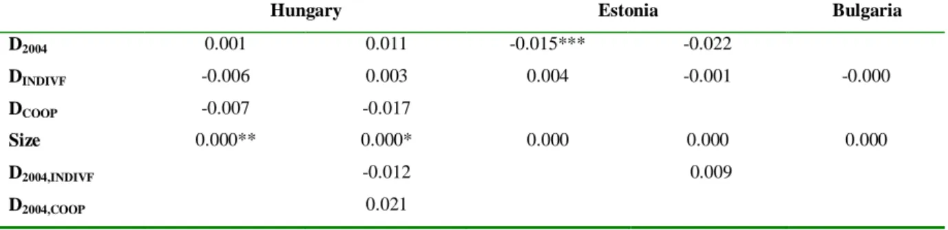
Efficiency scores obtained with the methods discussed in the previous section (SFA, DEA and OCRA), are used in second stage panel estimations in order to evaluate similarities and differences

between farms in New Member States, with special emphasis on farm type. Depending on the definition of farm type (see section 2), the following two equations (Eqs. (23) and (24)) are estimated:

(23)

where:

- TE are the technical efficiency scores estimated with SFA, DEA and OCRA respectively, - D2004 is a dummy variable representing EU accession effects (except for Bulgaria),

- Dindiv is a dummy variable that takes the value of 1 if the farm is individual farm and 0 otherwise, - Dcoop is a dummy variable that takes the value of 1 if the farm is a cooperative, and 0 otherwise, - Size is a variable measuring the farm size expressed in European Size Units (SIZE in the FADN

database),

- D2004Indiv is the interaction term between the EU accession dummy and family farm dummy, - D2004Coop is the interaction term between the EU accession dummy and cooperative farm dummy, - D2004Size is the interaction term between the EU accession dummy and farm size variable.

(24)

where:

- TE are the technical efficiency scores estimated with SFA, DEA and OCRA respectively, - D2004 is a dummy variable representing EU accession effects (except for Bulgaria),

- Dfamilyf is a dummy variable that takes the value of 1 if the farm is family farm according to Hill classification (family labour>95%), and 0 otherwise,

- Dintermf is a dummy variable that takes the value of 1 if the farm is an intermediate farm, according to Hill classification (family labour>50%) and 0 otherwise,

- Size is a variable measuring the farm size expressed in European Size Units (SIZE in the FADN database),

- D2004familyf is the interaction term between the EU accession dummy and family farm dummy, - D2004intermf is the interaction term between the EU accession dummy and intermediate farm

dummy,

- D2004Size is the interaction term between the EU accession dummy and farm size variable.

Due to the time invariant nature of farm type and legal type variables we apply random effect panel models. Following recommendation by Baltagi (2008) to deal with unbalanced nature of our dataset we apply ANOVA estimators, however unbalancedness of our data is not severe.

Size D b coop D b indiv D b Size coop D indiv D D TE 2004 1 , 2004 3 , 2004 2 1 3 2 2004 1

δ

β

β

δ

β

β

β

α

+ + + + + + + + =

Size

D

b

ermf

D

b

familiyf

D

b

Size

ermf

D

familyf

D

D

TE

2004

1

int

,

2004

3

,

2004

2

1

int

3

2

2004

1

δ

β

β

δ

β

β

β

α

+

+

+

+

+

+

+

+

=

4

The pattern of farm performance in

Bulgaria, Estonia and Hungary

Our approaches to measure farm performance assume that technology is the same for each producer, thus we need to ensure relatively homogenous samples. Consequently we moved to specific product groups instead of using the whole sample of the national FADN database. To analyse the farm performance we focus on two main product groups: field crops and dairy. The rationale of this selection is based on the significance of these products in our sample countries’ agriculture. Specific efficient frontiers were computed for field crop farms on one hand, and dairy farms on the other hand.

We are interested in three specific questions. First, what is the evolution of the farm performance over time in the analysed countries? Second, is the general pattern of farm performance similar using different estimation methods? Finally, does the pattern of farm performance differ across farm types using different typologies (official FADN versus Hill)?

The next section graphically presents the yearly mean technical efficiency scores for specialised field crop and dairy farms in the three NMS (Bulgaria, Estonia and Hungary). Country, sector and farm typology specific mean technical efficiency scores and their Bartlett’s equality tests are computed and presented in the tables under the graphs.

4.1 Mean technical efficiency scores

To present our results we face the following difficulties. Whilst the DEA and SFA scores range between zero and one, similar or predetermined intervals do not exist for the OCRA score. Thus, we should apply various scales for DEA/SFA and OCRA, respectively. So, in the following figures, the left vertical axis shows the DEA/SFA scores, the right vertical axis presents the OCRA scores. Due to this scaling issue it should be noted that the following figures have an illustrative purposes.

The legal farm type classification, within the FADN database, consists of individual, company and cooperative farms (with exception of Estonia, where there are no cooperatives). The Hill-type farm classification consists of family, intermediate and non-family farm types. The null hypothesis of the Bartlett’s mean equality test is that computed farm type specific means are equal. The test statistics in the following tables are levels of significance (probabilities of committing Type I error).

Figure 1 shows rather contradictory results for Hungarian crop producers, namely each indicator suggest a different trend, but last two years all measures shows an improvement in farm performance.

Figure 1. Mean technical efficiency scores obtained with the three methods – field crops, Hungary (left axis: measures of SFA and DEA; right axis: measures for OCRA)

The means of the performance indicators differ by legal type and farm type, except for the SFA method. The general ranking of farm types and legal forms are independent from the methods. The companies perform the best followed by cooperative and individual farms (Table 7). Regarding the Hill-type classification we can observe that non-family farms are better than intermediate farms, and family farms are the worst (Table 8).

Table 7. Efficiency means and mean equality tests according to legal type – field crops, Hungary individual company cooperative Bartlett's test

SFA_crop 0.744 0.7531 0.743 0.227

DEA_crop 0.457 0.518 0.513 0.000

OCRA crop 504.453 509.512 505.025 0.000

Source: own calculations based on FADN database

Table 8. Efficiency means and mean equality tests according to Hill classification – field crops, Hungary

family farms intermediate farms

non family farms Bartlett's test

SFA_crop 0.741 0.748 0.750 0.001

DEA_crop 0.448 0.448 0.510 0.000

OCRA crop 502.894 504.031 509.179 0.000

Source: own calculations based on FADN database

470 480 490 500 510 520 530 0 0,1 0,2 0,3 0,4 0,5 0,6 0,7 0,8 0,9 2001 2002 2003 2004 2005 2006 2007 2008

The average performance for Hungarian dairy farmers is rather stable after 2002 with DEA and SFA scores, whilst OCRA presents a declining trend with a sudden increase in 2008. But all three methods suggest an improvement for the last year (Figure 2).

Figure 2. Mean technical efficiency scores obtained with the three methods – dairy, Hungary

(left axis: measures of SFA and DEA; right axis: measures for OCRA)

Similarly to the crop farms, the average performance of dairy farms differ significantly by legal type and farm type, except for the DEA method. The ranking of farm types and legal forms show similar patterns as for crop farms. The companies display the best performance followed by cooperative and individual farms, except for SFA (Table 9). Our results imply that according to the Hill-classification non-family farms are on the top followed by intermediate farms, and family farms (Table 10).

Table 9. Efficiency means and mean equality tests according to legal type – dairy, Hungary individual company cooperative Bartlett's test

SFA_dairy 0.857 0.887 0.889 0.000

DEA_dairy 0.648 0.769 0.641 0.622

OCRA dairy 378.06 445.320 403.294 0.000

Source: own calculations based on FADN database

Table 10. Efficiency means and mean equality tests according to Hill classification – dairy, Hungary family farms intermediate

farms non family farms Bartlett's test SFA_dairy 0.851 0.860 0.877 0.000 DEA_dairy 0.6157 0.648 0.720 0.386 OCRA dairy 369.0480 372.1820 418.291 0.000

Source: own calculations based on FADN database

320 340 360 380 400 420 440 0 0,1 0,2 0,3 0,4 0,5 0,6 0,7 0,8 0,9 1 2001 2002 2003 2004 2005 2006 2007 2008

Estonian estimations suggest more consistent results. All of the three methods show a fairly stable pattern with a small fluctuation for Estonian crop producers (Figure 3). We can not observe any significant changes after the EU accession.

Figure 3. Mean technical efficiency scores obtained with the three methods – field crops, Estonia (left axis: measures of SFA and DEA; right axis: measures for OCRA)

Calculations confirm that there is a significant difference in farm performance between legal types for all performance indicators considered. The companies perform better than individual farms (Table 11). Interestingly, the differences between score means following the Hill-classification are not significant except for OCRA measures, where non-family farms report the best results followed by intermediate farms and individual farms (Table 12).

Table 11. Efficiency means and mean equality tests according to legal type – field crops, Estonia

individual company Bartlett's test

SFA_crop 0.801 0.803 0.050

DEA_crop 0.613 0.693 0.081

OCRA crop 47.279 47.425 0.000

Source: own calculations based on FADN database

Table 12. Efficiency means and mean equality tests according to Hill classification – field crops, Estonia

family farms intermediate farms non family farms Bartlett's test SFA_crop 0.794 0.815 0.804 0.359 DEA_crop 0.571 0.669 0.688 0.210 OCRA crop 44.528 48.672 51.621 0.000

Source: own calculations based on FADN database

0 10 20 30 40 50 60 0 0,1 0,2 0,3 0,4 0,5 0,6 0,7 0,8 0,9 2001 2002 2003 2004 2005 2006 2007 2008

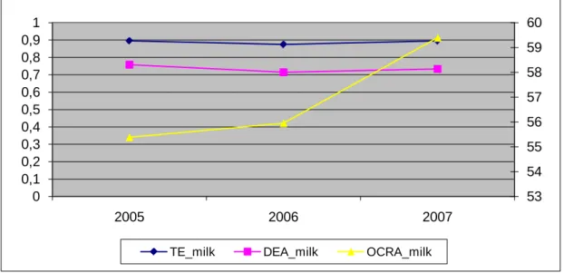
Estonian dairy farms show a bit different picture. The DEA and SFA scores suggest a relatively constant pattern, whilst OCRA calculations present an increasing trend with some fluctuations (Figure 4).

Figure 4. Mean technical efficiency scores obtained with the three methods – dairy, Estonia (left axis: measures of SFA and DEA; right axis: measures for OCRA)

Estimations confirm that there is a significant difference in farm performance between legal types for Estonian dairy farms, except for DEA (Table 13). Surprisingly, the SFA and OCRA scores yield opposite results, with SFA suggesting no superiority of individual farms, whilst OCRA suggests advantages for companies. The calculations by farm type according to the Hill-classification produce more unambiguous results. DEA and OCRA measures shows that non-family farms report the best results followed by intermediates farms and individual farms (Table 14).

Table 13. Efficiency means and mean equality tests according to legal type – dairy, Estonia

individual company Bartlett's test

SFA_dairy 0.888 0.886 0.013

DEA_dairy 0.710 0.794 0.133

OCRA dairy 54.355 89.345 0.000

Source: own calculations based on FADN database

Table 14. Efficiency means and mean equality tests according to Hill classification – dairy, Estonia family farms intermediate

farms non family farms Bartlett's test SFA_dairy 0.886 0.890 0.889 0.656 DEA_dairy 0.695 0.725 0.773 0.005 OCRA dairy 52.643 55.016 77.991 0.000

Source: own calculations based on FADN database

50 52 54 56 58 60 62 64 66 0 0,1 0,2 0,3 0,4 0,5 0,6 0,7 0,8 0,9 1 2001 2002 2003 2004 2005 2006 2007 2008

For Bulgaria we only have a three years period. SFA and DEA scores show a slightly declining trend for crop farmers, whilst OCRA present a considerable fluctuation (Figure 5).

Figure 5. Mean technical efficiency scores obtained with the three methods – field crops, Bulgaria (left axis: measures of SFA and DEA; right axis: measures for OCRA)

Calculations present clear evidence that there is a significant difference in farm performance between legal types for Bulgarian crop producers, except for SFA measures. The ranking is the following: best performing are cooperatives, followed by companies and individual farms (Table 15). Estimations according to the Hill-classification are consistent in terms of ranking: non-family farms report the best results followed by intermediate farms and individual farms (Table 16).

Table 15. Efficiency means and mean equality tests according to legal type – field crops, Bulgaria individual company cooperative other Bartlett's

test

SFA_crop 0.736 0.717 0.749 0.726 0.422

DEA_crop 0.556 0.584 0.621 0.506 0.027

OCRA crop 4812.557 5103.285 5136.358 4882.222 0.000

Source: own calculations based on FADN database

Table 16. Efficiency means and mean equality tests according to Hill classification – field crops, Bulgaria

family farms intermediate farms non family farms Bartlett's test SFA_crop 0.717 0.730 0.744 0.003 DEA_crop 0.445 0.540 0.619 0.267 OCRA crop 4640.592 4656.45 5035.721 0.000

Source: own calculations based on FADN database

4600 4650 4700 4750 4800 4850 4900 4950 5000 5050 0 0,1 0,2 0,3 0,4 0,5 0,6 0,7 0,8 0,9 2005 2006 2007

Finally, we turn to the Bulgarian dairy farmers. The DEA and SFA display a stable pattern, the OCRA shows a growing trend (Figure 6).

Figure 6. Mean technical efficiency scores obtained with the three methods – dairy, Bulgaria (left axis: measures of SFA and DEA; right axis: measures for OCRA)

Similarly to the crop farms, the mean performances of dairy farms differ significantly by FADN legal type and by Hill farm type, except for the DEA method. The ranking of farm types however reports contradictory results. SFA suggests the following order: best performing are individual farm, followed by company and cooperative, whilst OCRA shows: companies as the best performers, followed by cooperatives and individual farms (Table 17). Results are also ambiguous when Hill farm types are considered. Estimations based on SFA imply that intermediate farms are on the top followed by non-family farms and non-family farms, whilst OCRA favours to non-non-family farms against intermediate and family farms (Table 18).

Table 17. Efficiency means and mean equality tests according to legal type – dairy, Bulgaria individual company cooperative other Bartlett's

test

SFA_dairy 0.863 0.832 0.831 0.821 0.000

DEA_dairy 0.580 0.828 0.781 0.639

OCRA dairy 96.643 244.317 218.69 345.927 0.000

Source: own calculations based on FADN database

Table 18. Efficiency means and mean equality tests according to Hill classification – dairy, Bulgaria family farms intermediate

farms non family farms Bartlett's test SFA_dairy 0.850 0.865 0.860 0.000 DEA_dairy 0.507 0.583 0.650 0.462 OCRA dairy 78.380 84.859 162.500 0.000

Source: own calculations based on FADN database

53 54 55 56 57 58 59 60 0 0,1 0,2 0,3 0,4 0,5 0,6 0,7 0,8 0,9 1 2005 2006 2007

In sum, our calculations reject the ability of three different approaches to provide a consistent picture on farm performance on selected countries. But the majority of results confirm that individual and family farms perform worse than the corporate farm organisation, irrespective of the method, product group and country.