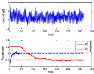
Parameter estimation of a 3-level quantum system with a single population measurement

autobiographique, il convient d’entendre un récit linéaire, on commence par une introduction classique qui narre le point de vue de départ de l’histoire, pour ensuite revenir vers

In the study of open quantum systems modeled by a unitary evolution of a bipartite Hilbert space, we address the question of which parts of the environment can be said to have

Several challenges remain to be overcome on the way to a full understanding of nonequilibrium quantum thermo- dynamics in the resonant-level model: Beyond the wide- band

Abstract. This supports the arguments that the long range order in the ground state is reached by a spontaneous symmetry breaking, just as in the classical case...

( ﺫﻴﻔﻨﺘ ﺭﺎﻁﺇ ﻲﻓ ﺔﻠﻴﺴﻭﻟﺍ ﻩﺫﻫ لﺎﻤﻌﺘﺴﺇ ﻯﺩﻤ ﻰﻠﻋ ﻑﻭﻗﻭﻟﺍ ﻱﺭﻭﺭﻀﻟﺍ ﻥﻤ ﻪﻨﺈﻓ ﻲﻟﺎﺘﻟﺎﺒﻭ ﻕﻭﺴﻟﺍ ﺩﺎﺼﺘﻗﺍ ﻯﻭﺤﻨ لﺎﻘﺘﻨﻹﺍ ﻭ ﺔﻴﺩﺎﺼﺘﻗﻹﺍ ﺕﺎﺤﻼﺼﻹﺍ. ﺔﺴﺍﺭﺩﻟﺍ ﺭﺎﻁﺍ ﺩﻴﺩﺤﺘ :

Non-integrable quantum phase in the evolution of a spin-1 system : a physical consequence of the non-trivial topology of the quantum state-space... Non-integrable quantum phase in

To get the highest homodyne efficiency, the phases of the quantum field and local oscillator have to be matched (see Section III). Assuming the phase θ LO of the local oscillator to

L’archive ouverte pluridisciplinaire HAL, est destinée au dépôt et à la diffusion de documents scientifiques de niveau recherche, publiés ou non, émanant des