HAL Id: hal-00865671
https://hal.sorbonne-universite.fr/hal-00865671
Submitted on 24 Sep 2013
HAL is a multi-disciplinary open access
archive for the deposit and dissemination of
sci-entific research documents, whether they are
pub-lished or not. The documents may come from
teaching and research institutions in France or
abroad, or from public or private research centers.
L’archive ouverte pluridisciplinaire HAL, est
destinée au dépôt et à la diffusion de documents
scientifiques de niveau recherche, publiés ou non,
émanant des établissements d’enseignement et de
recherche français ou étrangers, des laboratoires
publics ou privés.
Pressure Boundary Conditions for Blood Flows
Kirill Gostaf, Olivier Pironneau
To cite this version:
AIMS’ Journals
Volume X, Number 0X, XX 200X pp. X–XX
PRESSURE BOUNDARY CONDITIONS FOR BLOOD FLOWS
Kirill Pichon Gostaf
Department of Mathematics, Simon Fraser University, Burnaby V5A 1S6, BC, Canada Olivier Pironneau
LJLL-UPMC, Boite 187, Place Jussieu, 75252 PARIS cedex 5, France
Abstract. Simulations of blood flows in arteries require numerical solutions of fluid-structure interactions involving Navier-Stokes equations coupled with large displacement visco-elasticity for the vessels.
Among the various simplifications which have been proposed, the surface pressure model leads to a hierarchy of simpler models including one which involves only the pressure. The model exhibits fundamental frequencies which can be computed and compared with the pulse. Yet unconditionally stable time discretizations can be constructed by combining implicit time schemes with Galerkin-characteristic discretization of the convection terms in the Navier-Stokes equations. Such problems with prescribed pressure on the walls will be shown to be efficient and accurate as an approximation of the full fluid structure interaction problem.
1. Introduction. Computational Hemodynamics is a major research field with many applications to the human blood circulatory system – especially for heart diseases and aneurysms – leading to diagnostic tools and simulations of chirurgical
treatments like stents (see [34]) and by-passes (see Thiriet[35]).
Since the pioneering work of Peskin [27] impressive progress has been made both
on the methodological side, namely the treatment of moving walls, cardiac muscles etc, and on the numerical side for efficient and stable discretizations of these fluid
structure interaction problems. Some are presented in [13]; mostly with methods
on fixed domains after a change of variables (see [7,24,12]. For other methods like
the fictitious domain and immersed boundaries methods the reader is referred to
[27,26,36] and[2], among others. Level sets has not been as popular but it can be
used also as in [5].
In this paper we shall focus on aortic flows. Typically a large artery like the aorta has a radius of 1cm and a length of 5 to 10 centimeters; the thickness of the aortic wall is around 0.1cm; the heart pulse is about 1Hz and the pressure drop roughly 6KPa. Knowing the density and viscosity this fixes a typical speed for the blood. At such speed the flow is Newtonian, incompressible with a Reynolds number of a few thousands.
2000 Mathematics Subject Classification. Primary: 91B28, 65L60; Secondary: 82B31. Key words and phrases. Partial Differential Equations, Hemodynamics, numerical methods, Navier-Stokes, pressure boundary conditions.
This article is dedicated to Luc Tartar for his sixty-six birthday.
The aorta is surrounded by organs so in all its generality the problem is very com-plex: large displacement visco-elasticity deformable solid with contacts on the sur-rounding organs and fluid-structure interaction (FSI) with a flow modeled by the Navier-Stokes equations in a moving domain.
2. Modeling the Aortic Wall: the Surface Pressure Model. The modeling and simulations of solids having large displacements and contacts is difficult but
not impossible [16, 17]; rubber tires in particular are modeled as such; but it is
computationally very expensive and even more so in the context of blood flow (see
the computations of M. Vidrascu in [23].)
A hierarchy of approximations have been proposed. First, replace large
displace-ment nonlinear elasticity by small displacedisplace-ments linear elasticity [6], then use shell
models like Koiter’s as in [22, 8] and finally assume that the displacement ~d is
normal to the aortic wall1:
~
d(x, t) = η(x, t)~n(x)
In such case, as shown by Nobile & Vergana [24] Koiter’s model reduces to a scalar
equation for η
ρsh∂ttη − ∇ · (T∇η) − ∇ · (C∇∂tη) + a∂tη + bη = fs, η, ∂tη given at t = 0 (1)
on the mean position Σ of the vessel’s wall; h denotes its average thickness and ρs
its density; T is the pre-stress tensor, needed because at rest the vessel is blown up
by the blood like a balloon; C is a damping term, a, b are viscoelastic terms and fs
the external normal force, i.e. −σs
nn the normal component of the normal stress
at the surface of the solid.
The system is simplified further by assuming that the normal derivatives, ∂n,
dom-inate the tangential ones.
ρsh∂ttη − ∂n(T ∂nη) − ∂n(C∂ntη) + a∂tη + bη = fs, η, ∂tη given at t = 0 (2)
The final approximation is to assume that [h, T, C, a] << b which leads to the Surface Pressure Model
−σs
nn= bη, with b =
Ehπ
A(1 − ξ2) (3)
where A is the vessel’s cross section, E the Young modulus, ξ the Poisson coefficient. Some typical values (MKSA):
E = 3M P a, ξ = 0.3, A = πR2, R = 0.01, h = 0.001, ⇒ b = 3.3107ms−2 (4)
3. Modeling Fluids with Given Boundary Pressure or Stress. For
Newto-nian incompressible fluids, pressure p and velocity ~u are given by
ρf(∂~u
∂t + ~u · ∇~u) + ∇ · σ
f = 0, ∇ · ~u = 0, (5)
where ρf is the density of the fluid, µ the viscosity and σf = −pI + µ(∇u + ∇uT)
is the stress tensor.
Many boundary conditions have been proposed for the artificial boundaries created
by taking only a small portion of the blood circulatory system (see [37,10,12]).
1 We use the vector notation ~n for the normal vector, for instance, to improve readability;
In our problem the velocity and pressure are given at time t = 0, the pressure is given on Γ (the inlet and the outlet) and the normal stress is given on Σ by the structure model for the compliant wall. Naturally Γ ∪ Σ = ∂Ω. As the inlet and outlet are artificial boundaries, we assume that Γ is a union of plane surfaces (i.e. the two radii of curvature are infinite). Furthermore we assume that the flow is normal to the inlet and outlet; the Surface Pressure Model also implies normal velocity on Σ:
u|t=0= u0, ~u × ~n = 0 on ∂Ω, p|Γ = pΓ, σnnf = s on Σ (6)
A variational formulation is obtained by multiplying the first equation in (5) by ˆu
and the second by ˆp. Then for all ˆp and all ˆu such that ˆu × n = 0 on ∂Ω:
Z Ω [ρf(∂tu · +u · ∇u) · ˆu + µ 2(∇u + ∇u T) : (∇ˆu + ∇ˆuT) − p∇ · ˆu − ˆp∇ · u] = Z ∂Ω σnnf uˆn = Z Σ sˆun− Z Γ pΓuˆn (7)
where ˆun := ˆu · n. Indeed when Γ is flat, u × n = 0, ∇ · u = 0, ⇒ σfnn = −p
because the tangential derivatives of u are zero.
Such pressure boundary conditions were studied in [29,1] (see also [28]). Existence
and uniqueness may be proved as in the classical case following [15] and finite
ele-ment approximations have been studied in [25] but there are some difficulties. First,
because of the condition u × n|∂Ω= 0 one aught to use the curl-curl formulation:
Z Ω [(∂tu · +u · ∇u) · ˆu + µ∇ × u · ∇ × ˆu − p∇ · ˆu − ˆp∇ · u] = Z Σ sˆun− Z Γ pΓuˆn, ∀ˆu, q
Recovery of the strong form of the Navier-Stokes equations when regularity allows
makes use of the formula (see [3, 4]): for all u, v ∈ H2(Ω) with either u × n =
v × n = 0 or u · n = v · n = 0 on ∂Ω, Z Ω [∇ × u · ∇ × v + ∇ · u ∇ · v] = Z Ω ∇u : ∇v + b(u, v) = Z Ω [1 2(∇u + ∇u T) : (∇v + ∇vT) − ∇ · u ∇ · v] + 2b(u, v) (8)
with b(u, v) =R∂Ω[((u − un n) · ∇n) · (v − vnn) + un(∇ · n)vn]. Furthermore if ∂Ω
is piecewise plane, then Z Ω [∇ × u · ∇ × v +∇ · u ∇ · v] = Z Ω ∇u : ∇v = Z Ω [1 2(∇u + ∇u T) : (∇v + ∇vT) − ∇ · u ∇ · v] (9)
4. The Fluid - Structure Interaction Problem.
4.1. Variational Form of the Model for [~u, p, η]. Coupling the two systems of
equations (3),(7) and writing the continuity of the velocities at the interface Σ,
namely ~u = ∂td ≈ ~~ n∂tη leads to find [~u, p, η] with u × n = 0, η|Γ= 0 and
Z Ω [ρf(∂tu · +u · ∇u) · ˆu + µ 2(∇u + ∇u T) : (∇ˆu + ∇ˆuT) − p∇ · ˆu − ˆp∇ · u] + Z Σ b[η ˆun+ ˆη(un− ∂tη)] = − Z Γ pΓuˆn, ∀ˆu, ˆp, ˆη with ˆu × n = 0, ˆη|Γ= 0. (10)
It must be noted that Ω and its boundary are functions of time and must be updated
by the displacement ~d as in [11]. As it is unfeasible to move Γ we assume that
η|Γ= 0.
An energy conservation identity is obtained by letting ˆu = u, ˆp = −p, ˆη = −η:
Z Ω [ρf∂tu · u + µ 2|∇u + ∇u T |2+ Z ∂Ω [un 2 ρ f |u|2+ bη∂tη] = − Z Γ pΓun (11)
Making use of the identity ∂t Z Ω(t) |u|2 2 = Z Ω(t) ∂tu · u + Z ∂Ω(t) un 2 |u| 2
when the boundary moves with speed un, we come to
Z Ω(T ) ρf|u| 2 2 + Z T 0 Z Ω(t) µ 2|∇u + ∇u T|2+ Z Σ(T ) b 2η 2 = Z Ω(0) ρf|u| 2 2 + Z Σ(0) b 2η 2 − Z T 0 Z Γ (pΓ+ ρf 2 |u| 2 )un (12)
Thus kinetic energy decreases due to viscosity when Γ = ∅.
The curl-curl low Reynolds approximation of (10) consists in finding [u, p, η] with
u × n|∂Ω= 0, η|Γ= 0 and Z Ω [ρf∂tu · ˆu + µ∇ × u · ∇ × ˆuT − p∇ · ˆu − ˆp∇ · u] + Z Σ b[η ˆun+ ˆη(un− ∂tη)] = − Z Γ pΓuˆn, ∀ˆu, ˆp, ˆη : ˆu × n = 0, ˆη|Γ = 0 (13)
Following [14] existence and uniqueness can be shown, subject to the regularity
hypotheses therein because the bilinear form [u, ˆu] →RΩ∇ × u · ∇ × ˆu is strongly
elliptic in the appropriate space of curl free vector fields and the bilinear form [(p, η), ˆu] → −RΩp∇ · ˆu + bRΣη ˆun satisfies the inf-sup condition.
5. A Hierarchy of Approximations on Fixed Domains. First note that σnn|Γ ≈
−p, because µ is small and ∇u ≈ I∂nun ≈ 0 due to u × n = 0. Therefore at the
moving wall Σ,
p = bη, un= ∂tη ⇒ bun = ∂tp (14)
To simplify notations let us work with the reduced pressure p/ρf. Then with b →
b/ρf (14) is unchanged.
Now recall the transpiration condition concept [9]: instead of applying a boundary
condition on a wall Σ(t) moving normally by η(x, t) we shall apply it on a fixed wall Σ with a correction factor based on the following:
u(x + η~n) = ~n∂η ∂t(x), x ∈ Σ(t) ⇒ u + η ∂u ∂n = ~n ∂η ∂t + o(η) x ∈ Σ
If the radius of curvature of Σ is large and if u × n|∂Ω= 0, then, as said earlier,
n · ∂u ∂n ≈ ∂un ∂n ≈ ∇ · u − ∂us ∂s − ∂uτ ∂τ = 0
implying that the transpiration correction is of higher order.
So instead of (10) a simpler formulation is obtained after discretization in time and
5.1. A Model with Velocity and Pressure only. : Find [um+1, pm+1] with um+1× n = 0 and Z Ω [ˆu · (u m+1− um δt − u m+1 2 × ∇ × um) − pm+1∇ · ˆu − ˆp∇ · um+1] + Z Ω ν 2(∇u m+1 2 + ∇um+ 1 2 T ) : (∇ˆu + ∇ˆuT) + Z Σ (um+12bδt + pm~n) · ˆu = Z Γ pΓuˆn ∀ˆu, ˆp with ˆu × n = 0 (15)
We have used the identity: u · ∇u = −u × ∇ × u + ∇|u|22 and we have removed
the last term which was compensated by the moving domain in (10) and which
ought to be absent in the fixed domain model to preserve energy. Indeed , letting ˆ
u = um+1
2, ˆp = −pm+1 in (15), leads to the following identity: Z Ω |um+1|2+ν 2δt X k≤m Z Ω |∇uk+1 2 + ∇uk+ 1 2 T |2+ bδt2 X k≤m Z ∂Ω |uk+1 2|2 +1 2b Z ∂Ω X k≤m (pk+1− pk)2− pm+12+ p02 = Z Ω ku0k2 (16)
This is because an integration by parts of −pm+1∇ · ˆu gives the boundary term
−R
Σp m+1uˆ
n and gathering all integrals on Σ in (15) leads to um+
1
2bδt + pm~n − pm+1~n = 0.
5.2. A Model Involving only the Pressure. In strong form (15) is
∂tu − u × ∇ × u + ∇p − ν∆u = 0, ∇ · u = 0,
u|t=0= u0 in Ω,
b~u = ~n∂tp|Σor ~u × ~n|Γ= 0, p|Γ = pΓ (17)
Taking the divergence of the PDE and its scalar product with n leads to −∆p = −∇ · (u × ∇ × u) in Ω,
∂p
∂n|Σ= ν∆u · n − ∂tu · n = ν∆u · n −
1
b∂ttp, p|Γ = pΓ (18)
Note that it could be found also from (15) by choosing ˆu = ∇q and ˆp = 0.
When u × ∇ × u and ν∆u · n|Σare small, an autonomous equation for p is
− ∆p = 0 in Ω, ∂ttp + b
∂p
∂n = 0 on Σ, ⇒ ∂ttpΣ− b∆ΣpΣ= 0 (19)
where −∆Σ is the Steklov-Poincar´e operator: p|Γ→ ∂n∂p|Γ via ∆p = 0.
Two comments:
1. While ν∆u · n|Σ is generally small for aortic flow, u × ∇ × u may not be;
except if the flow is irrotational, which is the case only if the flow is nearly
the Poiseuille pipe flow. So (19) is clearly only a first approximation to the
problem.
2. Resonance may occur in (19) at pbλ(−∆Σ); this is an important observation
which could explain why some computations for the full problem are nearly unstable.
Resonance is due to the finite length of the aortic geometry used in the computation. To estimate the resonance frequency, is easy in 2d: take a rectangle (0, 5) × (−1, 1)
and the data in (4).
If p(x, y) = f (x)g(y) then −∆p = 0 leads to f ” + a2f = 0, g” + a2g = 0, as g is
maximum at y = 0, g = cos(ay) and so g0(R) = −a sin(aR).
Similarly as f (0) = f (L) = 0, f = sin(ax) with the necessary condition that
aL = kπ, k ∈ N+. So the eigenvalue problem is
0 = λ2p(x, R) + b∂yp(x, R) = λ2− ba sin(aR) ⇒ λ = r bkπ L sin( kπ L R) ≈ kπ L √ bR (20)
The first eigenvalue is at λ1= 0.9cm.
6. Discretization with a Finite Element Method. Let Th be a triangulation
with K tetraedras {Tk}K1 with the usual conformity hypotheses; let Ω := ∪kTk ⊂
R3.
Consider the P2− P1 element built from
Vh= {v ∈ C0(Ω)3 : vi|Tk∈ P
2, i = 1, 2, 3}
Qh= {q ∈ C0(Ω) : q|Tk∈ P
1} (21)
6.1. Discretization of the Full Problem (10). A feasible discretization of (10)
is to find [um+1, pm+1, ηm+1] ∈ V
h× Qh× Qh with um+1× n|Γ = 0, ηm+1|Γ = 0
and such that Z Ω [ˆu · (u m+1− um δt − u m+1 2 × ∇ × um) − pm+1∇ · ˆu − ˆp∇ · um+ 1 2] + Z Ω [ν 2(∇u m+1 2 + ∇um+ 1 2 T ) : (∇ˆu + ∇ˆuT) + ε∇ηm+12 · ∇ˆη] + Z Σ b[ηm+12uˆn− ˆη(um+ 1 2 n − 1 δt(η m+1 − ηm))] = − Z Γ pΓuˆn, ∀ [ˆu, ˆp, ˆη] ∈ Vh× Qh× Qh with ˆu × n|∂Ω= 0, ˆη|Γ= 0. (22)
where ε is any small positive parameter.
When Ω is kept fixed, an energy conservation identity is found by choosing ˆu =
um+1 2, ˆp = −pm+1, ˆη = ηm+12: Z Ω [u m+12− um2 δt + ν 2|∇u m+1 2 + ∇um+ 1 2 T |2+ ε|∇ηm+1 2|2] + Z Σ ηm+12− ηm2 δt = − Z Γ pΓuˆ m+1 2 n .(23)
As for the Navier-Stokes equations, when δt is small enough the problem has a unique solution because of the energy estimate and because of a general inf-sup condition is satisfied with p replaced by [p, η].
6.2. Discretization of Problem (15) in [u, p]. A feasible discretization of (15)
is to find um+1∈ V
h, pm+1∈ Qhwith um+1× n|Γ= 0 and such that
Z Ω [ˆu · (u m+1− um δt − u m+1 2 × ∇ × um) − pm+1∇ · ˆu − ˆp∇ · um+ 1 2] + Z Ω ν 2(∇u m+1 2 + ∇um+12 T ) : (∇ˆu + ∇ˆuT) + Z Σ (um+12bδt + pm~n) · ˆu = − Z Γ pΓuˆn ∀ˆu ∈ Vh, ˆp ∈ Qh with ˆu × n|Γ= 0. (24)
Notice that um+1× n|Σ = 0 is implied by the formulation. When Γ is flat and
perpendicular to an axis, that condition amounts to some component of the velocity being zero; it is easy to implement. If not, then it must be added by penalty in the variational formulation.
The difference with a standard Stokes problem is only the added integral on Σ which reinforce the ellipticity of the bilinear form. Thanks to the inf-sup condition, the problem is well posed. Error estimates however needs to be rederived.
Notice that the energy equality does not imply stability: Z Ω [u m+12− um2 δt + ν 2|∇u m+1 2 + ∇um+12 T |2] + Z Σ [b|um+12|2δt + pmum+ 1 2 n ] = − Z Γ pΓuˆ m+1 2 n (25)
6.3. Stability. For high Reynolds number some upwinding must be applied. Then it is easier to revert to u · ∇u for the nonlinear term and to use the Characteristic
-Galerkin method (see [30] and [33] for a second order version). At each time steps
one seeks for um+1∈ Vh, pm+1∈ Qhwith um+1× n|Γ= 0 and
Z Ω [ˆu · (u m+1− um◦ Xm δt ) − p m+1∇ · ˆu − ˆp∇ · um+1] + Z Ω ν 2(∇u m+1+ ∇um+1T) : (∇ˆu + ∇ˆuT) + bδtZ Σ um+1· ˆu = Z Γ pΓuˆn− Z Σ pmuˆn ∀ˆu ∈ Vh, ˆp ∈ Qhwith ˆu × n|Γ= 0 (26)
where Xm(x) is a first order volume preserving (because ∇·um≈ 0) , approximation
of the solution at tmof
˙
X(τ ) = um(X(τ ), τ ), X(tm+1) = x. (27)
To be equivalent to (24) an integral of um+1(∇u) · ˆu should be added to (26), but
we have seen that this term is lost when we passed from a varying domain to a fixed domain. To preserve energy we suggest to drop the term, which means that
the formulation is valid approximately only and only if um|
Σ is small.
Indeed, assuming no quadrature error and choosing ˆu = um+1, ˆp = −pm+1 leads to
1 δtku m+1 k20+ νk∇u m+1+ ∇um+1T k20+ bδtku m+1 k20,Σ= 1 δt Z Ω um+1· um◦ Xm + Z Γ pΓum+1− Z Σ pmum+1n (28)
But again the last term seems hard to bound.
A similar use of the Characteristic-Galerkin method can be applied to (24) and
there stability is not a problem, so though more expensive, (24) is mathematically
a better formulation.
6.4. Discretization of (15) with operator decomposition. We can make
ex-plicit use of the boundary condition on the pressure and make a Chorin-like
decom-position of (15). The following problems are solved in sequence:
−∆pm+1= ∇ · (um◦ Xm) in Ω, 1 δt2(p m+1− 2pm+ pm−1) + b∂pm+1 ∂n = 0 on Σ, p m+1| Γ= pΓ
1 δt(u m+1 − um◦ Xm) + ∇pm+1− ν∆um+1= 0 in Ω, um+1|Σ= ~n bδt(p m+1− pm), um+1× n| Γ = 0 (29)
Parallel implementations could take advantage of such decomposition ; however it is not clear that an iterative solution of the full system by block decomposition (see
[18,6])is not faster that this Chorin-like decomposition. Second order decomposition
should also be studied in this context[31,21].
6.5. Discretization of the Pressure Problem (19). Alternatively no such
dif-ficulty arise with the pressure equation (19); the following scheme, for instance, is
stable with a fixed geometry: 1 2 Z Ω ∇(pm+1+ pm−1) · ∇ˆp + 1 b Z Σ ˆ pp m+1− 2pm+ pm−1 δt2 = 0, ∀ˆp ∈ Qh, ˆp|Γ= 0, pm+1∈ Qh, pm+1|Γ = pΓ (30)
6.6. Moving the Geometry for Graphic Visualization. The theory requires
that Σ be moved at every time step along its normal of a quantity δtum· ~n. To
pre-serve the triangulation we follow the literature [9] and solve an additional problem
−∆ ~dm+1= 0 in Ω, ~dm+1|Σ= ~dm+ ~nδtumn, ~d m+1|
Γ= 0 (31)
and then move every vertex qjof the triangulation qj → qj+κd. In theory κ = 1 but
for graphic enhancement it can be adjusted. Note however that (31) is expensive
to solve.
7. Numerical Tests.
7.1. Comparison of the Four Methods. We begin with a comparison of (22),
(26),(29) and (30) on a simple geometry: a quarter of a torus with a pressure
drop imposed from the top horizontal cross section to the right vertical one. The geometry is not updated but moved for graphic rendering.
The cross section of the torus is a circle of radius 1cm. This circle is extruded on a greater circle of radius 4cm. The pressure drop is 6 cos(πt), b = 200 and ν = 0.001. The time step is 0.05, voluntarily large to illustrate stability. The computation is stopped at t = 0.75.
Figure1shows the pressure at t = 0.75 by the four methods. It is seen that (22) and
(26) give the same results. However while (30) and (29) agree with each other (an
indication that u × ∇ × u is small) but only qualitatively with (22). The computing
time is given in Table1The linear s are solved with the library UMFPACK which
Table 1. Computing time for (22), (26),(29) and (30)
Method [u, v, w, p, η] [u, v, w, p] p → [u, v, w] p
CPU 10.9 9.6 31.5 5.38
explains why (29) is so much more expensive. The mesh has 1395 vertices giving
6975 degrees of freedom for each linear systems for [um+1, vm+1, wm+1, pm+1, ηm+1]
Figure 1. Top left: computation of [u, v, w, p, η] with (22). Top
right: computation of [u, v, w, p] with (26). Bottom left:
computa-tion of [u, v, w, p] using operator decomposicomputa-tion (29). Bottom right:
computation of the pressure only p with (30).
using the [u, v, w, p] model. It is seen that νnT(∇u)n is not small at the lower
section while νnT(∇u)n is small everywhere.
7.2. Performance for the Aorta. The geometry is a section of the aorta obtained from a MRI scan. It has 4991 vertices, giving 19964 degrees of freedom for each linear systems for [um+11 , um+12 , um+13 , pm+1]. The pressure drop from inflow section
on the right to outflow section on the left is pΓR = 6 cos
2(πt) and the results are
shown at t = 0.8. On the smaller cross sections a pressure drop equal to pΓR/2 is
imposed. Model (26) is used with δt = 0.05, ν = 0.001, b = 200. The computation
took 342” on a macbook pro 15”, 2012, 2.3MHz core i7.
7.3. Performance on a Documented Stenosed Carotid Bifurcation Flow. In this section we reproduce the computational results of pulsatile flow in human
carotid bifurcation models [19,20]. The referred studies assumed rigid wall arteries.
We further extend those results to the full fluid-structure interaction problem with compliant walls.
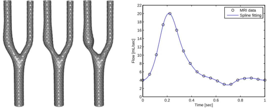
We have modeled a 10 cm long representative healthy carotid artery bifurcation
Figure 2. Top: two views of |u × ∇ × u|. Bottom: νnT(∇u)n on the wall of the vessel. The lower section of the tube faces the reader.
Figure 3. Computation of [~u, p] with (26) for an aorta. Left:
pressure at t = 0.8. The compliant walls are updated for graphic visualization of the compliant wall deformation. On the Left the
vertical velocity u3 at t = 0.8 without graphic enhancement, thus
carotid artery has a diameter of 9 mm, the internal and external carotid arteries have a diameter of 6.8 mm and 5.6 mm, respectively. All artificial boundaries are perpendicular to x- axis. Finite element meshes (coarse discretization h = 0.2 mm,
1885 vertices) are shown in Figure4. Fine discretizations are built with h = 0.04 mm
resulting roughly in 2 · 105vertices and one million tetrahedral elements.
First, in order to compare our results with those cited above, we consider Σ to be
a rigid wall. We also replaced the inlet boundary conditionR
ΓpΓuˆn by the velocity
profile
UΓ= 2 Q/ACCA(1 − y2/R2CCA− z
2/R2 CCA)
where Q is the flow rate depicted in Figure4(right). Spline interpolation was used
to fit the pointwise data; traction-free boundary conditions were imposed at the outlet boundaries.
The initial velocity-pressure field at t = 0 is set to be a solution of the Oseen equa-tion. The time step is 0.01. Five cardiac cycles are sufficient to eliminate transient effects caused by initial conditions, and to obtain cyclically repeated flow patterns.
For the considered geometries, the inlet flow together with ν = 3.5 ·10−3Pa·sec and
ρ = 1060 kg ·m−3 result in a Reynolds number of a few hundreds; Re at the inflow
surface is 357, Re at the 64% stenosed area is 1280. Excellent agreement with the published results was observed in booth magnitude and location of flow patterns.
0 0.2 0.4 0.6 0.8 1 0 2 4 6 8 10 12 14 16 18 20 22 Time [sec] Flow [mL/sec] MRI data Spline fitting
Figure 4. Carotid bifurcation: healthy (left), 30% (middle), 64% (right) stenosed models (coarse discretization). Flow rate waveform at the common carotid artery inlet.
Now we use model (26) with b = 200 and δt = 0.01. The geometry is fixed for the
numerical simulations but updated for graphic rendering, κ = 100. We observe that
for all three models the maximum positive displacement, i.e. expansion ( ~d · ~n > 0)
is at t = 0.17, while the maximum negative displacement i.e. contraction is at
t = 0.64. Figure 5 shows the updated shape of the bifurcation region at four
selected phases of the cardiac cycle: t = 0, t = 0.1, t = 0.15 and t = 0.17. The red color marks regions with higher pressure. We observe that the healthy artery undergoes a uniform expansion/contraction in the entire domain. For the stenosed arteries, displacements become much larger in the portion of the internal carotid artery below the bifurcation; we identify tiny displacements downstream from the stenosis. More importantly, a steep change in pressure near the stenosis region
observed for both 30% and 64% stenosis models will produce an increasing shear stress that could be a reason for arterial rupture.
t = 0.00 t = 0.10 t = 0.15 t = 0.17
Figure 5. Carotid bifurcation. Arterial displacement during the pre-systolic period; top to bottom: normal, 30%, 64% stenosis. Dark red color marks regions of higher pressure.
The present study has demonstrated that model (26) allows physiologically
realis-tic blood flow analysis. A hierarchy of approximations helps reducing the overall computational effort of updating the triangulation at every time step. On the other hand, the method allows to inspect arterial compliance at arbitrary phases of the cardiac cycle. More importantly, moving the geometry for graphic visualization can be done as a post-processing task, or in parallel.
REFERENCES
[1] C. Begue, C. Conca, F. Murat, and O. Pironneau. Les equations de Stokes et de Navier-Stokes avec condtions aux limites sur la pression, pp. 179-264. Pittman, RNM Longman, 1988. In H. Brezis, J. Lions (eds): Nonlinear Partial Differential Equations and their applications, College de France, Vol. IX. Pitman, Boston.
[2] D. Boffi, L. Gastaldi, A FEM for the immersed boundary method, Comput. Struct. 81(2003),491-501.
[3] M. Costabel and M. Dauge, Maxwell and Lam´e Eigenvalues on Polyhedral Domains. Preprint Universit´e de Rennes I, 2002.
[4] M. Costabel, M. Dauge. Singularities of electromagnetic fields in polyhedral domains. Preprint 97-19, Universit´e de Rennes 1 (1997). http://www.maths.univ-rennes1.fr/∼dauge/. [5] G.H. Cottet, E. Maitre and T. Milcent. Eulerian Formulation and Level Set Models For
Incompressible Fluid-Structure Interaction. ESAIM: M2AN 42 (2008) 471-492.
[6] P. Crosetto, S. Deparis, G. Fourestey, A. Quarteroni Parallel Algorithms For Fluid-Structure Interaction Problems In Haemodynamics. SIAM J. SCI. COMPUT. Vol. 33, No. 4, pp. 1598-1622 (2011).
[7] A. Decoene & B. Maury Moving Meshes with freefem++. J. Numer Math (20)3-4, p195-214(2013).
[8] J. De Hart, G. Peters, P. Schreurs and F. Baaijens. A three-dimensional computational analysis of fluid-structure interaction in the aortic valve. J. Biomechanics 2003; 36:103-112. [9] S. Deparis, M.A. Fernandez and L. Formaggia, Acceleration of a Fixed Point Algorithm
for Fluid-Structure Interaction using Transpiration Conditions. ESAIM:M2AN Vol.37,No 4,2003, 601-616.
[10] ˆA Fang Q. Hu, X.D. Li, D.K. Lin. Absorbing boundary conditions for nonlinear Euler and Navier-Stokes equations based on the perfectly matched layer technique. J. of Comp. Physics 227 (2008) 4398-4424.
[11] M. Fernandez, Incremental displacement-correction schemes for incompressible fluid-structure interaction. Numer. Math. (2013) 123:21-65.
[12] L. Formaggia, J.F. Gerbeau, F. Nobile, A. Quarteroni, On the coupling of 3D and 1D Navier-Stokes equations for flow problems in compliant vessels. Comput. Methods Appl. Mech.Engrg.191(2001)561-582.
[13] L. Formaggia, A. Quarteroni, A. Veneziani eds. Cardiovasuclar Mathematics. Springer MS&A series 2009.
[14] V. Girault, R. Glowinski, Error analysis of a fictitious domain method applied to a Dirich-let problem, Japan Journal of Ind. and Applied Math., 12, 3, 487-514 (1995).
[15] V.Girault,P.A.Raviart, Finite Element Method for Navier-Stokes Equations.SCM 5. Berlin, Heidelberg, NewYork: Springer 1986.
[16] ˆA O. Gonzalez, J.C. Simo On the Stability of Symplectic and Energy-Momentum Algorithms for Nonlinear Hamiltonian Systems with Symmetry. Comput. Methods Appl. Mech. Engrg. 134 (1996) 197-222.
[17] O. Gonzalez Exact energy and momentum conserving algorithms for general models in non-linear elasticity. Comput. Methods Appl. Mech. Engrg. 190 (2000) 1763-1783.
[18] K. Gostaf, O.Pironneau , and F.X. Roux. Finite Element Analysis of Multi - Component Assemblies: CAD - based Domain Decomposition. DDM 14 Proc. (to appear).
[19] I. Marshall. Computational Simulations and Experimental Studies of 3D Phase-Contrast Imaging of Fluid Flow in Carotid Bifurcation Geometries. Journal of Magnetic Resonance Imaging 31 (2010) 928-934.
[20] D.A. Steinman, T.L.Poepping, M. Tambasco, R.N. Rankin, and D.W. Holdsworth. Flow Patterns at the Stenosed Carotid Bifurcation: Effect of Concentric versus Eccentric Stenosis. Annals of Biomedical Engineering 28 (2000) 415-423.
[21] J. L. Guermond, P. Minev, and J. Shen. An overview of projection methods for incom-pressible flows. Comput. Methods Appl. Mech. Engrg., 195(44-47):6011-6045, 2006.
[22] M. Heil, A. Hazel, J. Boyle. Solvers for large-displacement fluid-structure interaction prob-lems: segregated versus monolithic approaches. Comput Mech (2008) 43:91-101.
[23] P. Le Tallec Fluid structure interaction with large structural displacements. Comput. Meth-ods Appl. Mech. Engrg 190, 3039-3067. 2001.
[24] F. Nobile and C. Vergana, an effective fluid-structure interaction formulation for vascular dynamics by generalized robin conditions. SIAM J. Sci. Comp. Vol. 30, No. 2, pp. 731-763 (2008).
[25] C. Pares Un traitement faible par ´el´ement finis de la condition de glissement sur une paroi pour les ´equations de Navier-Stokes. C. R. Acad. Sci. Paris S´er. I Math., Vol. 307, pp.101-106, 1988.
[26] C. Peskin, The immersed boundary method, Acta Numerica 11 (2002),479- 517.
[27] C. Peskin and D. McQueen, A three dimensional computational method for blood flow in the hearth-I. Immersed elastic fibers in a viscous incompressible fluid, J. Comput. Phys. 81 (1989) 372-405.
[29] O. Pironneau. Conditions aux limites sur la pression pour les ´equations de Stokes et de Navier-Stokes. C. R. Acad. Sci. Paris S´er. I Math., 303(9):403–406, 1986.
[30] OP and M.Tabata. Stability and convergence of a Galerkin-characteristics finite element scheme of lumped mass type Int. J. Numer. Meth. Fluids 2010; 64:1240-1253.
[31] R. Rannacher, Incompressible Viscous Flow. Encyclopedia Mecanicae. E. Stein ed. Wiley 2004.
[32] J. Rappaz, S. Flotron Numerical conservation schemes for convection-diffusion equations (to appear).
[33] Zhiyong Si. Second order modified method of characteristics mixed defect-correction finite element method for time dependent Navier-Stokes problems. Numer Algor (2012) 59:271-300. [34] J. Tambaca, S. Canic, M. Kosor, R.D. Fish, D. Paniagua. Mechanical Behavior of Fully Expanded Commercially Available Endovascular Coronary Stents. Tex Heart Inst J 2011;38(5):491-501).
[35] M. Thiriet, Biomathematical and Biomechanical Modeling of the Circulatory and Ventilatory Systems. Vol 2: Control of Cell Fate in the Circulatory and Ventilatory Systems. Springer Math& Biological Modeling 2011.
[36] F. Usabiaga, J. Bell, R. Buscalioni, A. Donev, T. Fai, B. Griffith, and C. Peskin. Staggered schemes for fluctuating hydrodynamics. Multiscale Model Sim. 10:1369-1408, 2012. [37] I. Vignon-Clementel , A. Figueroa, K. Jansen, C.A. Taylor Outflow boundary con-ditions for three-dimensional finite element modeling of blood flow and pressure in arteries. Comput. Methods Appl. Mech. Engrg. 195 (2006) 3776-3796.
![Figure 1. Top left: computation of [u, v, w, p, η] with (22). Top right: computation of [u, v, w, p] with (26)](https://thumb-eu.123doks.com/thumbv2/123doknet/12392633.331326/10.918.190.788.149.601/figure-left-computation-u-v-η-right-computation.webp)
![Figure 3. Computation of [~ u, p] with (26) for an aorta. Left:](https://thumb-eu.123doks.com/thumbv2/123doknet/12392633.331326/11.918.235.680.657.904/figure-computation-u-p-aorta-left.webp)